Multi-Level Energy Management for Hybrid Electric Vehicles—Part I


1
Department of Mechanical Engineering, Eindhoven University of Technology, 5600 MB Eindhoven, The Netherlands
2
DAF Trucks N.V., 5600 PT Eindhoven, The Netherlands
*
Author to whom correspondence should be addressed.
Vehicles 2019, 1(1), 3-40; https://doi.org/10.3390/vehicles1010002
Submission received: 2 October 2018
/
Revised: 15 January 2019
/
Accepted: 16 January 2019
/
Published: 15 February 2019
Abstract
:The fuel economy of a hybrid electric vehicle (HEV) is improved, by taking the energy relevant system states into account in the energy management system (EMS). With an increasing number of states and decision variables, energy optimizing algorithms in the EMS can be prohibitive for real-time implementation. In part I of this work, a model-based, multi-level approach is taken to subdivide the original (large) optimization problem into computational efficient sub-problems, based on optimal control techniques using a preview. The resulting EMS solves the problem of power-split between engine and motor/generator, mode and gear switching including switching costs, with battery energy constraints. The superior energy efficiency of the multi-level EMS is simulated on a representative heavy duty drive cycle, where it saves 7.0% fuel, compared to a conventional vehicle, where the baseline EMS for the HEV saves 5.8%. In part II, real-world validation of the EMS is performed.
1. Introduction
Hybrid electric vehicles (HEVs) have emerged as a promising solution to reduce operational cost in commercial road transportation, while complying to increasingly stringent emission legislation. Since HEVs have more than one power converter, they offer additional control freedom, compared to conventional vehicles, which give opportunities for the energy management system (EMS) to decrease fuel consumption and emissions. The EMS has to consider the energy relevant systems of the HEV and already a large amount of solutions have been proposed that take the battery energy dynamics into account [1]. However, the system efficiency can be further improved by taking additional system states into account as suggested by [2,3], referred to as a ‘unified’, ‘integrated’, ‘total’ or ‘holistic’ energy management. Examples of such additional systems are the battery with its temperature and aging characteristics [4,5], engine after-treatment system [3,6], waste-heat recovery system [7], combustion engine [8], or the cabin heater [9].
Using model information of these systems, the EMS can be posed as an optimization problem, in order to ensure energy efficiency. The computational complexity of this problem, however, increases with the number of states, presence of state constraints, number of decision variables, type of decision variables (continuous/discrete) and nonlinearity of the models. Many methods exist to design an optimizing EMS, using e.g., Dynamic Programming [10,11], Pontryagin’s Minimum Principle [12] or Model Predictive Control [13,14] and generate close to optimal results; however they can be computationally too demanding for real-time implementation. In this work, a combination of methods is used, to ensure an efficient computation for each of the sub-problems.
An overview of real-time implementable optimization approaches for a (parallel) hybrid vehicle with the decision variables: power-split, stop-start and gear selection, is given in Table 1. In particular, discrete control variables increase the computational complexity, explaining why gear selection is often omitted from the EMS or solved in a separate step with heuristics [15,16,17]. In [18], an integrated approach is presented, where gear selection and stop-start are part of a sequential optimization with the power split. In these approaches, the cost of stop-start and gear change events are not considered, which can result in unacceptable switching behaviour, like hunting oscillations. To overcome this problem, costs on switchings are included, solved using Dynamic Programming (DP) and Quadratic Programming (QP) [19] or as one Mixed Integer Linear Program (MILP) [20]. For real-time solving, the allowed model complexity is limiting and adding additional states to these EMSs is computationally prohibitive.
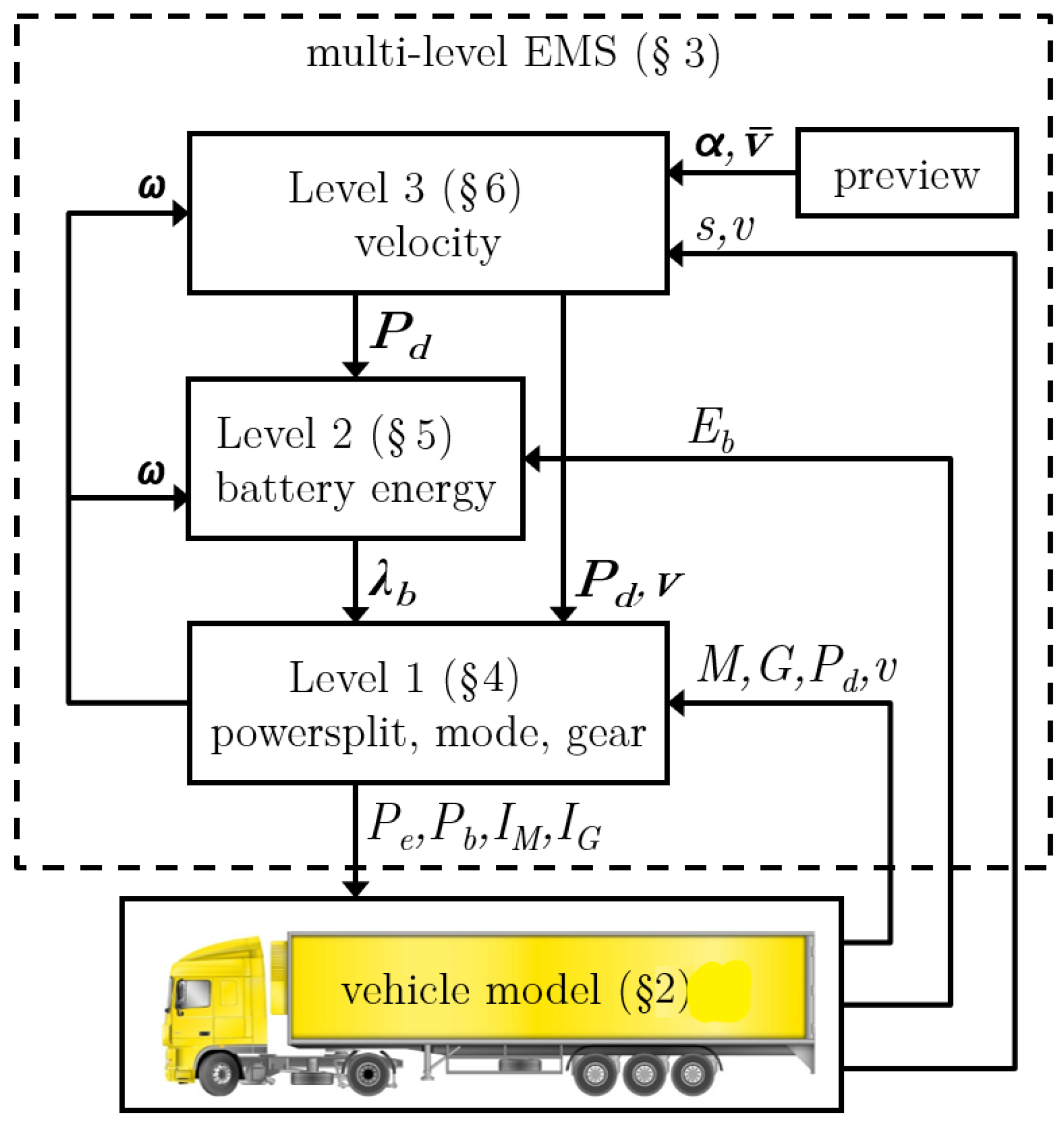
By partitioning a large optimization problem into a set of smaller problems, as in a distributed control system [21], the computational efficiency and robustness are improved, albeit losing the guarantee of global optimality. The process of partitioning is not trivial and many different structures exist. For the power-split problem, two-level structures can be identified in literature [22,23,24], where planning of the battery energy is separated from the power-split decisions. In this work, a novel EMS is developed as a multi-level system [25,26], in which the higher layers have an increasing level of abstraction of the system, to be able to optimize and coordinate the lower layers [27], while having a large decoupling between the levels. The multi-level EMS solves this control problem with preview, for real-time implementation, using optimal control techniques (PMP and DP), thereby eliminating calibration of parameters. In Figure 1, the proposed control system is illustrated. Each level minimizes fuel, however, dependent on the function of the level, different model information and corresponding optimal control techniques are used.
- On the first level, the power-split is explicitly solved using the Pontryagin Minimum Principle (PMP), starting from [15]. This method is extended with costs on mode and gear switching, thereby eliminating unacceptable switching behaviour. A Dynamic Programming (DP) routine solves the discrete subproblem. Route and vehicle information determine the switching costs, supporting a full model based approach.
- The second level optimizes the battery state of charge with input- and state-constraints, and provides efficiency information of the hybrid system to the other levels using the battery costate from the PMP solution. Due to the mode switching system on the vehicle, charge sustaining behaviour must be enforced, by using an additional switching algorithm between non-unique solutions.
- The third level provides the necessary route information to the lower layers. By predicting the velocity along the route, using road slope and velocity limitations, the road load on the driveline is determined.
In Section 2, the model of the parallel hybrid vehicle is described, after which the multi-level EMS for this vehicle is formulated in Section 3. The algorithms used on each of the three levels are explained in Section 4 (power-split, mode and gear switch optimization), Section 5 (battery energy optimization) and Section 6 (velocity prediction). Offline and online solution schemes of the multi-level optimization are compared in Section 7, where high fidelity simulation results show the fuel benefit of the algorithm. The conclusions are drawn in Section 8. The real-world validation of the multi-level EMS is described in [28].
2. Parallel Hybrid Electric Vehicle Model
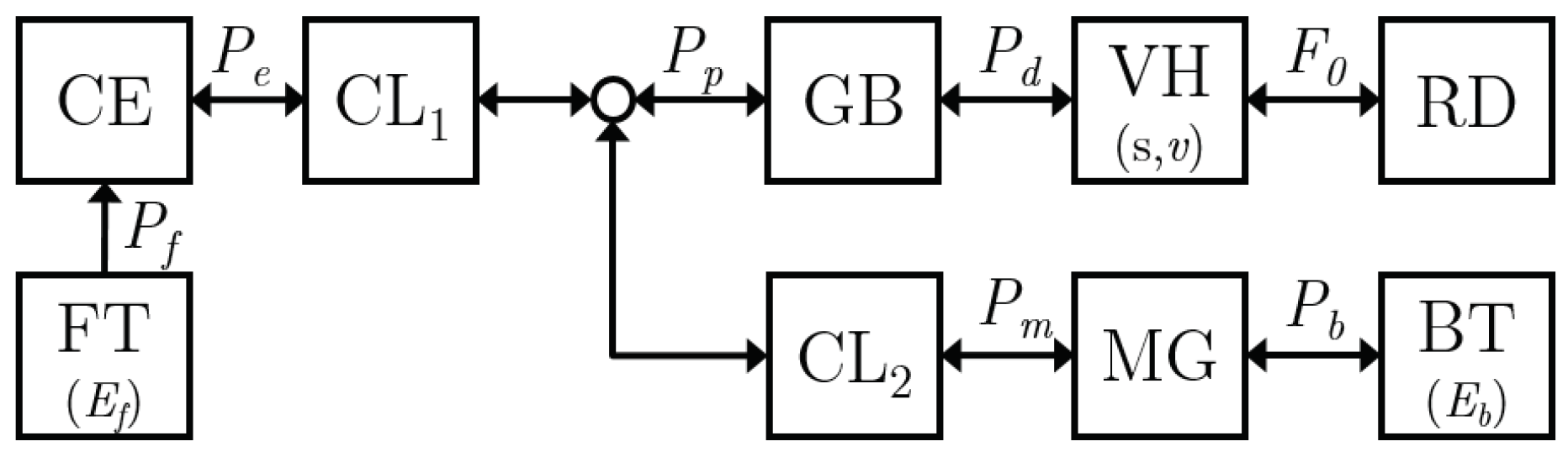
For the design of a model-based EMS, the applied models of the hybrid electric vehicle (HEV) are described in this section. The parallel hybrid vehicle under consideration is schematically depicted in Figure 2. The fuel power flows from the tank (FT) to the Combustion Engine (CE), converted to mechanical power , thereby depleting the available fuel energy . Dependent on the position of the clutches CL and CL, the power from the Motor/Generator (MG) is added to , resulting in the power at the power-split point . This power is transferred through the gearbox, final drive and wheels (GB), resulting in the driveline power of the vehicle (VH). Dependent on the road load acting on the vehicle (), the travelled distance s and velocity v will change. The MG exchanges electrical power with the battery (BT), thereby (dis-) charging the buffer . Due to the two clutches, both CE and MG can be disconnected and stopped, thereby eliminating their friction losses. In the following sections, the models for this topology are given, with typical model parameters denoted in Table 3.
2.1. Internal Combustion Engine
The internal combustion engine (CE, or ‘engine’) is modeled as an affine relation between the fuel and the power output , often referred to as a Willans approximation [29]:
with the indicated efficiency (see Table 3) and the speed dependent friction losses. It should be noted that and . The power output is limited by
as shown in Figure 3. The CE has , meaning that additional engine braking can be applied on top of the nominal friction, which is a feature typically available on heavy duty commercial vehicles. For , no fuel is consumed (). The total fuel consumption is the integral of :
2.2. Motor Generator
2.3. Battery
The battery (BT) is modeled as an integrator, with quadratic losses, see [15]:
with the energy in the battery, the internal battery power, the power at the terminals and the loss constant. Note that discharges the battery. The effective size of the battery is limited, such that
In [8], the validation of the compression-ignition engine (CE), motor generator (MG) and the battery (BT) model is described.
2.4. Mode Selection
The topology has two clutches, CL for connecting the CE to the driveline and CL for connecting the MG to the driveline. When the clutch is open, the respective component is disconnected from the driveline and stopped to eliminate the friction losses in the component. The two clutches create four modes , representing the driveline states, as defined in Table 4. If connected, then the rotational speed of the CE(), respectively, the MG (), is equal to the rotational speed at the gearbox input shaft, and zero otherwise. The gearbox input power is the sum of the connected components.
The mode is controlled with for the respective four modes. Mode switch dynamics are defined by the state machine in Figure 4. When a mode switch () is performed, the driveline is open () for a duration of , during which no traction is available (). During the mode switch, a series of events, involving (de-)coupling and synchronization of rotating masses, cause energy losses, represented by the lumped parameter :
In Appendix C, the dependency of on the driveline state and the drive cycle is described.
2.5. Gear Selection
The gearbox with final drive and wheels (GB) is modeled as a geometrically stepped transmission without losses. The ratio of the gearbox is a function of the gear position with the gear base constant
The gearbox input shaft speed [rpm] is related to the vehicle speed v [m/s], through the gearbox ratio, final drive and wheels, with
where is the drive ratio from speed [m/s] to gearbox out [rpm]. The gear selection is controlled with . Gear switch dynamics are defined by the state machine in Figure 5. When a gear switch () is performed, the driveline is open () for a duration of , during which no traction is available:
During the gear switch, a series of events, involving (de-)coupling and synchronization of rotating masses, cause energy losses, represented by the lumped parameter :
In Appendix C, the dependency of on the driveline state and the drive cycle is described.
2.6. Vehicle
The dynamics of the vehicle (VH) are modeled for the longitudinal motion:
with vehicle mass m, vehicle position s, the vehicle speed, and the total vehicle road load :
with:
respectively, the air drag, rolling resistance and gravitational force, and the driveline force:
where is the road inclination, and the other parameters as defined in Table 3. The velocity of the vehicle is limited, such that
with the maximum speed limit.
3. Multi-Level Energy Management
Optimizing the energy consumption for a system, with multiple states and a mix of continuous and discrete decision variables, is computationally demanding for real-time implementation. Partitioning the optimization into smaller problems reduces the computational burden. Not only are the sub-problems smaller and thereby easier to solve, but also each partition can have its own optimization algorithm, making the selection of more efficient algorithms possible, suited to the specific problem of that partition. e.g., in [19] Dynamic Programming is used for the partition with discrete decision variables, while convex optimization is used for the partition with continuous states. The method of partitioning is, however, not unique nor trivial [27].
For the generic energy management problem, described in Section 3.1, a functional hierarchy is introduced in Section 3.2, inspired by the ‘multi-level structure using conjugate variables’ in [27]. In this section, the partitioning in levels, and the solution of the multi-level EMS, for two solution schemes, are described:
- the iterative scheme (Section 3.3), used in simulation to show convergence of the EMS in Section 7.1,
- the model predictive scheme (Section 3.4), that is real-time implementable and simulated in Section 7.2.
3.1. Generic Energy Management Problem
The general task of the Energy Management System (EMS) is to minimize the fuel energy needed to move the vehicle from distance to . For the vehicle model in Section 2, this EMS can be posed as a nonlinear, mixed-integer, input- and state-constrained dynamical optimization problem:
with continuous decision variables (driveline power), (battery power) and discrete decision variables (mode request), (gear request):
continuous states s (distance), v (velocity), (battery energy) and discrete states (mode), (gear):
disturbances, representing the preview information, (road slope), (maximum velocity):
switching cost (for mode switch), (for gear switch):
equality constraints on (initial distance), (final distance), (battery energy) sustenance:
inequality constraints on v, upper and lower limits, (CE power) upper and lower limits, (MG power) upper and lower limits:
together with the model equations in Section 2.
3.2. Multi-Level Optimization
In the multi-level EMS, the global optimization problem is subdivided into three levels based on its function: velocity determination, optimizing battery energy and optimizing the power-split including switching of modes and gears. Each level (indicated with subscript ) has the same objective, i.e., minimizing (equivalent) fuel:
but with a subset of the decision variables, and on each level a different model complexity, belonging to the abstraction and dynamics on that level. In Table 5, the sub-problems of the optimization are defined, including the output y of each level. Numbering of the levels start at 1 for the lowest level, as control of the component itself (e.g., for safe operation) is indicated with Level 0, and is not contained in the EMS. Information exchange between the three levels is shown in Figure 1 and the function and interfacing of each level is briefly explained next.
3.2.1. Level 1, ‘Power-Split Including Switching’ (Section 4)
Level 1 is the lowest control level in the EMS, responsible for the optimal power split (defined by and given ), mode () and gear () selection. Based on information from the higher levels, it has to act fast, in order to have a responsive vehicle. However, the required fast update rate (typically 10–100 Hz) limits the computational time available for calculations. This is solved by moving computational expensive calculations to higher layers, and having explicit solutions for the remaining optimizations, using optimal control techniques (DP and PMP, see Appendix A). Information from the higher levels is provided by vectors over time (indicated in bold) with estimated quantities:
- , estimated equivalent cost of battery energy,
- , estimated power demand,
- , estimated vehicle speed,
and, after optimizing the decision variables, the calculated driveline speed is provided to Levels 2 and 3.
3.2.2. Level 2, ‘Battery Energy’ (Section 5)
Level 2 is responsible for optimizing the battery energy over the cycle, considering the battery constraints. As the battery energy dynamics are slower than the decisions needed in Level 1, its optimizations can run at a lower rate (typically 1 Hz), facilitating the more complex calculations, caused by battery limits and longer horizons. Abstraction of the Level 1 model, by e.g., not considering gear switching and no penalties on switching, combined with PMP techniques, make the optimization computationally efficient. Based on an estimated driveline speed , the estimated power demand and the current battery energy , the optimal is calculated, which is input for Level 1.
3.2.3. Level 3, ‘Velocity’ (Section 6)
Level 3 determines the velocity . Of the three levels, it uses the most abstracted model of the hybrid driveline, by e.g., not considering battery dynamics, hybrid modes, power-split or switching. Using-distance based route information for preview, i.e., slope and maximum speed limits , and current vehicle velocity v and position s, an estimate speed is determined, resulting in an estimated power demand .
3.3. Multi-Level Iteration
The multilevel iteration scheme is used for offline simulation. In this multilevel, nested, optimization, the decisions on one level impact the objective on other levels and thereby influencing optimality [21,30]. This dependency can be seen in Figure 1, where the variables and , are fed back to the higher level controllers. Solving the optimization by starting at the highest level and sequentially transmitting information to the lower levels, we need an a priori estimate of and . When all levels are calculated, the sequence can be repeated, where and are updated from the last sequence, thereby providing the higher levels with the latest decision details of the lower levels. The solution scheme of the optimization results in:
- Initialization:
- (a)
- all levels optimize over the complete drive cycle, from to final time ,
- (b)
- initialize with an estimated average speed,
- Velocity prediction:
- (a)
- retrieve , (road slope and speed limit information), , (position and speed) and model parameters (Table 3),
- (b)
- use the vehicle model and results from optimal control, to predict the velocity profile,
- (c)
- store resulting , .
- Battery energy optimization:
- (a)
- retrieve , , and model parameters (Table 3),
- (b)
- calculate PMP necessary conditions and optimize the remaining boundary value problem(s),
- (c)
- store resulting .
- Power-split and switch optimization:
- (a)
- retrieve , , and model parameters (Table 3),
- (b)
- calculate PMP necessary conditions and solve the remaining DP problem,
- (c)
- store resulting and output , , , to the component controllers on the vehicle.
- Iterate:
- (a)
- repeat from step 2 with an improved estimate of and , unless stop conditions are met (number of iterations). Note that the initial conditions at remain identical.
It is expected that each iteration will increase fuel efficiency, until the solution is converged. The effect of the number of iterations on the fuel efficiency, is analyzed by simulation in Section 7.
3.4. Multi-Level Model Predictive Control
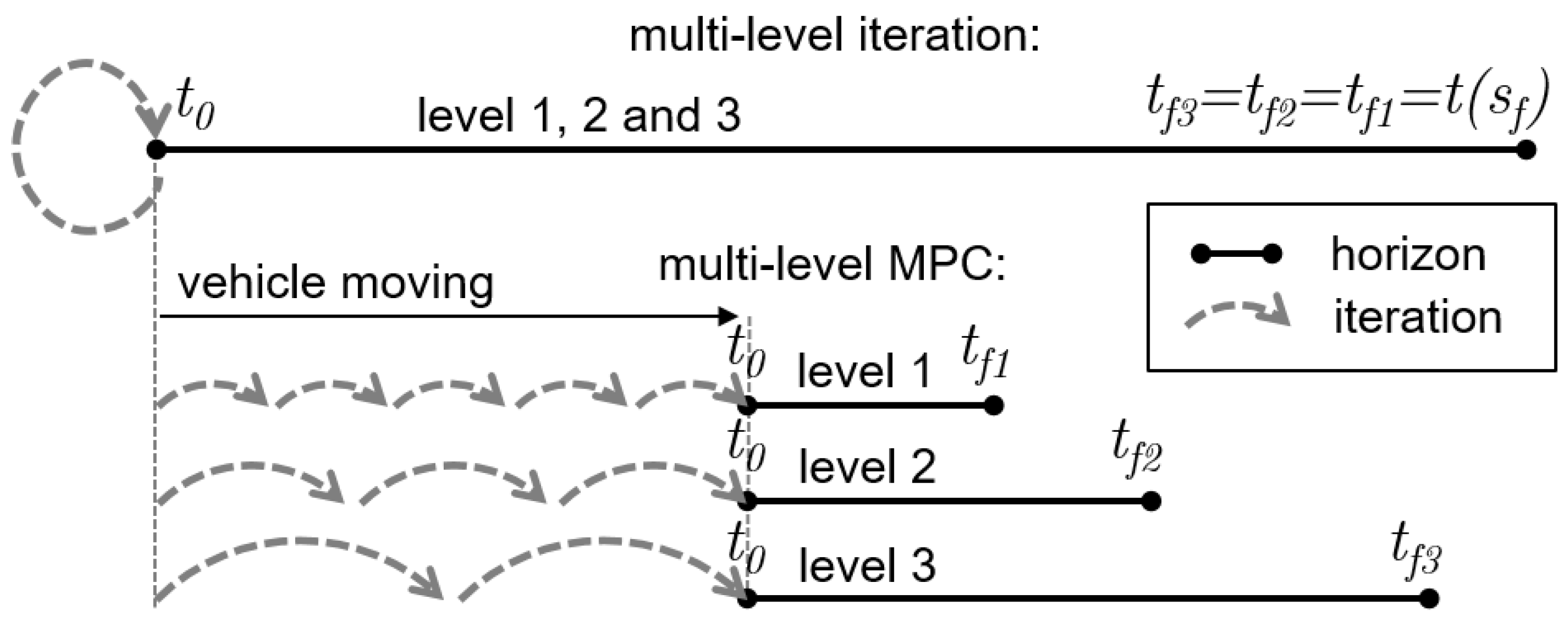
To apply the EMS in real time, the multilevel optimization is implemented as a model predictive (or receding horizon) controller (MPC), which performs the optimization in a regular schedule (‘sampling’). Each sampling period the optimization is performed with updated states, over a subset of the cycle (‘horizon’), thereby creating feedback for disturbance rejection and model mismatch compensation. In Figure 6, the differences with the multi-level iteration, in horizon and iteration, are illustrated. Compared to the solution scheme in Section 3.3, the following adjustments are made:
- now refers to the vehicle’s current time and is relative to , with a fixed horizon length (which implements the receding horizon),
- each sample time, only one iteration is applied, i.e., step 5 in the iteration scheme is skipped,
- the horizon length decreases on each level: ,
- each level runs in its own regular schedule (sample time), where the higher levels run slower than the lower levels.
All adjustments are for improving computational efficiency; however, optimality will reduce. In Section 7, we will show that, in simulation, the optimality is marginally decreased and the multi-level approach shows good fuel economy in a high fidelity simulation environment. In Section 4, Section 5 and Section 6, the algorithms are described in detail for Levels 1, 2 and 3, respectively.
4. Level 1: Power-Split and Switch Optimization
The Level 1 optimization calculates the optimal power-split, mode and gear selection for a simplified plant model, as a subset from optimization (21). In [8,15], it is shown that the power-split problem with battery dynamics can be efficiently solved using PMP, resulting in two solutions steps, see Appendix A:
- minimization of the Hamiltonian as a function of , resulting in the optimal power-split, mode and gear,
- calculation of that complies to the battery constraints.
Level 1 performs the first step: minimization of the Hamiltonian. The second step, calculation of , is performed at Level 2, as described in Section 5.
On Level 1, we assume a predetermined velocity profile , which defines using in Equations (14)–(19). As is controlling (see Section 5), all continuous states () are removed from Equation (23), together with the equality and inequality constraints on the respective states in Equation (26) and Equation (27). As a result, the minimization Equation (28) for Level 1, denoted with subscript , is
with
with the switching cost in Section 4.1 and Section 4.2 and with in Section 4.3.
4.1. Explicit Minimization of the Hamiltonian per Mode
On Level 1, the Hamiltonian is minimized. For the hybrid drive train, this Hamiltonian is solved explicitly in [8,15], i.e., an analytical expression is found for the minimization. This section extends that solution for the driveline topology with an additional clutch between MG and GB. The Hamiltonian of Level 1 to minimize is
using the PMP conditions (Appendix A). When we assume instantaneous switching, i.e., , the control signals and bring the system immediately to its corresponding state, hybrid mode M, respectively, gear G, such that . Then, for each , the minimum of is found by solving . For each , the result is given in Table 6, where only parameter depends on the rotational speed , as defined by G and v through Equation (11).
With the explicit expression for (where the superscript denotes the optimal solution), the reduced Hamiltonian (with subscript denoting the variant) is an explicit expression, for each mode and gear combination. Finding the optimal is thereby reduced to:
In Figure 7, is illustrated. As a function of , changes modes at and . Due to the mode changes, the control signal for jumps as a function of at and , as shown in Figure 8. That jumping behaviour, caused by the additional clutch between MG and GB, is new to [8,15] and adds complications to the controllability of , as will be shown in Section 5.2.
4.2. Mode Selection, without Cost on Switching
Instead of calculating all and selecting the minimal one in Equation (36), a computationally more efficient approach can be taken where the optimal mode is calculated beforehand. Figure 7 shows that the optimal mode is changed at , and where the Hamiltonians of two modes are equal. Equating the Hamiltonians, using Equations (1), (4), (7), (36) and Table 6, results in five expressions, representing all the switching lines (guards B) where the optimal mode is changing. Two guards are a function of :
and three guards are a function of ():
All optimal modes are explicitly defined with Equations (37)–(41), as a function of () and the model parameters (Table 3). In Figure 9, the guards and optimal modes are illustrated.
A further reduced Hamiltonian is now obtained in three steps:
- for each (feasible) gear, calculate ,
- select that minimizes ,
thereby reducing Equation (36) to:
which statically defines the decision variables as a function of .
4.3. Mode Selection, with Cost on Switching
When the system operates near the guards, frequent switching (so called ‘hunting’) between modes and gears can occur under influence of disturbances, thus preventing acceptable real-life implementation. Each switch involves connecting and/or disconnecting of components, synchronization of their speeds and additional friction losses, which cause driveability, durability and efficiency issues. As a solution to hunting, the cost function in Equation 21 adds a penalty on mode switching and gear switching .
The parameters can be tuned to balance hunting behavior, with fuel economy. To prevent tuning of the parameters, Appendix C quantifies the model-based, equivalent fuel losses during a switch, identified by:
- synchronization losses, caused by acceleration and deceleration of rotating masses (Appendix C.1),
- traction interruption, caused by disconnection of the driveline and leading to vehicle speed deviations (Appendix C.2). As the speed deviation during disconnection of the driveline, depends on the road load (e.g., up-hill resulting in a large speed decrease, on flat road resulting in a small speed decrease), the corresponding equivalent fuel costs are a function of the speed change and time loss.
The calculated penalties are then a function of mode change, gear change and vehicle speed. Adding the cost of switching, changes Equation (29) to the new Level 1 cost function
which is the integral of the explicit Hamiltonian solution in Equation (36), with switching costs and added to the integral, when a switch occurs. By discretizing time,
with the discrete time vector and sampling time , the optimization is solved using Dynamic Programming. The outline of the algorithm is as follows, as illustrated in Figure 10:
- all feasible modes M and gears G over the time horizon are enumerated,
- for each combination of mode and gear and time, the Hamiltonian is explicitly solved using Equation (36), resulting in
- a Dynamic Program (DP) is formulated with as elements for the cost-to-go matrix
- to implement the cost for switching, for each mode change and gear change, the cost-to-go matrix is penalized with and ,
- the optimal sequence of modes and gears is calculated using DP,
- for the MPC implementation, only the first control action is implemented. The next sample time, the algorithm is repeated with updated inputs, disturbances and states.
5. Level 2: Battery Energy Optimization
The Level 2 optimization determines , which is an input for Level 1 control. That is found by solving the power-split problem, taking the battery dynamics in Equation (23), with corresponding limits (, , in Equation (27) ), into account.
On Level 2, we assume:
- a prescribed rotational speed , which defines with the predetermined velocity profile. Before iteration over the levels an estimated average is selected. After each iteration, from Level 1 is used.
- mode and gear switching is instantaneous (), without costs associated ().
Following [31], this dynamic state constrained problem is solved using PMP (Appendix A). Using Equations (6) and (7), the system dynamics are:
and with Equation (3) result in the Hamiltonian:
where is the costate of . As no switching costs are defined, is explicitly minimized with Equation (42) as a function of , among others. The dynamics of in Equation (A6),
show that is constant for the problem without constraint in Equation (8), or changes stepwise where is constrained [8,32]. Solving the problem is reduced to a boundary value problem [1], with the decision variable. The boundary value problem, for the topology with clutches, state constraints and a limited horizon, has the following properties, which are handled by the developed algorithms in this section, with the flowchart in Figure 11:
- I1
- Constraint activation increases the number of boundary value problems to solve, where the number of sub-problems is not known a priori. The iterative solution method from [32] is recapitulated in Section 5.1.
- I2
- Controllability of is not a continuous function of , due to the clutches in the topology, resulting in non-unique solutions. The switching algorithm in Section 5.2 ensures controllability for all .
- I3
- When the horizon does not include , the end condition on is not known, thereby removing charge sustenance as a control target. In Section 5.3, a solution is proposed, which is guaranteed to be optimal for a subset of scenarios.
In the remainder of this section, for ease of notation, but without loss of validity of the Level 2 problem where .
5.1. Constraint Handling (I1)
The optimal solution to Equations (21)–(27) results in a constant when constraints are not present in Equation (54), which can be efficiently found by solving the two-point boundary value problem. When constraints on are violated, the original problem must be subdivided into one or more subproblems dependent on the amount of constraint violations, as described in [32]. As we elaborate on this procedure in the next sections, we repeat an outline of the procedure here:
- The unconstrained subproblem is solved for a constant .
- If no constraint violation is present, the subproblem is solved. The procedure is repeated for the next unsolved subproblem.
- If constraint violations are present, the time of the largest constraint violation is identified. The subproblem is divided at into two new subproblems, with the first subproblem, having as an end point constraint and the second subproblem having as a start point constraint, when is violated. For violations .
This sequence is repeated, until all subproblems are solved, resulting in a piecewise constant for the whole cycle.
5.2. Controllability of : Non-Uniqueness (I2)
The optimal solution has a non-continuous controllability as a function of , leading to problems in realizing charge sustenance. The cause are the guards in the optimal solution of H (see Section 4.2), where a switch from one mode to another is enforced. When and coincide with one of the guards B, the optimal solution is non-unique (singular), i.e., several control inputs lead to the same fuel optimum [31,33,34].
The first type of guards are a function of (and ), i.e., , , (see Section 4). As normally varies in time, the optimal solution will seldom be at one of the guards for a prolonged duration. For that reason, Ref. [15] selects one mode a priori, when is on the guard, thereby being optimal, but without a guarantee to be charge sustaining. In simulations, especially with perfectly constant , switching between the modes could be necessary for a charge sustaining solution. Therefore, Ref. [18] opts to vary around , which causes switching between the modes, but is inherently sub-optimal because of the deviation from . In [33], this is correctly solved by using a so-called ‘sliding mode’ control, which minimizes the number of mode changes, which does not change . In our EMS, we also unalter and remain in the last mode, when coincides with the guards , , .
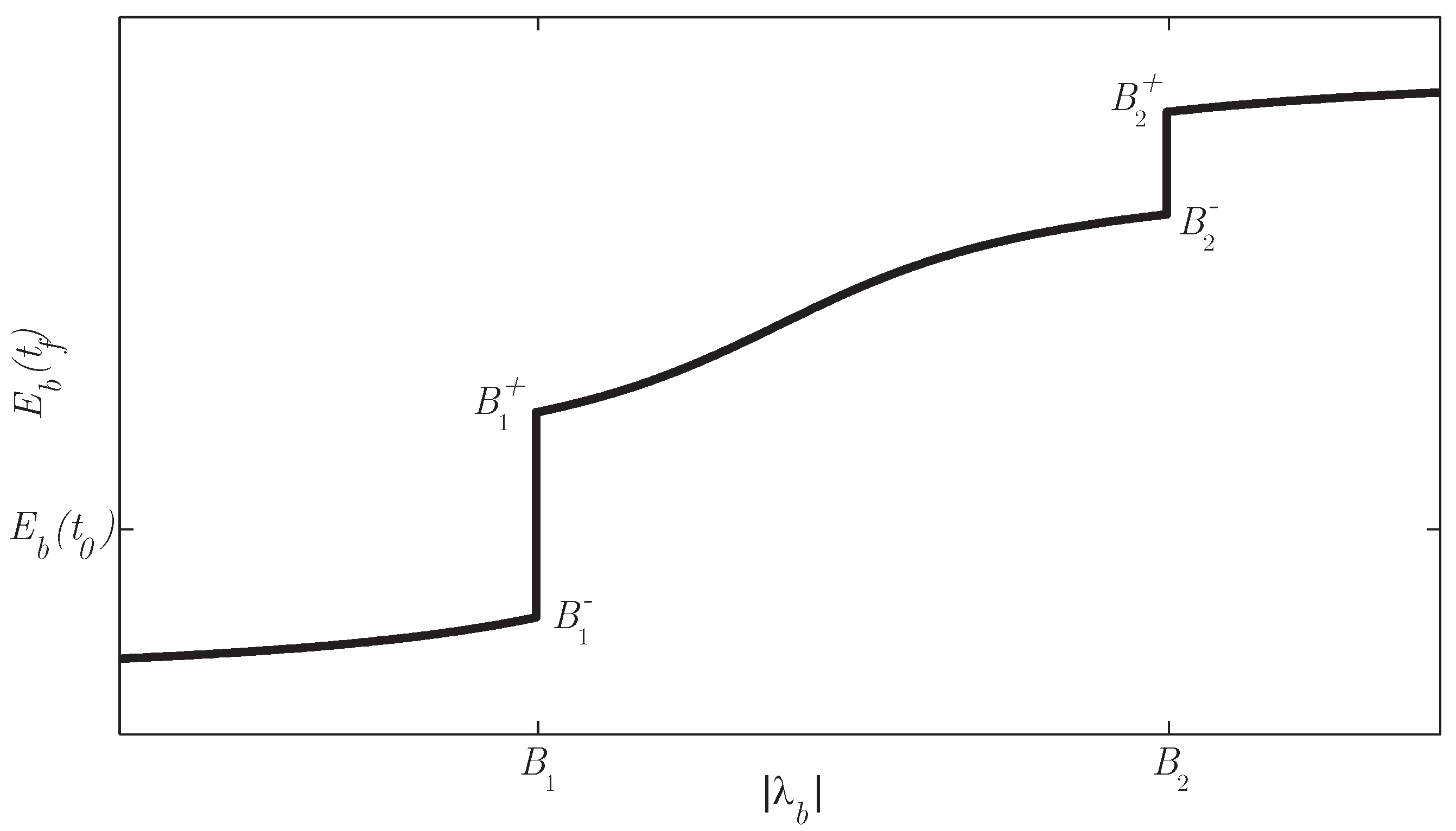
The second type of guards is not a function of , only of , i.e., and . As is (piecewise) constant, the solution can be on and for a prolonged period of time. Figure 8 shows that the optimal solution switches from to when is at guards or . Consequently jumps at and , and, for an arbitrary drive cycle, the controllability of (or charge sustenance) jumps as a function of —see Figure 12.
To have continuous controllability of in and , a switching sequence must be chosen and, in the following sections, algorithms for the two (extreme) switching scenarios are explained:
- I2a
- with an infinite number of switchings,
- I2b
- with a minimal number of switchings (elaborating on [33]).
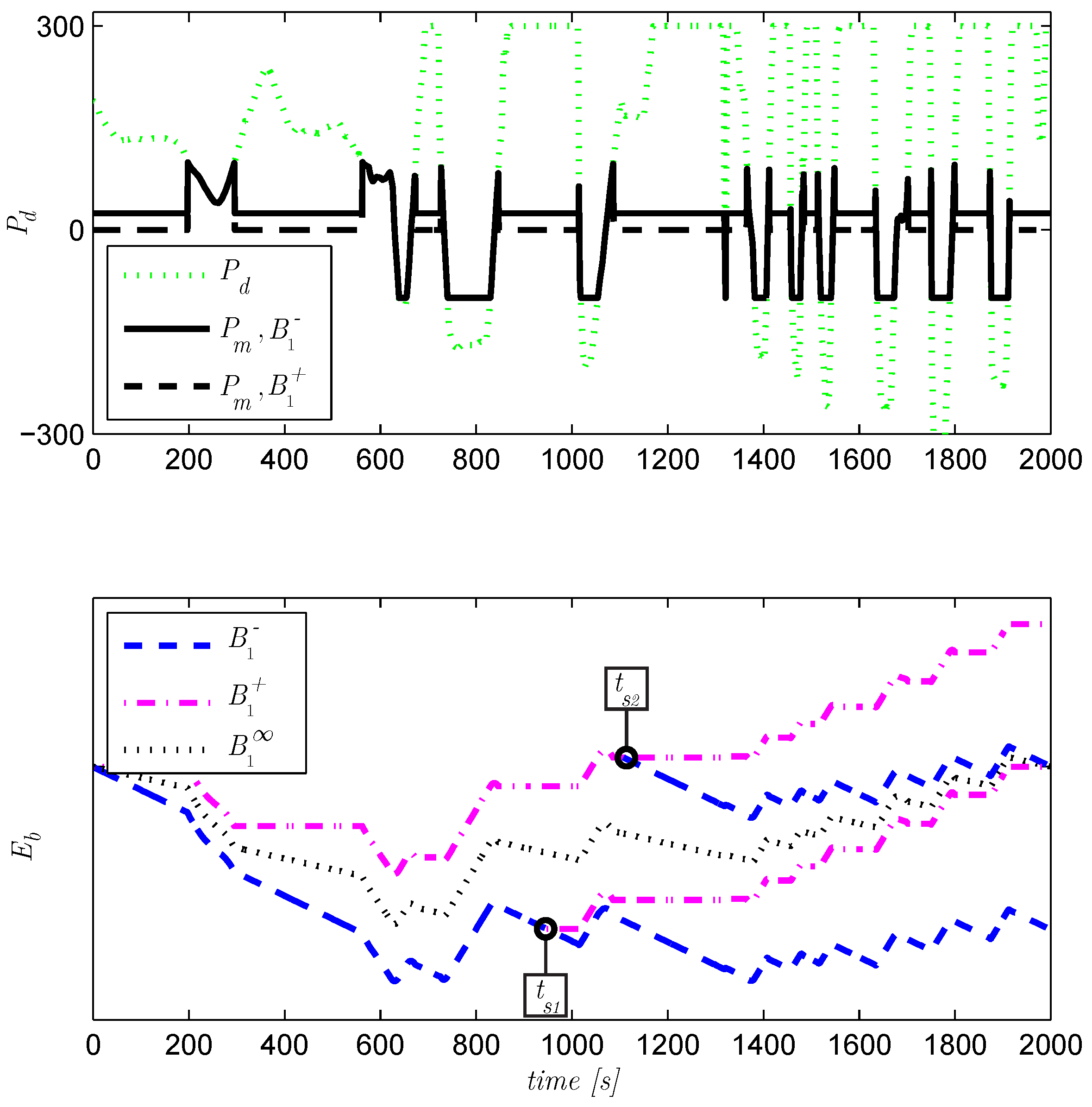
The switching scenarios are illustrated for a drive cycle of 2000 s, see Figure 13, for which coincides with . Trajectory (dash-dotted line) starts at and is above charge sustaining at s. Trajectory (dashed line) starts at and is below charge sustaining at s. In the top plot, is shown for both trajectories, where the difference is in supporting the CE with MG or not (boosting). The charge sustaining solution consists of switching between and over time, such that . At least one switch must be made, i.e., at or dependent on the initial mode. The next subsections provide algorithms to determine the switching sequence, taking constraints on into account. The algorithms, as illustrated for , also hold for .
5.2.1. Infinite Number of Switchings (I2a)
As the dynamics of in Equation (6) are state independent, a charge sustaining solution can be realized by taking a linear combination of the two trajectories and , such that:
where r is a ratio between 0 and 1. In the example in Figure 13, this combined solution is charge sustaining with (dotted line). This combined solution implies an infinite amount of switchings between the two trajectories, and will be referred to as .
5.2.2. Minimal Switching (I2b)
To enforce minimal switching, considering constraints on , a combination of algorithms I1 and I2a is needed. First, it is checked if the subproblem must be further subdivided as in Section 5.1 to guarantee within its bounds:
- if , then procedure I1 for constraint handling is performed,
- if , then procedure I1 for constraint handling is performed,
- if exceeds limits, then procedure I1 for constraint handling is performed,
- else a switching sequence exists in order to maintain within bounds.
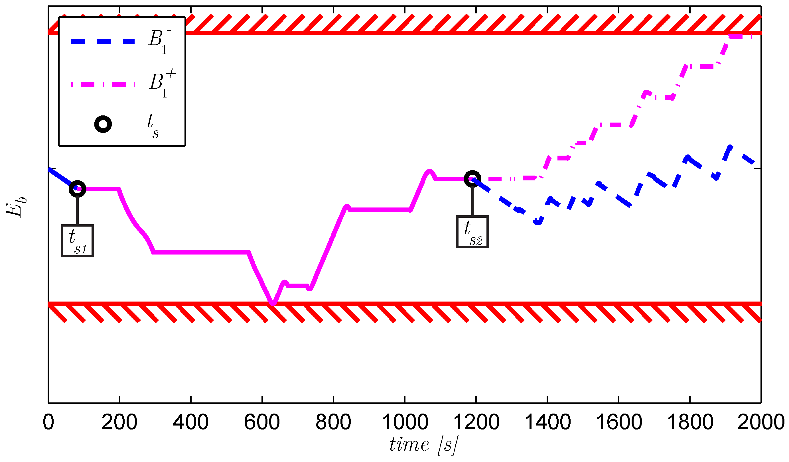
The switching sequence with minimal switchings is determined, by choosing when to switch between the two state trajectories and . The algorithm is illustrated in Figure 14 and Figure 15.
- The initial mode M is maintained, here resulting in
- Check for constraint violations. violation is detected at s, so switching to is mandatory. Switching at s results in undershoot of . With the known relative trajectories of and , the advancement of the switching time is determined, here at 83 s, Figure 15,
- The previous step is repeated, until is reached,
- is now within limits, but not at . A switch to the other mode is back propagated from , resulting in a last switch at 1191 s.
With this procedure, the discontinuity in the controllability of is solved with a switching sequence between modes, where the number of switchings is minimal. The value of has not been altered.
Note that knowing the switching sequence is not necessary on Level 2, as the interface from Level 2 to Level 1 does not use , but , which is not influenced by the switching sequence. Knowing that a switching sequence exists is thereby sufficient. The Level 1 optimization then decides on switching, taking switching costs into account (Section 4.3).
5.3. Limited Horizon (I3)
When is prescribed, the boundary value problem is fully defined and the optimal solution can be found. However, in real life, is only prescribed if the complete drive cycle is used (full horizon) and has a value, e.g.,
- for a repeating cycle, with , which is often used in simulation assessments,
- when entering a zero-emission zone at , with for maximal electrical driving after ,
- when arriving at a charging station at , with for cheap charging of the battery after .
If the prediction does not include , e.g., when implemented as a receding horizon algorithm, is undefined.
The following, suboptimal, procedure aims at finding a constant , without constraint violations, resulting in a trajectory that has maximal robustness towards constraint violations. Here, it is chosen to maximize the minimal distance of the trajectory to the constraints, in order to allow for disturbances in the prediction, without violating constraints. The outline of the procedure is:
- choose based on bi-section and simulate ,
- find the time index of and ,
- calculate the distance to the boundary for the two indices and select the minimal distance,
- select the next with bi-section, to increasing the minimal distance, and iterate.
The iteration stops when the increment of the minimal distance is smaller than a tolerance value. When the resulting violates constraints, the problem is subdivided as described in Section 5.2 and each sub-problem is evaluated again.
For two special cases, the above procedure results in optimal solutions:
- I3a
- if within the horizon, a limit is activated, irrespective of the control action e.g., due to a large energy recuperation event, the first subproblem up to this event is fully defined. The solution to this first subproblem is then optimal, and independent from the following subproblems.
- I3b
- if is on guard resulting in non-unique solutions and the non-unique solutions are able to span , is optimal for all .
With these algorithms, the calculation of the output of Level 2 () is complete.
6. Level 3: Velocity Prediction
The Level 3 functionality determines the velocity profile of the vehicle, given the slope and velocity limitations of the drive cycle, and provides the Level 2 and Level 1 algorithms with an estimated power demand and velocity . This section describes a simplified solution using results from the optimal control formulation.
Velocity Prediction Using Three Driving Modes
The Level 3 functionality predicts from information of the road ahead, i.e., road slope and velocity limitations . The velocity of the vehicle determines the resulting road load, so assumptions have to be made how the vehicle will accelerate/decelerate over the route. To determine the fuel optimal velocity profile, an optimization has to be solved. In [35], this optimization is performed for a conventional driveline with an affine fuel map, resulting in a set of three possible driving modes:
- maximum acceleration with ,
- minimum acceleration with ,
- constant speed , with .
The acceleration limits depend on the capabilities of the drive-line force , for a given road load . When we assume a continuously variable gearbox ratio, controlled to a fixed engine speed, and only one hybrid mode , Equations (2), (11), (15)–(19) and Table 4, define the acceleration limits as a function of velocity and road slope: and . For simulation, the vehicle model is completed with Equation (14). We use the three modes, to predict the velocity profile, given the road information and the vehicle model. The outline of the algorithm is given:
- retrieve and from the preview data source, for the drive cycle,
- decide on , typically the reference speed of the speed control on the vehicle,
- simulate the vehicle model forwards over the drive cycle, using mode 1 (maximum acceleration). Limit the velocity to and . Store the resulting vector of the forward simulation ,
- simulate the vehicle model backwards over the drive cycle, using mode 2 (minimum acceleration). Limit the velocity to and . Store the resulting vector of the backward simulation ,
- calculate the minimum of the two vectors
- calculate using the vehicle model and .
With this procedure, preview information of road slope and velocity limitations is converted to a prediction of the power demand and velocity for the lower levels.
A suggestion for future research is to calculate on this level the optimal velocity profile, considering hybrid driving modes, braking, discrete gear shifting and non-affine fuel maps.
7. Simulation Results of the Multi-Level EMS
Fuel optimality of the multi-level EMS is shown in this section, by three simulation scenarios:
- ‘Multi-level iteration, short cycle’ (Section 7.1), using full horizon optimization on a short, abstract drive cycle. The optimization iterates over the levels, until the fuel consumption is converged to an optimum. With the full horizon, each level has complete information of the drive cycle. The results show how fast the algorithm converges, and, by using an abstract cycle, the decisions on each level are interpreted.
- ‘Multi-level MPC, short cycle’ (Section 7.2), using receding horizon optimization on a short, abstract drive cycle. By limiting the horizon and implementing the iterations over a receding horizon, the optimality will reduce. This section shows the fuel penalty of this approach, and by using the same abstract cycle, the decisions on each level are compared to the previous scenario.
- ‘Multi-level MPC, long cycle’ (Section 7.3). To show the real-life fuel saving potential of the multi-level MPC, a representative, long-haul, drive cycle is used, replacing the abstracted cycles of the previous scenarios. Furthermore, a high fidelity model of the vehicle replaces the model from Section 2. The results are compared with a baseline EMS, which uses heuristics and no preview.
7.1. Multi-Level Iteration, Short Cycle
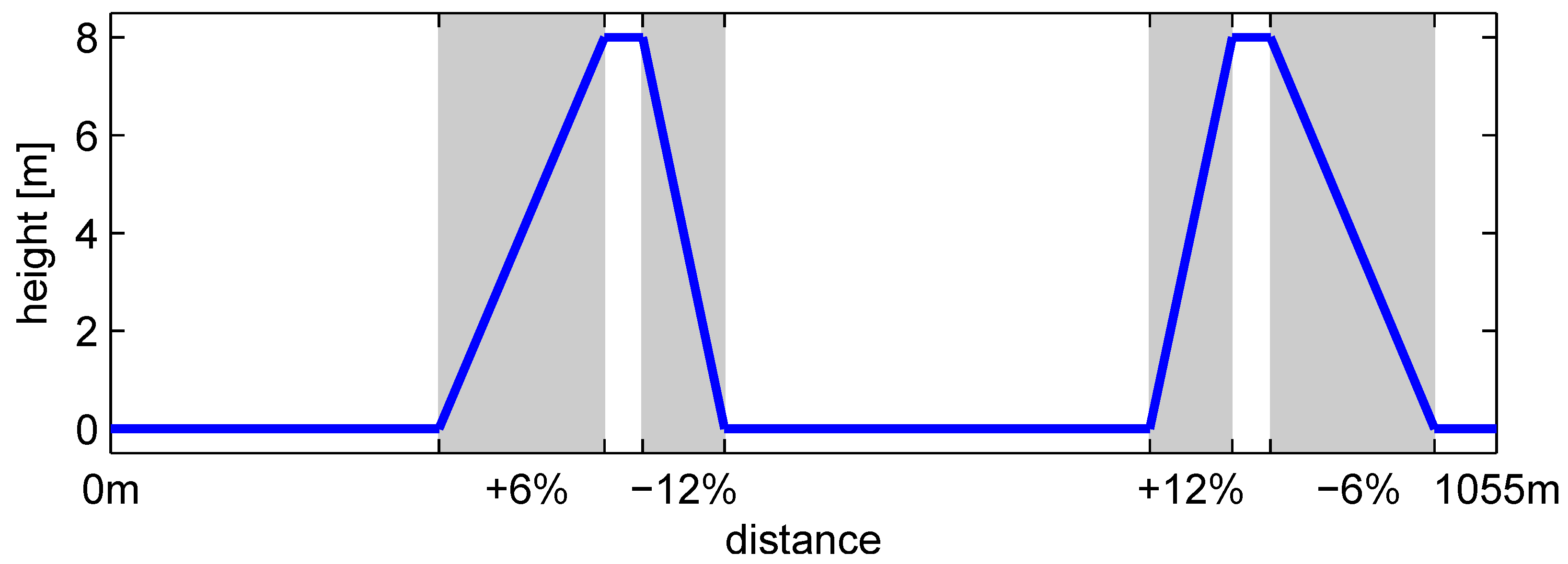
The first two scenarios are demonstrated for a cycle of 1055 m, with a vehicle weight of 25 tons. The elevation profile of this cycle is shown in Figure 16, and contains four slopes of respectively +6%, −12%, +12% and −6%. This elevation profile is also available as a physical test track as described in [28]. The maximum feasible speed on this track is 25 km/h. The plant model uses the models from Section 2, including the effect of open driveline during switching ().
The multi-level optimization is iteratively solved for the complete test cycle. Multiple iterations are performed; however, no decrease in fuel consumption is observed by consecutive iterations. The energy consumption of the first two iterations are shown in Table 7, where the energy consumption difference (0.1%) is negligible small. The control decisions of these two iterations are analyzed and compared in Appendix D and show that the calculated decisions after iteration 0, hardly change with iteration 1, with the difference in charge sustenance explaining the marginal change in energy consumption.
7.2. Multi-Level MPC, Short Cycle
For real-time applications, the Dynamic Program in Level 1 over the complete route is computationally too demanding. In this section, we simulate Level 1 as receding horizon optimization. Here, we choose to optimize Level 1 at a sample time of 1 s, with a horizon of five samples. The other levels are unaltered, as they don’t pose computational problems over the cycle’s horizon.
The energy consumption is marginally different (0.2%) from the other scenarios. The control decisions of the multi-level MPC are analyzed and compared with the multi-level iteration in Appendix E, showing equal decisions as the multi-level iteration. One essential difference in gear selection can be explained from the shorter horizon, however, without a relevant impact on energy consumption.
Comparing the three different scenarios, we conclude that the multi-level iteration scheme converges very fast: an update of the estimate of is not needed to improve the results of the optimizations on the layers, as iteration 0 is already at a minimal energy consumption. The multi-level MPC has a shorter horizon on Level 1, which leads to slightly different control decisions, but does not significantly alter the energy optimum. For fuel evaluation, the next section presents more realistic long-haul simulations, with the multi-level MPC implemented.
7.3. Multi-Level MPC, Long Cycle
To show the fuel saving potential of the multi-level EMS, a typical long-haul route is simulated, in which a non-hybrid vehicle is compared to a hybrid vehicle with baseline EMS (‘baseline’) and the multi-level MPC (‘preview’). The baseline EMS is a proprietary non-previewing, heuristic algorithm. The proprietary simulation environment is designed for fuel evaluation purposes and contains high-fidelity models of the vehicle. The multi-level MPC is implemented, with the following settings:
- Level 1, 5 s horizon, sample time 0.01 s,
- Level 2, 1000 s horizon, sample time 1 s,
- Level 3, 1000 s horizon, sample time 1 s.
For the 25-ton vehicle, the fuel consumption results are shown in Table 8.
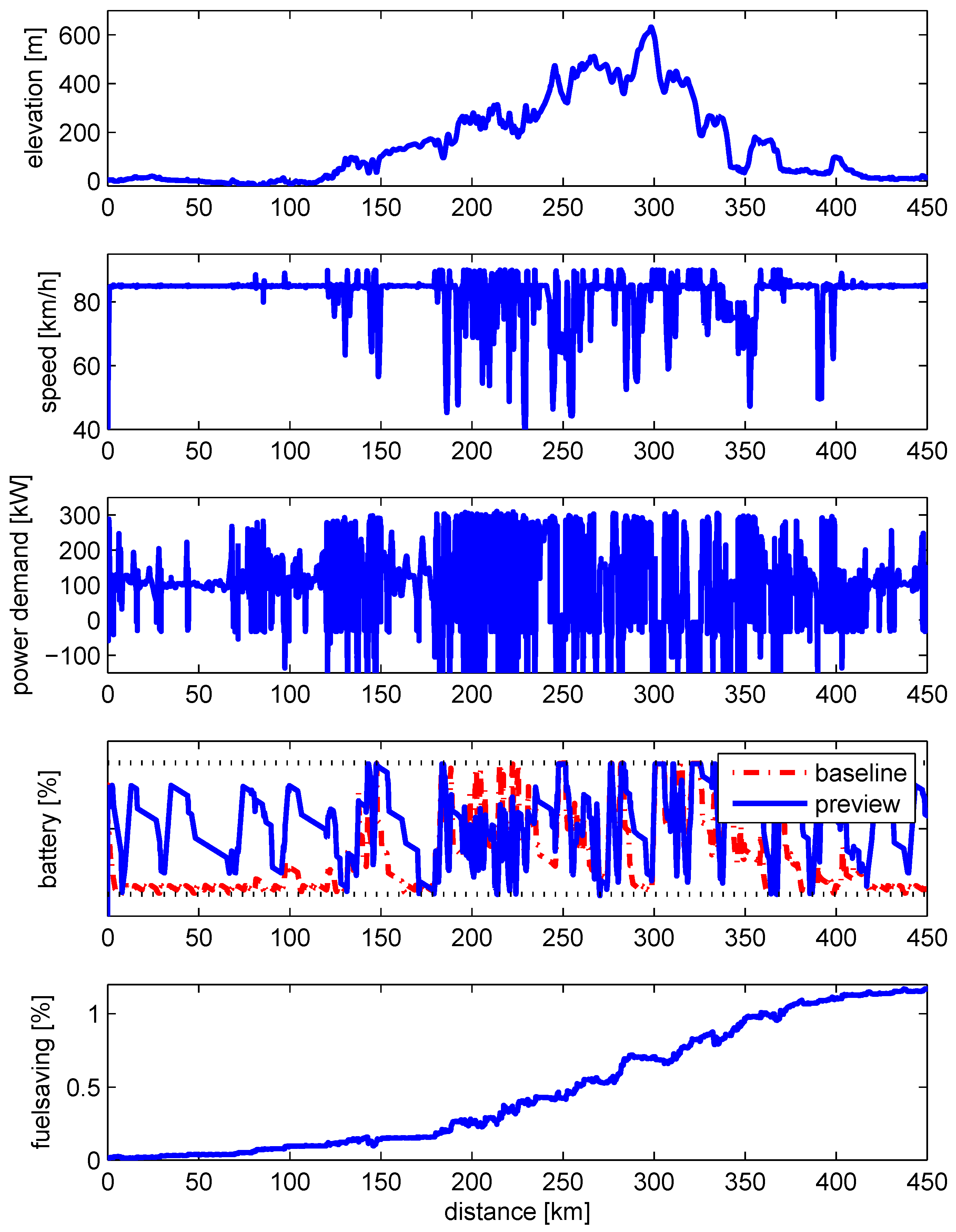
The difference between ‘baseline’ and ‘preview’ is best illustrated with the fuel saving and battery energy , plotted in Figure 17. There we observe the largest advantage of the previewing strategy, when battery limits are frequently touched, i.e., in the hilly part of the cycle: from 150–350 km. To recuperate a maximum amount of brake energy, ‘baseline’ discharges the battery as soon as possible, which is not the most efficient use of the recuperated energy. The previewing strategy discharges the battery sufficiently, to recuperate the maximum amount of brake energy, and uses the stored energy more efficiently, e.g., to drive MG-only during low road loads.
Also on segments without battery limitations, the previewing strategy outperforms the baseline strategy. On the flat road, e.g., from 0–120 km, coincides with guard (see Figure 9 and algorithm I3b in Section 5), resulting in fuel optimal switching control: charging the battery is performed in a relatively short period of time, shown by the steep increase of battery energy, followed by a prolonged period of a disconnected MG, thus eliminating MG friction . The baseline strategy, however, uses lower charging powers, thereby having little periods of MG disconnection, and thus higher MG friction. Furthermore, from a driveability perspective, the larger duty cycles of the previewing strategy, in connecting/disconnecting the MG, are preferred.
8. Conclusions
In this work, a computationally efficient EMS using preview is developed, obtaining excellent fuel economy results (−7.0%) on a typical long-haul route. To manage computational complexity, a multi-level EMS is designed, with on each level a specific algorithm for the subproblem to solve. Each subproblem uses different model information of the vehicle, such that optimal control techniques can be used, to efficiently solve the problem.
On level 1, the power-split, gear, mode decisions are optimized, including costs on switching. For the topology with two clutches, a novel explicit PMP solution is found, which reduces power-split and mode selection to a static calculation, dependent on the current vehicle state and battery costate (or Lagrange multiplier). For taking switching costs into account, a Dynamic Program is designed, using the explicit PMP solution for reducing the dimension of the problem, and thereby limiting the complexity of the calculations.
On level 2, the use of battery energy is optimized, taking the state constraints of the battery into account. A simpler, more abstracted vehicle model is used, e.g., by ignoring switching costs, to reduce computational complexity. Using PMP, the battery costate (or Lagrange multiplier) is calculated, which provides essential cost information to Level 1. The topology with two clutches, causes discrete jumps in the optimal solution, leading to non-unique (singular) solutions. New optimal solutions are found, minimizing the amount of switching events.
On level 3, the velocity is predicted along the route, using road slope and velocity limitations. With the calculation, essential route information is provided to the lower layers. Future work should include velocity optimization on this level, to further reduce the fuel consumption.
In offline simulation, on a short abstract drive cycle, the multi-level approach is shown to converge within one iteration. When the multi-level approach is used as Model Predictive Controller (MPC), comparable fuel energy efficiency is realized, even though the horizon is reduced.
Representative fuel saving results are obtained by running the multi-level MPC in a high fidelity simulation environment, over a typical heavy duty drive cycle: fuel reduction compared to a conventional vehicle, where the baseline EMS for the hybrid electric vehicle saves 5.8%.
Author Contributions
V.v.R. developed the presented concepts and methodologies. He performed writing and editing of the original draft. T.H. was responsible for supervision, internal reviewing and editing of the draft and concepts.
Funding
This research was funded by the Dutch Ministry of Economic Affairs, Agriculture and Innovation via the High Tech Automotive (HTAS) Program for the Hybrid Innovations for Trucks (HIT) project.
Acknowledgments
This research was supported by DAF Trucks N.V. and the Eindhoven University of Technology.
Conflicts of Interest
The authors declare no conflict of interest.
Appendix A. Pontryagin’s Minimum Principle
The Pontryagin’s Minimum Principle provides a set of equations (or conditions) where the optimal solution of a (constrained) dynamic optimization must comply to. Here, the PMP conditions are summarized, following [31,36]. For the fuel-cost functional:
with state equations given by:
the Hamiltonian is formulated:
where are the costates or Lagrange multipliers. For the optimal solution, it holds that
with the (Euler–Lagrange) necessary conditions:
where the superscript denotes the optimal solution. When the state is on a constraint at , is not defined and interior boundary conditions apply [37],
where the superscript and denote the left-hand side and right-hand side limit values, respectively, at . The conditions describe a possible jump condition in and H at , when the state makes contact with the boundary h. The magnitude of the jump is determined by the parameter , and is, together with the number of jumps, not known a priori. For the boundary conditions, additional transversality conditions hold, and are given (omitting the penalty on the final state) by:
Appendix B. Interpretation of the Costate
For the optimal control problem, the cost function J is minimized, which represents the total amount of fuel energy over a drive cycle:
with and
with x the state(s). Formulating the Hamiltonian leads to:
with the costate(s). Using the same variational approach used to derive the PMP conditions, the variation of the optimal J is defined as [31,36]:
which reveals the interpretation of at any time t: when and approach each other to t, the second term vanishes, and defines how much J changes, for a small change in x, i.e., is the gradient of the cost function, with respect to the states. This interpretation of is known as equivalent cost for the well known Equivalent Consumption Minimization Strategy [38], as it provides the equivalence (or price) between fuel energy and battery energy. When the same optimal control techniques are used in other EMS’s, e.g., considering more or different energy buffers, the interpretation of the costate is not always straightforward. Looking at the case of vehicle speed optimization as in [35,39], optimal control techniques lead to the optimal solution, but interpretation of is lacking. The reason is that, in these examples, the state is chosen to be velocity, which is not energy. If, however, the problem is reformulated with kinetic energy as state, see [40], the corresponding dynamics show valuable information. Thus, before is easily interpretable, the states of the problem should be reformulated as energies, as, e.g., in [8,9,40], where it is irrelevant if the reformulation is done before or after solving the problem. An example Hamiltonian of an energy minimizing function could be
with fuel energy , kinetic energy , battery energy , thermal energy and for the cycle duration. Then, by minimizing H, determines which energy buffer to charge and which energy buffer to deplete, thus being the buffers equivalency, or when the energy is valorized: price.
Appendix C. Cost of Switching
A switch of mode or gear involves a series of events, having some disadvantages, e.g.:
- synchronization of rotating masses (acceleration/deceleration), possibly with slipping clutches,
- interruption of traction.
The combination of these events determines the associated (fuel) cost of a mode/gear change event. The first item is defined by the design of the driveline itself and the low-level control of the event, and the energy losses can be calculated irrespective of the drive cycle, [19,41]. The second item is determined by the performance of the low-level control for the given hardware, namely the period of time traction is interrupted. Without traction, the vehicle is freewheeling, and dependent on the road load, will decelerate or accelerate. A cost can be associated with the lack of traction, dependent on the road load —for example driving uphill, interruption of traction is much more expensive than during cruising on a flat road. This second effect is not addressed by [41] or [19]. The novel approach here is to use cycle information from the velocity optimization, i.e., and (Appendix B), in order to account for the road load dependent switching cost.
The switch penalty is thereby divided into two parts: cost associated to synchronization, indicated with subscript s, and cost associated with traction interruption, indicated with subscript t, for both mode switches () and gear switches ():
Appendix C.1. Synchronization Cost
During a switch, rotating masses have to be accelerated and decelerated. Here, we assume:
- the largest cost is due to acceleration of rotation masses (inertia),
- during deceleration no energy is recuperated,
- switch events are typical, e.g., based on average behavior,
- each switch involves an inverse switch on a later moment.
The last assumption makes it possible to allocate an average cost to two linked events, e.g., starting the Combustion Engine (CE) has large costs associated, while stopping the CE is free. However, the one can not occur without the other, so the total cost of the two events can be averaged over the two single events. This results in balanced switch decisions in the EMS, when the horizon is small and only one of the linked events can be overseen within the horizon.
With the inertia from Table 3, the equivalent cost of the transitions are quantified with the change of rotational kinetic energy:
and translated to the equivalent fuel with:
which results in
with the inertia and speed just before () and after () the mode switch. As defines the fuel equivalence between electrical and thermal energy, it is not relevant with which energy source the synchronization is performed. For example, an ICE start first involves an electrical acceleration, followed by mechanical acceleration as soon as the rotational speed is above idle speed, but, with , they are equivalent. The same method is used to calculate .
For the following rotational speeds,
- disconnected, stopped: 0 rpm,
- connected: 930 rpm,
- downshift: 1200 rpm,
the equivalent costs (here: ) are exemplified in Table A1. The downshift event losses depend on the active mode, respectively , , and , because losses increase with the amount of rotational mass to be accelerated, which is the largest with both CE and MG connected. The transitions involving deceleration of the rotational masses are set to 0. However, some energy recuperation could be implemented with the MG, resulting in lower average equivalent costs.

Table A1.
Equivalent cost of transition: synchronisation.
| Transition | Direction ⇒ [kJ] | Direction ⇐ [kJ] | Avg [kJ] |
|---|---|---|---|
| 0 | 10,20,30 | 20 | |
| 16 | 31 | 24 | |
| 16 | 0 | 8 | |
| 31 | 0 | 16 |
It should be noted that the transitions are idealized. The real energy consumption of the transitions will be worse than the posed numbers due to additional losses but can be improved by recuperation on the decelerating masses. Nevertheless they provide a first estimate on the selection of , which has clear mode dependent values. For a more thorough analysis of the gear switch event, including clutch slip, see [41] (Chapter 6).
Appendix C.2. Traction Interruption Cost
During the transition of a switch, the traction is momentarily interrupted. This interruption causes a deviation from the intended vehicle speed, which has to be compensated during the periods with traction. Dependent on the road load, the cycle and the component capabilities, this compensation is expensive or cheap. The idea here is to quantify the cost of this compensation to the cycle through the information contained in the costates belonging to the cycle: in Equation (A14). To link this information to the traction interruption cost, the following idealized transition is assumed:
- the transition has a fixed traction interruption time (),
- during the transition, the road load is constant,
- the driveline is not saturated, i.e., traction is available to recover the vehicle speed,
- represents the equivalent cost of time loss for a certain cycle, and is constant.
In Figure A1, the idealized transition is plotted. While cruising at , where , a switch event is planned at . During the following open driveline period –, constant deceleration causes the vehicle speed to drop. After the transition, we assume immediate recovery to the desired speed, with constant acceleration at , depending on the mode M and associated component capabilities. During this event, the vehicle loses time, with respect to cruising without transition. If we compare the total transition+recovery time to reach the position at , with the time needed for constant cruising to reach position , we define the time loss of the transition event:
with
This time loss is converted to equivalent fuel, with , thus providing a road load dependent penalty on switching,
When the drive-line saturates (), the vehicle is not able to recover the cruise speed after a short open driveline event. In that situation, the speed deviation is used with to calculate the speed recovery cost. The same method is used to calculate .
As an example the equivalent cost of a transition due to time loss is given in Table A2, for the model parameters from Table 3, the vehicle driving 25 km/h, and the cycle having a of kJ/s. The event is tabulated for three segments of, respectively, 0%, 6% and 12% slope. The traction interruption period is set to 1 s.
Table A2 shows that more than a magnitude order of difference occurs for a switch cost. This means that the influence of time loss on the equivalent fuel consumption is relevant when the open driveline deceleration (acceleration) is high, where on other route segments the influence is negligible. This shows that transitions can be best planned during the segments with smallest deceleration (acceleration).
The switch cost is now determined by two elements: synchronization cost as a function of the intended transition, and time loss cost as a function of position along a route and the available traction for the transition, in Equations (A15) and (A16).
Figure A1.
Open driveline behavior for timeloss () calculation. From to , no traction is available, causing the vehicle to decelerate. From to , speed recovery takes place at maximum traction . Arrival at position is later than without switch event (dotted line), which is the defined timeloss.
Figure A1.
Open driveline behavior for timeloss () calculation. From to , no traction is available, causing the vehicle to decelerate. From to , speed recovery takes place at maximum traction . Arrival at position is later than without switch event (dotted line), which is the defined timeloss.
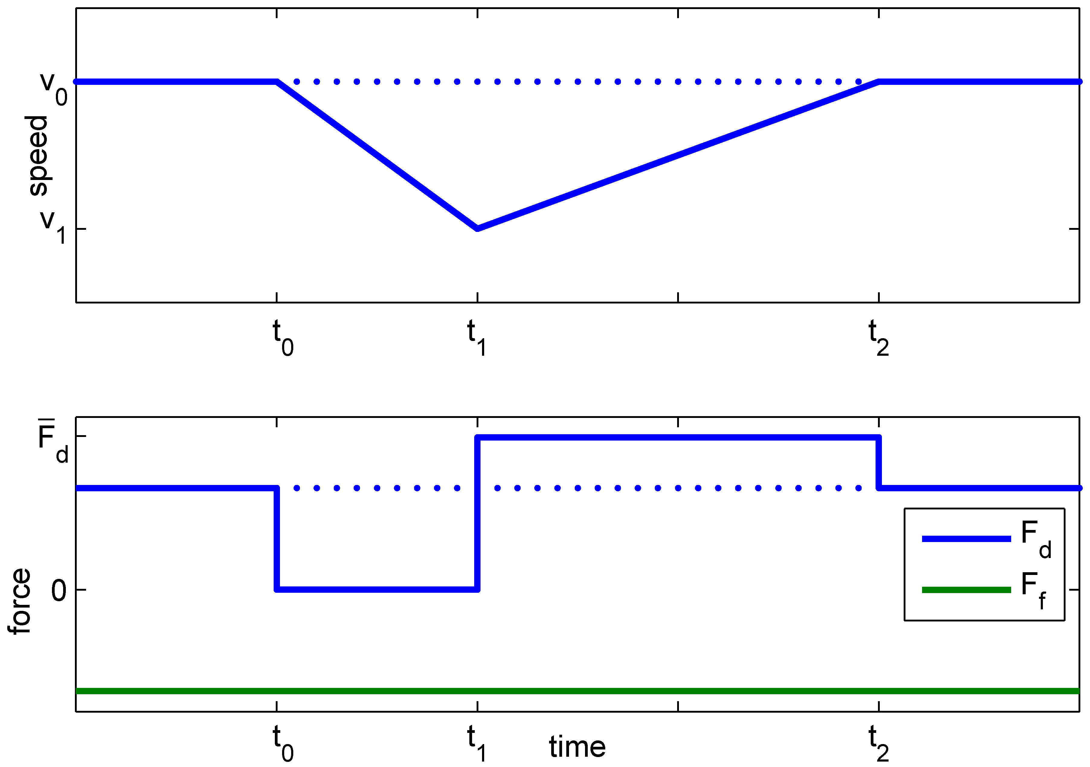
Table A2.
Equivalent cost of time loss due to a switch event of 1 s.
| Segment | Timeloss [s] | Speedloss [m/s] | Eq. Cost [kJ] |
|---|---|---|---|
| 0% | −0.01 | −0.075 | 0.17 |
| 6% | −0.07 | −0.65 | 1.8 |
| 12% | −0.22 | −1.25 | 5.6 |
Appendix D. Simulation Results of Multi-Level Iteration
For the simulation on the short drive cycle, multiple iterations are performed in the multi-level EMS of this work. In this section, the decisions of the first two iterations are analyzed, illustrating the fast convergence of the algorithm.
Appendix D.1. Iteration 0
In the zeroth iteration, each level is optimized consecutively, starting at Level 3. The assumptions in each Level are described:
- Level 3: on this level, we assume that the vehicle is cruising constantly at the maximum speed , i.e., 25 km/h. The elevation is given by Figure 16. Assuming an average, constant engine speed (here: 1100 rpm), is calculated.
- Level 2: on this level, charge sustenance is enforced () by searching for . The capabilities of the CE and MG at 1100 rpm influence the resulting power-split and mode switching.
- Level 1: on this level, the cost of switching is added to the power-split optimization, using the just found , and . The resulting dynamic program is solved for the full horizon, here 10.6 km.
In Figure A2, the result is shown for respectively MG power (), mode (M), gear (G), battery energy () and vehicle speed (v). The top plot also includes (dotted black) as a reference. On the flat segments, kW and on the slopes kW for, respectively, the +6%, −12%, +12% and −6% segment. The dashed lines indicate the decisions of Level 2, the solid lines of Level 1.
Figure A2.
Decisions and results from Level 2 and 1, after the zeroth iteration. Due to the different model abstraction, the solution on Level 1 is not exactly charge sustaining anymore.
Figure A2.
Decisions and results from Level 2 and 1, after the zeroth iteration. Due to the different model abstraction, the solution on Level 1 is not exactly charge sustaining anymore.
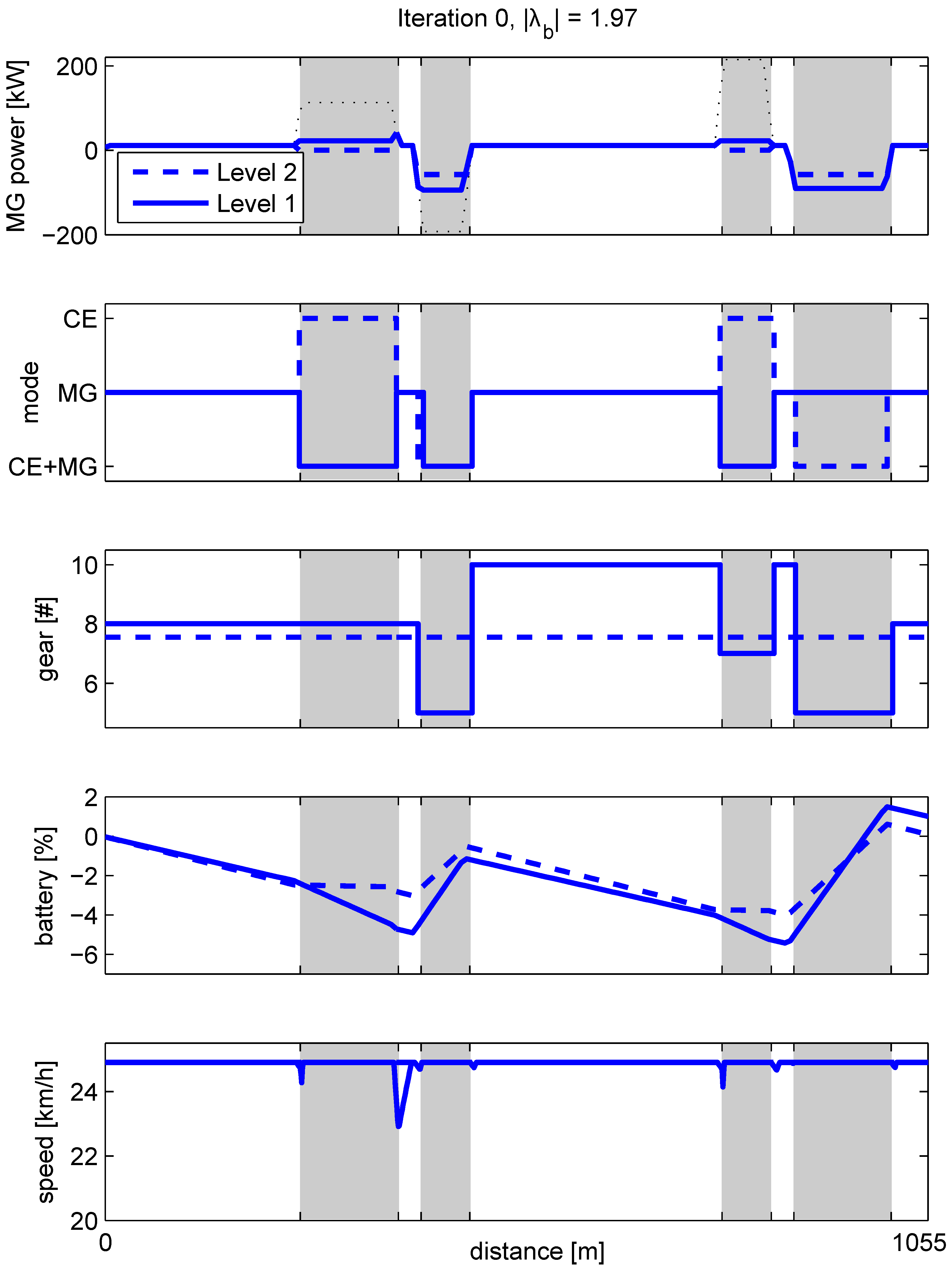
Level 2 (dashed line) calculates a charge sustaining , shown in subplot 4, where starts and ends at 0. It uses a simplified model which keeps the engine speed at 1100 rpm, showing in subplot 3 as a selected gear between 7 and 8. At this engine speed, it is optimal to drive the flat segments in MG mode (), with the CE switched off. The uphill segments have higher power demands , and the CE is used. On the downhill segments, brake energy is recuperated with the MG, but the CE must assist in braking, as is larger than the MG can recuperate. As all switches are assumed to be infinitely fast, the bottom plot shows no speed deviation for Level 2.
Level 1 (solid line) uses and the switching costs to determine the optimal mode and gear switching sequence. Most importantly, the gear on the downhill segments is shifted down to 5, in order to maximize the recuperation power of the MG (see Figure 3), which is notable by an increased rise in energy of the battery for these segments. Due to the downshift, the −6% can be driven with the MG alone. The −12% still needs both MG and CE for additional braking power. The uphill segments show a different mode selection than for Level 2. From the control map, we know that is close to the guard , where the Hamiltonian of is only slightly lower than of , causing Level 2 to decide for . Level 1, however, takes the switching costs into account, and where both levels decide to start and stop the CE, Level 1 decides that stopping and starting the MG is more expensive than the minor fuel advantage of the lower Hamiltonian, resulting in mode with 22 kW boosting of the MG. Gear selection on the flat segments is towards the highest possible gear where the MG is able to deliver the demanded power, thereby minimizing the friction of the MG.
Due to the switching of mode and gear, several open driveline events occur. The cost of timeloss, as calculated in Section 4.3, determines that, if a switch is needed, it should be done where the timeloss is minimal. For this cycle, this is clearly on the flat segments, not on any of the slopes. This results in only minor vehicle speed deviations in the vehicle speed.
Due to the different control actions between Level 1 and Level 2, charge sustenance is not enforced anymore. This is to be corrected in the next iteration.
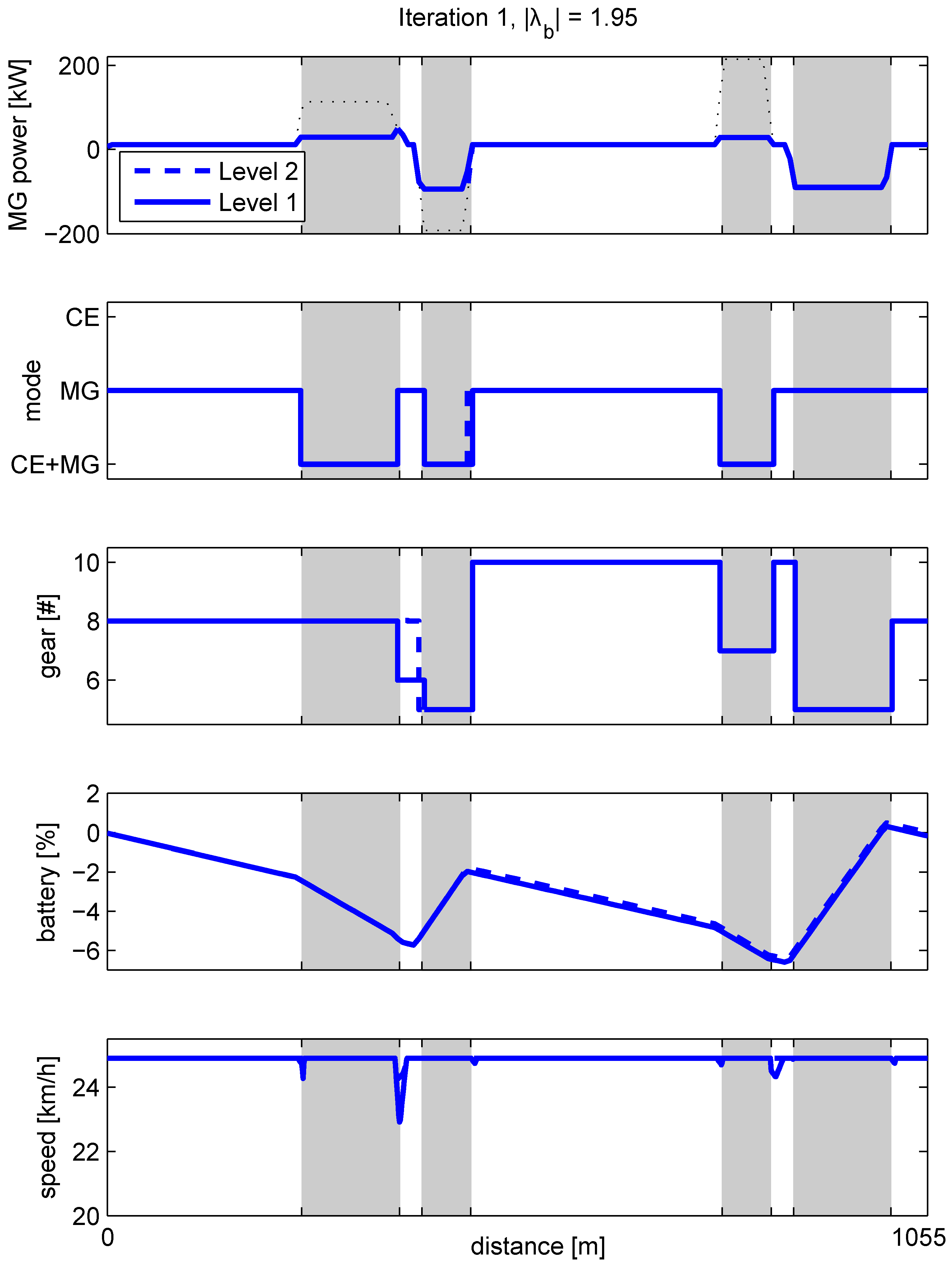
Appendix D.2. Iteration 1
In the first iteration, each control level is optimized consecutively, using the results from the zeroth iteration. The differences with the zeroth iteration are:
- Level 3: the constant engine speed from iteration 0 is replaced by the speed resulting from the gear switching sequence. As speed is not explicitly optimized and can always be maintained in this example, is not altered.
- Level 2: using the gear switching sequence, a new charge sustaining is calculated.
- Level 1: with the adjusted , the power-split and switching sequence are optimized
In Figure A3, the results are shown for Level 2 and Level 1 for the first iteration. It is evident that no significant differences are present between the two levels. An additional gear shift occurs on the top of the first hill, but, as the friction of the MG at different speeds is very small, the fuel advantage is negligible. Comparing to iteration 0, the difference with Level 2 of iteration 0 is also very small. The main effect of the iteration is that the cycle is charge sustaining again, with . To realize that, the boosting power of the MG is slightly increased from 22 kW to 29 kW on the uphill slopes.
Figure A3.
Decisions and results from Level 2 and 1, after the first iteration. After updating the information on and , the solution on both levels converges, and are charge sustaining.
Figure A3.
Decisions and results from Level 2 and 1, after the first iteration. After updating the information on and , the solution on both levels converges, and are charge sustaining.

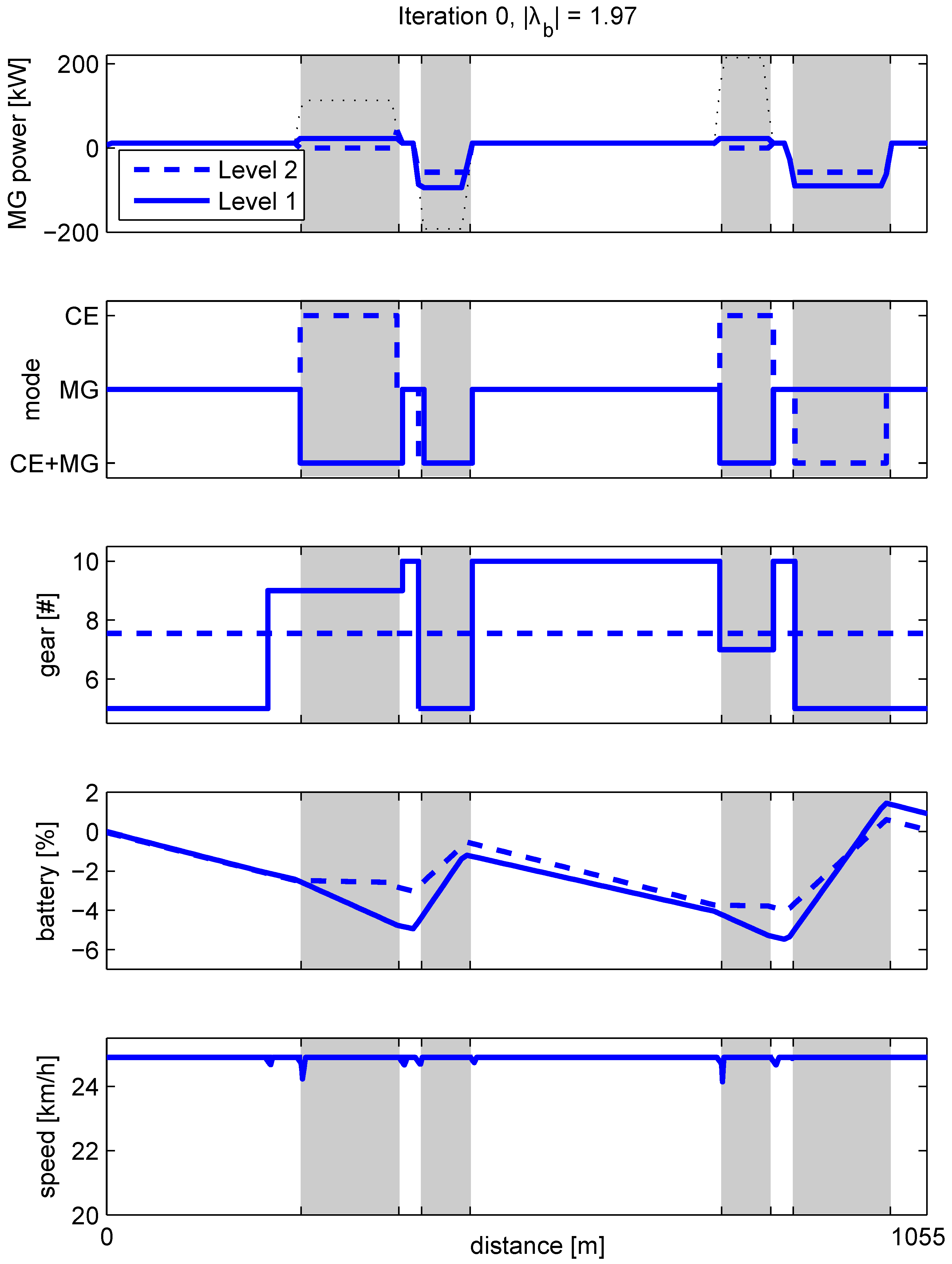
Appendix E. Simulation Results of Multi-Level MPC
In Figure A4, the results are shown for Level 2 and Level 1 for the first iteration. As Level 2 is not changed, the Level 2 traces are the same as in Figure A2. Albeit Level 1 now has a horizon of 5 s, instead of 10 km, the mode decisions are unaltered. However, the gear decisions differ in some segments:
- the trace starts at and is maintained for a long time. That gear is selected at the end of the −6% slope to maximize brake energy recuperation. After the slope, is low, and a little friction reduction of the MG could be accomplished with an upshift. However, the fuel improvement of switching in MG is an order of magnitude lower than in other modes. Now, for a gear switch to occur, the accumulated fuel improvement over the horizon (5 s) must be higher than the cost of the switch event itself, which it is not, for this short horizon, and the switch will not occur.
- on the +6%, a higher gear is needed, in order to minimize CE friction losses. Before the +6% slope, this decision enters the horizon, and, as the switch will be made anyhow, the algorithm decides to do the switch immediately, as driving MG in is slightly more profitable.
- on the top of the first hill, a short shift to is performed, simultaneously with a mode switch, which makes the gear switch event cheap. The decision has, however, a marginal impact on the fuel consumption.
Figure A4.
Results for MPC, with a 5-sample horizon on Level 1. Differences with Figure A2 are mainly in the gear decisions, with a marginal impact on fuel.
Figure A4.
Results for MPC, with a 5-sample horizon on Level 1. Differences with Figure A2 are mainly in the gear decisions, with a marginal impact on fuel.
References
- Sciarretta, A.; Guzzella, L. Control of hybrid electric vehicles. IEEE Control Syst. Mag. 2007, 27, 60–70. [Google Scholar]
- Serrao, L. Open Issues in Supervisory Control of Hybrid Electric Vehicles: A unified approach using optimal control methods. In Proceedings of the RHEVE Hybrid and Electric Vehicles, Paris, France, 6–7 December 2011. [Google Scholar]
- Willems, F.; Spronkmans, S.; Kessels, J. Integrated Powertrain Control to meet low CO2 emissions for a hybrid distribution truck with SCR-deNOx system. In Proceedings of the Dynamic Systems and Control Conference, Arlington, VA, USA, 31 October–2 November 2011. [Google Scholar]
- Pham, T.; Kessels, J.; van den Bosch, P.; Huisman, R. Integrated Energy and Thermal Management for Hybrid Electric Heavy Duty Trucks. In Proceedings of the IEEE Vehicle Power and Propulsion Conference, Seoul, Korea, 9–12 October 2012. [Google Scholar]
- van Reeven, V.; Huisman, R.; Kessels, J.; Pham, T.; Hofman, T. Integrating energy and thermal management of hybrid trucks. In Proceedings of the VDI Commercial Vehicles, Celle, Germany, 5–6 June 2013. [Google Scholar]
- Donkers, M.; Schijndel, J.V.; Heemels, W.; Willems, F. Optimal control for integrated emission management in diesel engines. Control Eng. Pract. 2017, 61, 206–216. [Google Scholar] [CrossRef] [Green Version]
- Willems, F.; Kupper, F.; Rascanu, G.; Feru, E. Integrated Energy and Emission Management for Diesel Engines with Waste Heat Recovery using Dynamic Models. Oil Gas Sci. Technol. 2015, 70, 143–158. [Google Scholar] [CrossRef]
- van Reeven, V.; Hofman, T.; Willems, F.; Huisman, R.; Steinbuch, M. Optimal control of engine warmup in hybrid vehicles. Oil Gas Sci. Technol. 2014, 71, 14. [Google Scholar] [CrossRef]
- Merz, F.; Sciarretta, A.; Dabadie, J.C.; Serrao, L. On the optimal thermal management of hybrid-electric vehicles with heat recovery sytems. Oil Gas Sci. Technol. 2012, 67, 601–612. [Google Scholar] [CrossRef]
- Back, M. Pradiktive Antriebsregelung zum Energieoptimalen Betrieb von Hybridfahrzeugen. Ph.D. Thesis, Universitat Fridericiana Karlsruhe, Karlsruhe, Germany, 2005. [Google Scholar]
- Johannesson, L.; Asbogard, M.; Egardt, B. Assessing the Potential of Predictive Control for Hybrid Vehicle Powertrains Using Stochastic Dynamic Programming. IEEE Trans. Intell. Transp. Syst. 2007, 8, 71–83. [Google Scholar] [CrossRef]
- Delprat, S.; Guerra, T.; Paganelli, G.; Lauber, J.; Delhom, M. Control strategy optimization for a hybrid parallel powertrain. In Proceedings of the 2001 American Control Conference, Arlington, VA, USA, 25–27 June 2001. [Google Scholar]
- Finkeldei, E.; Back, M. Implementing an MPC algorithm in a vehicle with a hybrid powertrain using telematics as a sensor for powertrain control. In Proceedings of the IFAC Symposium on Advances in Automotive Control, Arlington, VA, USA, 25–27 June 2004. [Google Scholar]
- Borhan, H.; Vahidi, A.; Phillips, A.; Kuang, M.; Kolmanovsky, I.; Cairano, S.D. MPC-Based energy Management of a power-split hybrid electric vehicle. IEEE Trans. Control Syst. Technol. 2012, 20, 593–603. [Google Scholar] [CrossRef]
- Ambühl, D.; Sundström, O.; Sciarretta, A.; Guzzella, L. Explicit optimal control policy and its practical application for hybrid electric powertrains. Control Eng. Pract. 2010, 18, 1429–1439. [Google Scholar] [CrossRef]
- Murgovski, N.; Johannesson, L.M.; Sjöberg, J. Engine on/off control for dimensioning hybrid electric powertrains via convex optimization. IEEE Trans. Veh. Technol. 2013, 62, 2949–2962. [Google Scholar] [CrossRef]
- Elbert, P. Noncausal and Causal Optimization Strategies for Hybrid Electric Vehicles. Ph.D. Thesis, ETH Zurich, Zurich, Switzerland, 2013. [Google Scholar]
- Ngo, V.; Hofman, T.; Steinbuch, M.; Serrarens, A. Optimal Control of the Gear Shift Command for Hybrid Electric Vehicles. IEEE Trans. Veh. Technol. 2012, 61, 3531–3543. [Google Scholar] [CrossRef]
- Nüesch, T.; Elbert, P.; Flankl, M.; Onder, C.; Guzzella, L. Convex optimization for the energy management of hybrid electric vehicles considering engine start and gearshift costs. Energies 2014, 7, 834–856. [Google Scholar] [CrossRef]
- van Reeven, V.; Hofman, T.; Huisman, R.; Steinbuch, M. Extending Energy Management in Hybrid Electric Vehicles with Explicit Control of Gear Shifting and Start-Stop. In Proceedings of the American Control Conference, Montreal, QC, Canada, 27–29 June 2012. [Google Scholar]
- Scattolini, R. Architectures for distributed and hierarchical model predictive control. J. Process Control 2009, 19, 723–731. [Google Scholar] [CrossRef]
- Ambühl, D.; Guzzella, L. Predictive Reference Signal Generator for Hybrid Electric Vehicles. IEEE Trans. Veh. Technol. 2009, 58, 4730–4740. [Google Scholar] [CrossRef]
- van Keulen, T.; Jager, B.d.; Serrarens, A.; Steinbuch, M. Optimal Energy Management in Hybrid Electric Trucks Using Route Information. Oil Gas Sci. Technol. Rev. IFP 2010, 65, 103–113. [Google Scholar] [CrossRef]
- Sun, C.; Moura, S.J.; Hu, X.; Hedrick, J.K.; Sun, F. Dynamic Traffic Feedback Data Enabled Energy Management in Plug-in Hybrid Electric Vehicles. IEEE Trans. Control Syst. Technol. 2015, 23, 1075–1086. [Google Scholar]
- Mesarovic, M.D.; Macko, D.; Takahara, Y. Theory of Hierarchical Multilevel Systems; Academic Press: Cambridge, MA, USA, 1970. [Google Scholar]
- Maciejowski, J. Predictive Control with Constraints; Prentice Hall: Upper Saddle River, NJ, USA, 2002. [Google Scholar]
- Findeisen, W. Control and Coordination in Hierarchical Systems; John Wiley & Sons: Hoboken, NJ, USA, 1980. [Google Scholar]
- Van Reeven, V.; Hofman, T. Multi-level energy management: Implementation and validation—Part II. Vehicles 2018. under review. [Google Scholar]
- Guzzella, L.; Onder, C. Introduction to Modeling and Control of Internal Combustion Engine Systems; Springer: Berlin, Germany, 2010. [Google Scholar]
- Bialas, W.F.; Karwan, M.H. Multilevel Linear Programming; State University of New York: Buffalo, NY, USA, 1978; p. 78-1. [Google Scholar]
- Kirk, D.E. Optimal Control Theory, an Introduction; Dover Publications: Chicago, IL, USA, 1970. [Google Scholar]
- van Keulen, T.; Gillot, J.; de Jager, B.; Steinbuch, M. Solution for state constrained optimal control problems applied to power split control for hybrid vehicles. Automatica 2014, 50, 187–192. [Google Scholar] [CrossRef]
- Wei, X.; Utkin, V.; Rizzoni, G.; Guzzella, L. Model-based Fuel Optimal Control of Hybrid Electric Vehicle using Variable Structure Control Systems. J. Dyn. Syst. Meas. Control 2007, 129, 13–20. [Google Scholar] [CrossRef]
- Delprat, S.; Hofman, T. Hybrid Vehicle Optimal Control: Linear Interpolation and Singular Control. In Proceedings of the IEEE Vehicle Power and Propulsion Conference, Coimbra, Portugal, 27–30 October 2014. [Google Scholar]
- Fröberg, A.; Nielsen, L. Optimal Control Utilizing Analytical Solution for Heavy Truck Cruise Control; Internal Report; Linkopings Universitet: Linkoping, Sweden, 2008. [Google Scholar]
- Bryson, A.E.; Ho, Y. Applied Optimal Control; Taylor and Francis: Abingdon, UK, 1975. [Google Scholar]
- Hartl, R.F.; Sethi, S.P.; Vickson, R.G. A survey of the maximum principle for optimal control problems with state constraints. SIAM 1995, 37, 181–218. [Google Scholar] [CrossRef]
- Sciarretta, A.; Back, M.; Guzzella, L. Optimal control of parallel hybrid electric vehicles. IEEE Trans. Control Syst. Technol. 2004, 12, 352–363. [Google Scholar] [CrossRef]
- van Keulen, T.; de Jager, B.; Foster, D.; Steinbuch, M. Velocity Trajectory Optimization in Hybrid Electric Trucks. In Proceedings of the American Control Conference, Baltimore, MD, USA, 30 June–2 July 2010. [Google Scholar]
- Hellström, E.; Åslund, J.; Nielsen, L. Horizon length and fuel equivalents for fuel-optimal look-ahead control. In Proceedings of the Advances in Automotive Control, Munich, Germany, 12–14 July 2010. [Google Scholar]
- Ngo, V. Gear Shift Strategies for Automotive Transmissions. Ph.D. Thesis, Technical University Eindhoven, Eindhoven, The Netherlands, 2012. [Google Scholar]
Figure 1.
Multi-level optimization of the velocity (v), battery energy () and power split () including mode and gear selection (). In Section 3 the scheme is described, with the prediction of: road slope (), velocity limit (), driveline rotational speed (), driveline power (), velocity () and battery costate (), dependent on: vehicle position (s), velocity (v), battery energy (), driveline power (), mode (M) and gear (G).

Figure 2.
Topology of the parallel Hybrid Electric Vehicle with its relevant power flows, defined positive towards the road and relevant states (between parenthesis).
Figure 2.
Topology of the parallel Hybrid Electric Vehicle with its relevant power flows, defined positive towards the road and relevant states (between parenthesis).

Figure 3.
Power capabilities of internal combustion engine (CE) and motor generator (MG) as a function of the rotational speed. Dotted lines indicate the nominal friction and .
Figure 3.
Power capabilities of internal combustion engine (CE) and motor generator (MG) as a function of the rotational speed. Dotted lines indicate the nominal friction and .
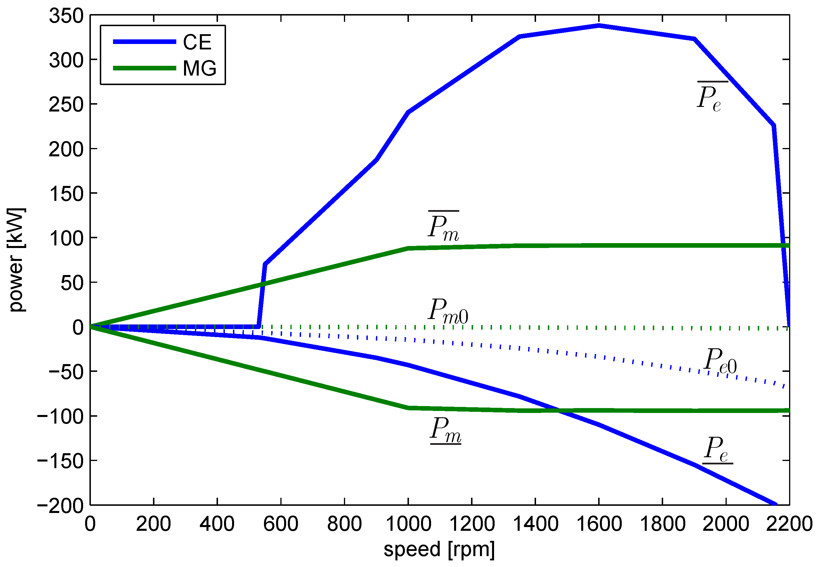
Figure 4.
State machine for switching between modes M. All mode switches go through (‘open driveline’), which is maintained for . The negation of the mode command is denoted with .
Figure 4.
State machine for switching between modes M. All mode switches go through (‘open driveline’), which is maintained for . The negation of the mode command is denoted with .
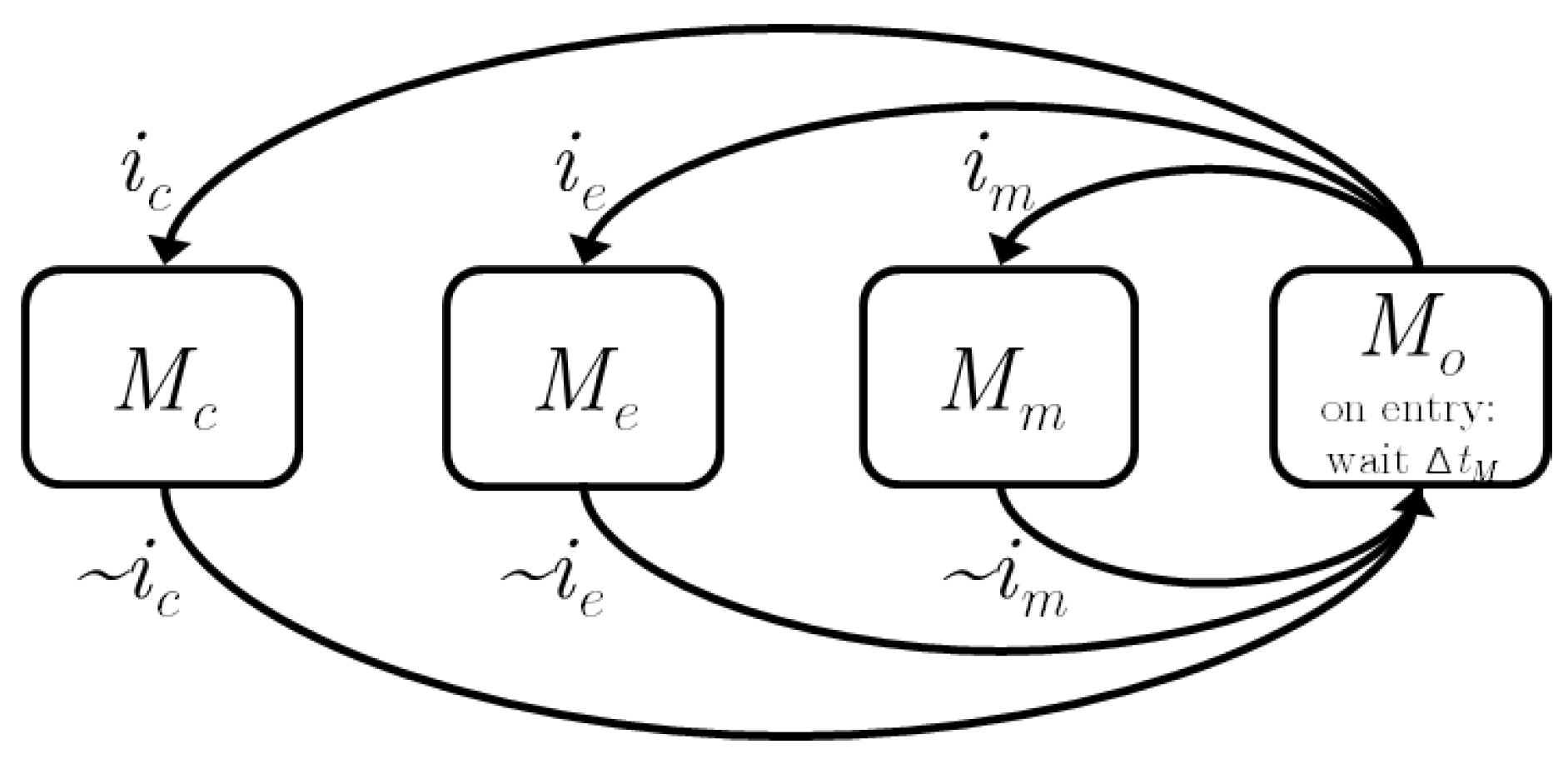
Figure 5.
State machine for switching between gears G. All gear switches go through (‘open driveline’), which is maintained for . The negation of the gear command is denoted with .
Figure 5.
State machine for switching between gears G. All gear switches go through (‘open driveline’), which is maintained for . The negation of the gear command is denoted with .
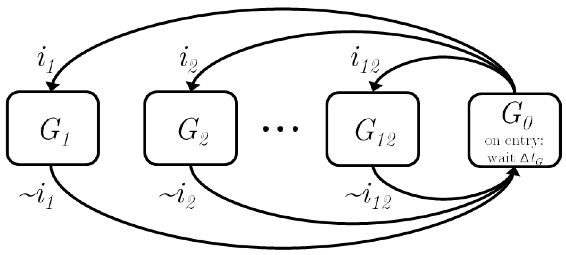
Figure 6.
Schematic of the horizon in the ‘multi-level iteration’ and ‘multi-level Model Predictive Controller (MPC)’ solution schemes. The multi-level iteration has an identical horizon, for all levels, and for all iterations, comprising the complete drive cycle. The multi-level MPC has a solution scheme, with shorter horizon lengths. With each time sample, the vehicle moves along the drive cycle. At each time sample, one iteration is performed, over a horizon starting at , having a fixed horizon length to . When the level has a faster sample time, iterations are performed more often, thereby improving the feedback performance.

Figure 7.
The Hamiltonian of the three modes as a function of for a power demand and rotational speed. The optimal mode changes at the boundary points .
Figure 7.
The Hamiltonian of the three modes as a function of for a power demand and rotational speed. The optimal mode changes at the boundary points .
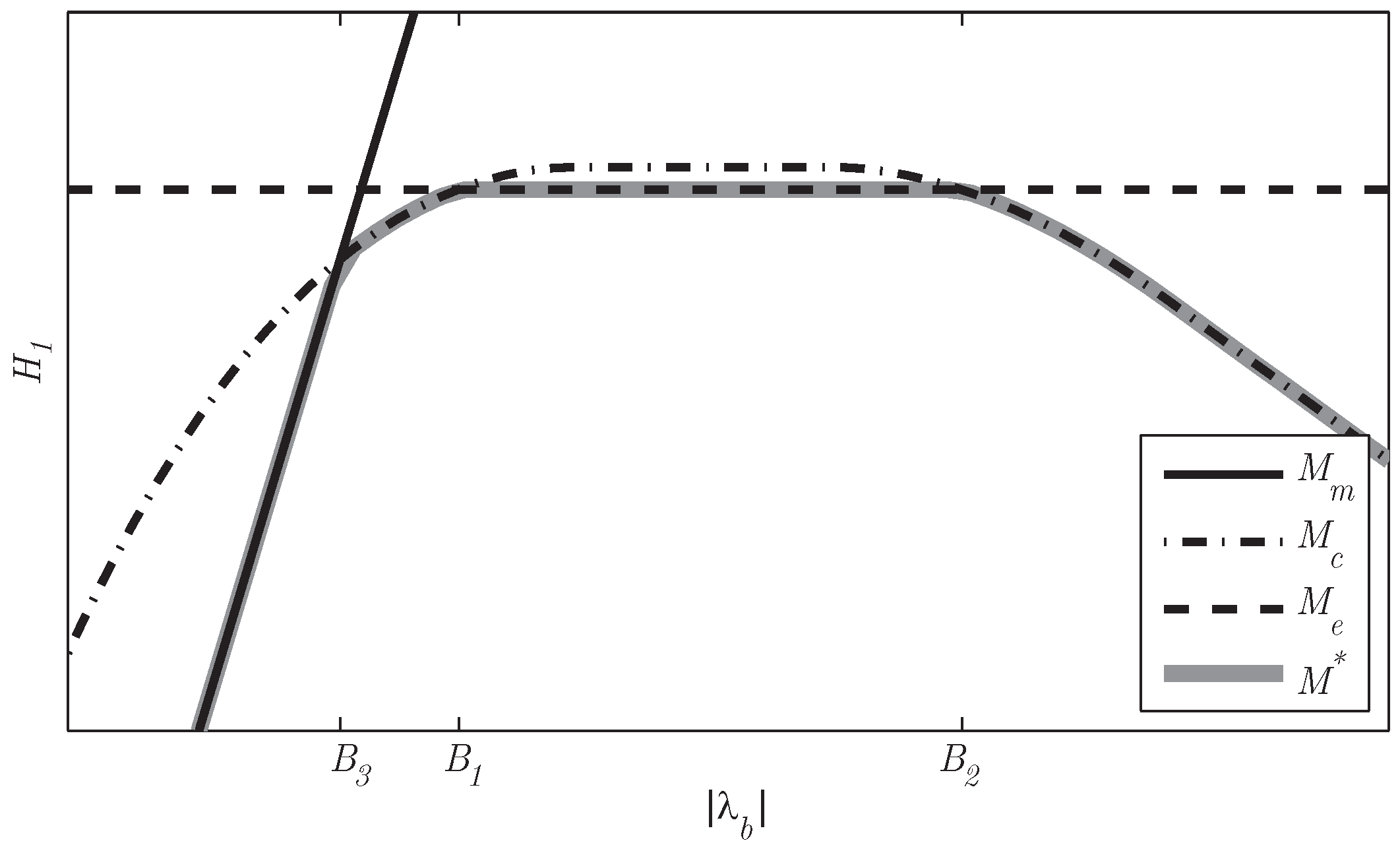
Figure 8.
as a function of for the modes for a power demand and gear. At and , the optimal mode switches between and , with a corresponding jump in . At a jump occurs due to switching between and .
Figure 8.
as a function of for the modes for a power demand and gear. At and , the optimal mode switches between and , with a corresponding jump in . At a jump occurs due to switching between and .
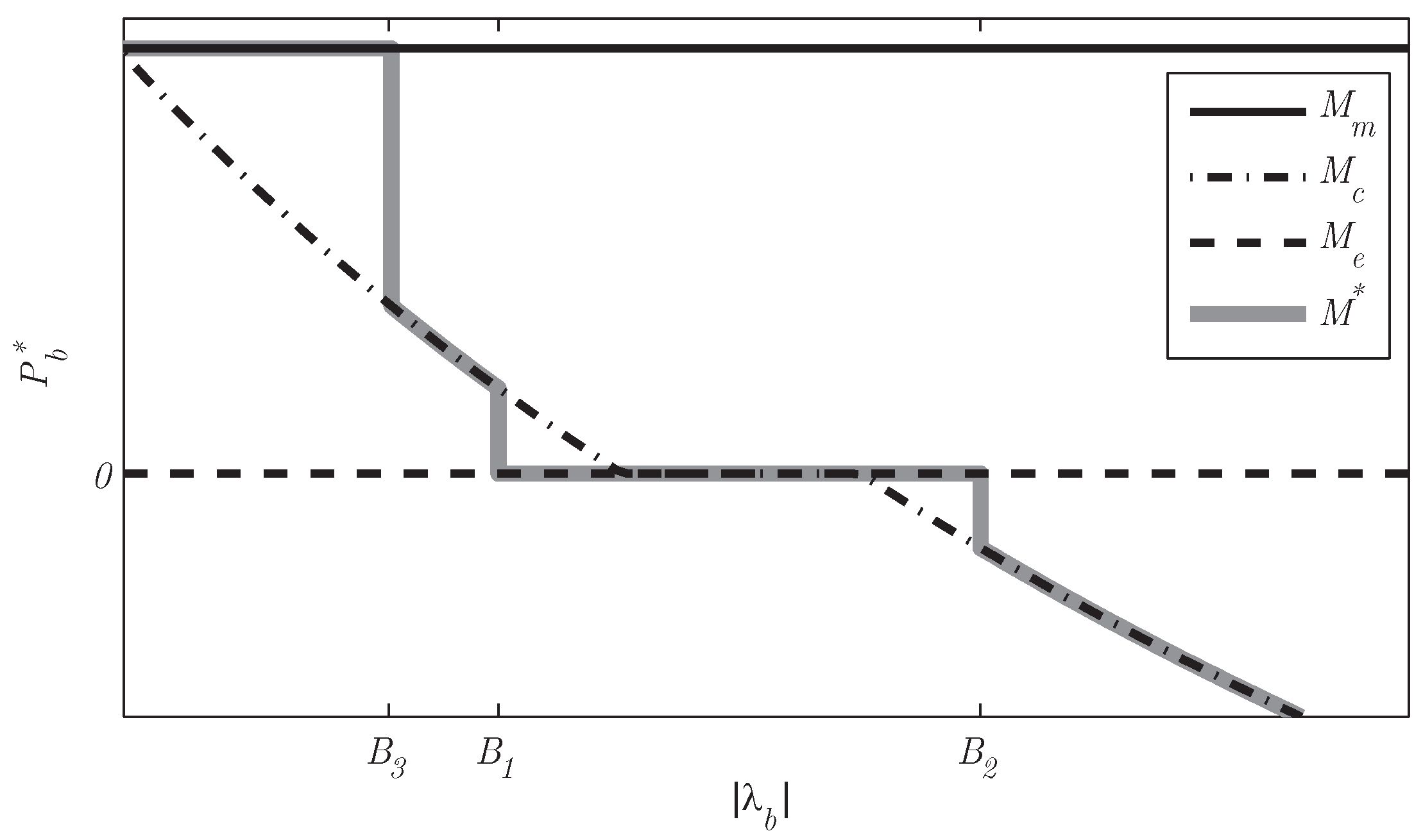
Figure 9.
Explicit mode change map as a function of costate and power demand , indicating the guards B between the optimal modes (motor-only), (engine-only) and (combined). Figure 7 and Figure 8 are cross sections at .
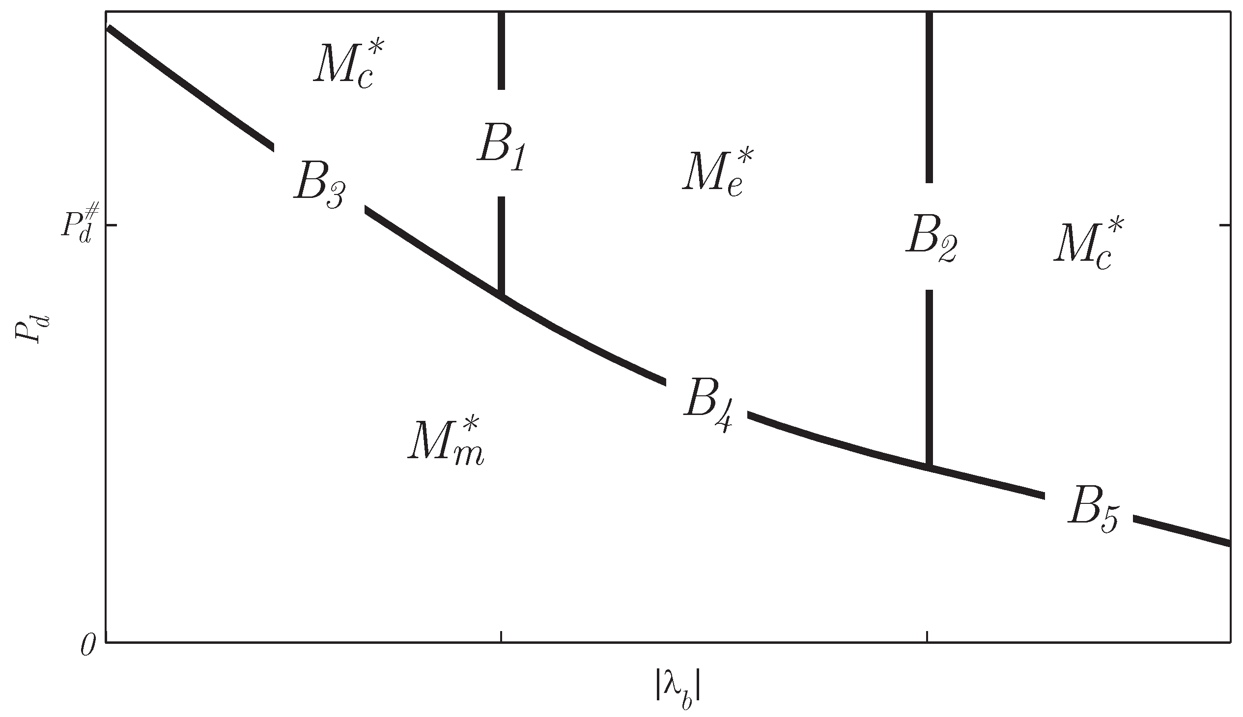
Figure 10.
Illustrating the Receding Horizon Integer Program to solve at each time step. Over a horizon of four seconds with a sampling time of one second, all feasible modes and gears are enumerated (blue), starting at the current mode and gear (red). For all feasible modes, H is calculated, increased with an equivalent fuel penalty on each mode or gear change, and the optimal trajectory over the horizon (blue dotted line) is determined, using Dynamic Programming (DP).
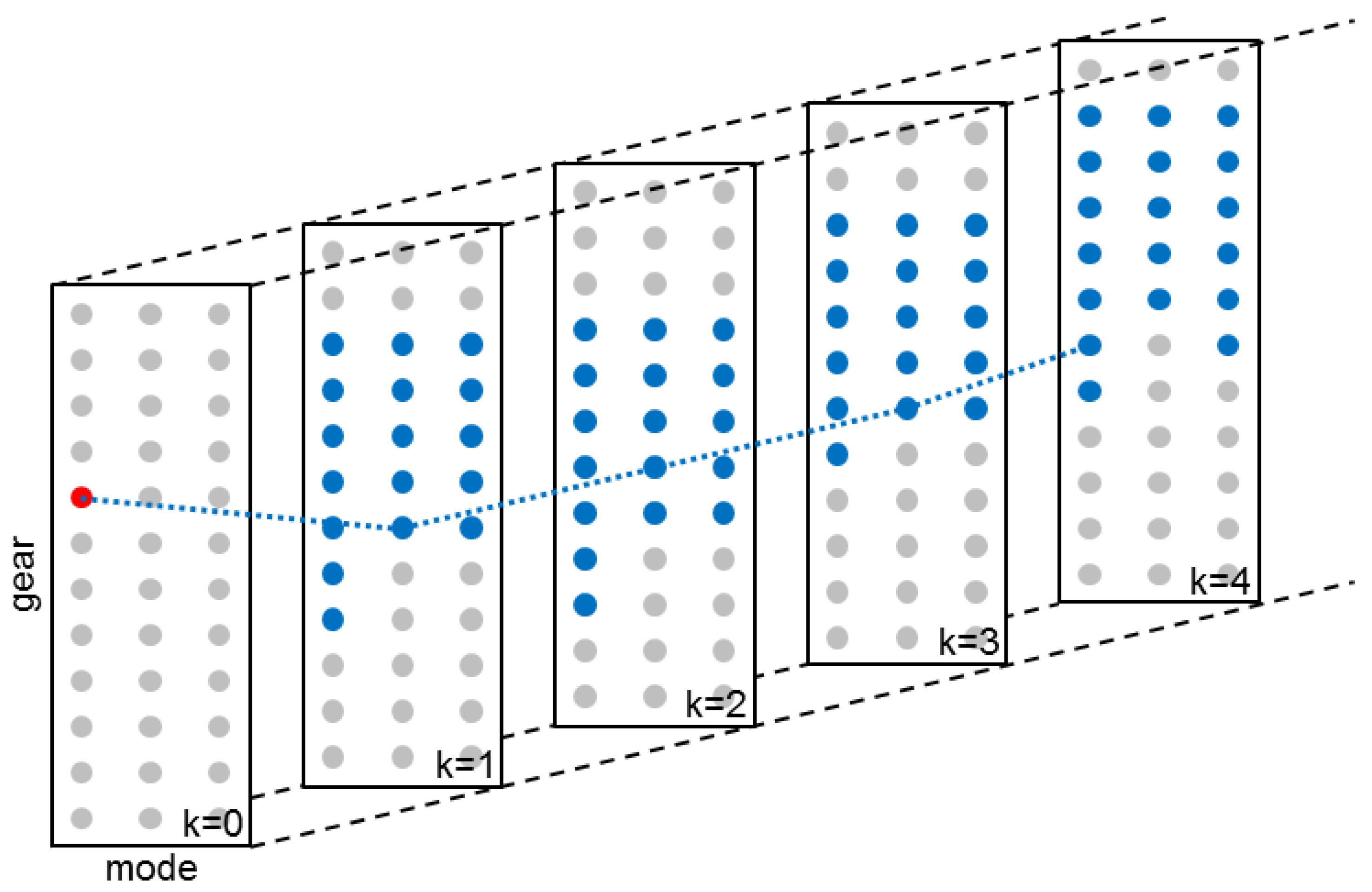
Figure 11.
For dealing with constraints, non-unique solutions and a limited horizon, the flowchart shows the procedure for solving the boundary value problems (BVP). Starting with one unsolved (sub)problem (SP), from to , the process is started. Dependent on the number of constraint violations, the procedure ends with a set of solved subproblems, each providing a segment of over the complete horizon. Each subproblem contains the solution to a BVP, and dependent on the stated conditions, the additional procedures I1, I2 or I3 are needed.
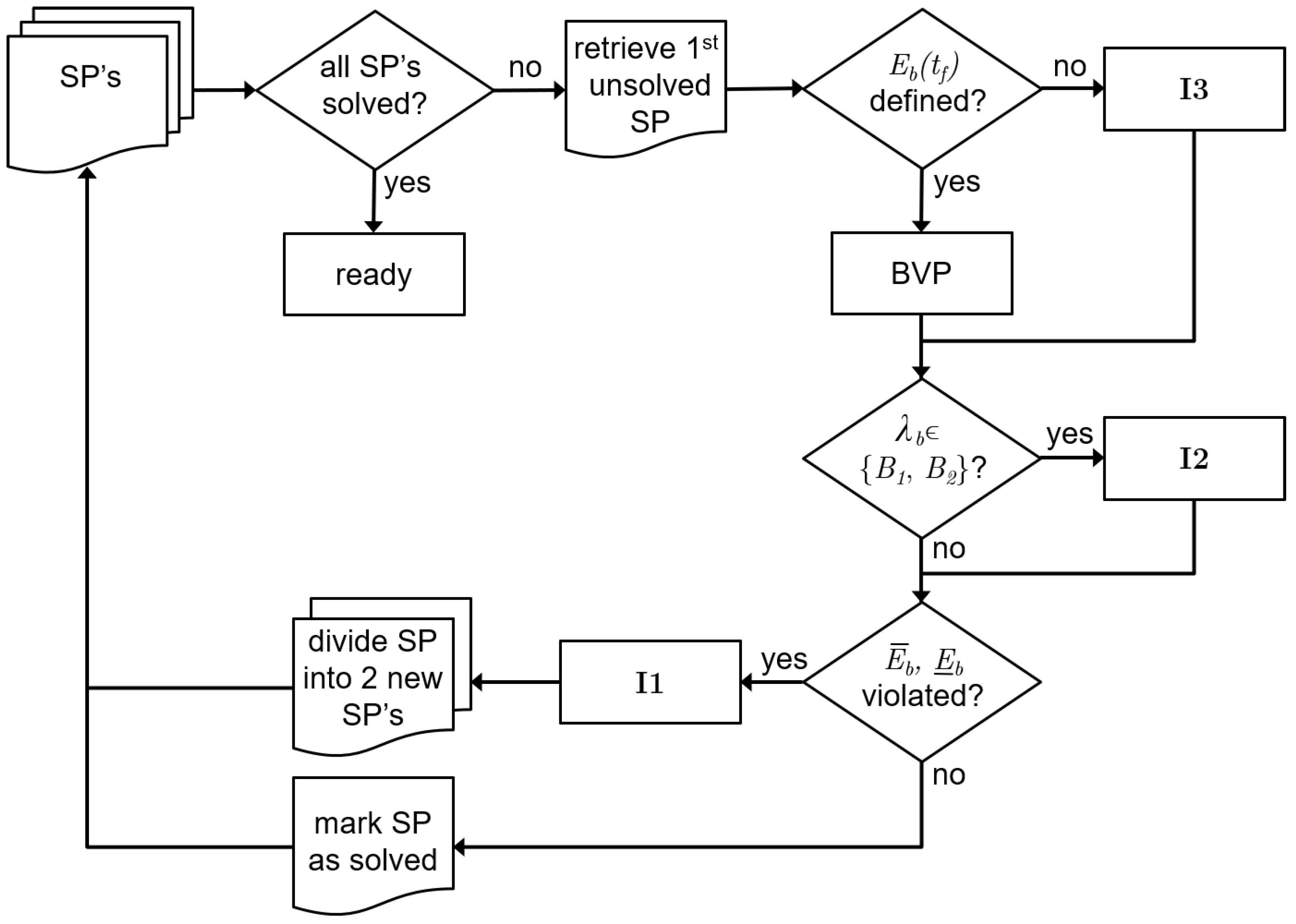
Figure 12.
Changing the constant for a drive cycle, causes jumps in the charge sustenance, due to non-unique (singular) solutions at and .
Figure 12.
Changing the constant for a drive cycle, causes jumps in the charge sustenance, due to non-unique (singular) solutions at and .

Figure 13.
Illustration of algorithm I2a. Power demand of a drive segment with and two optimal modes: ( is positive during high power demands, resulting in too low ) and ( is zero during high power demands, resulting in too high ). A charge sustaining trajectory (), is possible with one switch at or , or with infinitely many switchings indicated as .

Figure 14.
Illustration of algorithm I2b, first part. Starting with the lower boundary is violated at and a switch must be made to . However, s as switching point is too late, as exceeds with .
Figure 14.
Illustration of algorithm I2b, first part. Starting with the lower boundary is violated at and a switch must be made to . However, s as switching point is too late, as exceeds with .
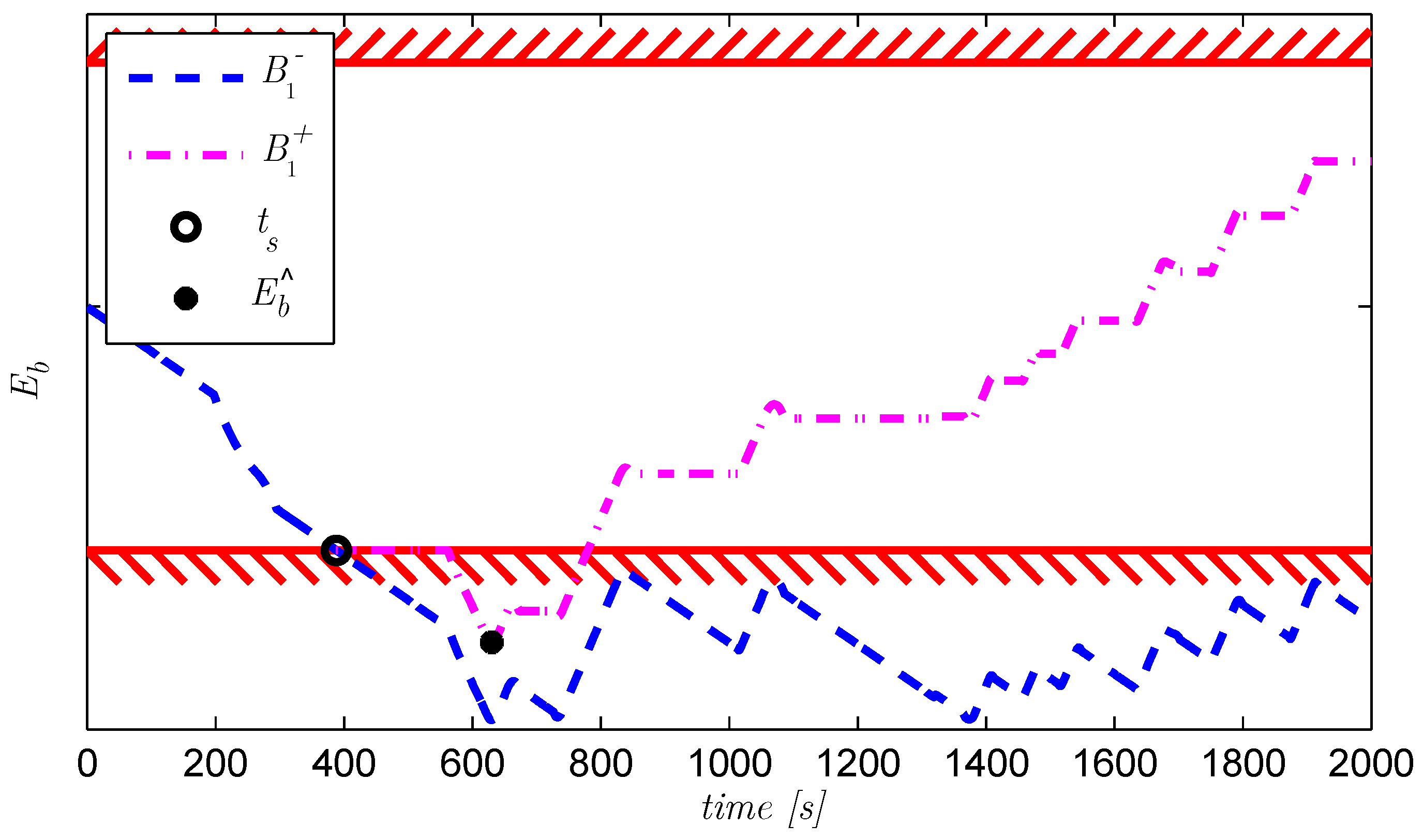
Figure 15.
Illustration of algorithm I2b, second part. A new s is found, and is continued, until at s the switch to has to be made to ensure .
Figure 15.
Illustration of algorithm I2b, second part. A new s is found, and is continued, until at s the switch to has to be made to ensure .

Figure 16.
Elevation profile of the short test cycle.

Figure 17.
High fidelity simulation results on a representative long-haul cycle. The previewing Energy Management System (EMS) saves an additional fuel to the baseline EMS.
Figure 17.
High fidelity simulation results on a representative long-haul cycle. The previewing Energy Management System (EMS) saves an additional fuel to the baseline EMS.

Table 1.
Optimizing Energy Management System (EMS) algorithms, for power-split, stop-start and gear. ‘Cost’ indicates if switching events are penalized in the algorithm. See Table 2 for the used abbreviations.
Table 1.
Optimizing Energy Management System (EMS) algorithms, for power-split, stop-start and gear. ‘Cost’ indicates if switching events are penalized in the algorithm. See Table 2 for the used abbreviations.
| Reference | Power-Split | Stop-Start | Gear Selection |
|---|---|---|---|
| [15] | PMP | PMP | - |
| [16] | QP | RB | - |
| [17] | QP | PMP | RB |
| [18] | PMP | DP | DP |
| [19] | QP | DP + cost | DP + cost |
| [20] | MILP | MILP + cost | MILP + cost |
| this work | PMP | DP + cost | DP + cost |
Table 2.
Abbreviations.
| Components | |
| BT | Battery |
| CE | Combustion Engine |
| CL | Clutch |
| EMS | Energy Management System |
| FT | Fuel Tank |
| GB | Gearbox |
| HEV | Hybrid Electric Vehicle |
| MG | Motor Generator |
| RD | Road |
| VH | Vehicle |
| Algorithms | |
| DP | Dynamic Program |
| MILP | Mixed Integer Linear Program |
| PMP | Pontryagin’s Minimum Principle |
| QP | Quadratic Program |
| RB | Rule Based (heuristics) |
Table 3.
Model parameters for the internal combustion engine (CE), motor generator (MG), battery (BT) and vehicle (VH).
Table 3.
Model parameters for the internal combustion engine (CE), motor generator (MG), battery (BT) and vehicle (VH).
| Model | Parameter | Value | Unit | Description |
|---|---|---|---|---|
| CE | 0.45 | - | indicated efficiency | |
| W | friction (cf. Figure 3) | |||
| W | minimum power (cf. Figure 3) | |||
| W | maximum power (cf. Figure 3) | |||
| 3 | kg m | moment of inertia | ||
| MG | 0.95 | - | mechanical efficiency | |
| W | friction (cf. Figure 3) | |||
| W | minimum power (cf. Figure 3) | |||
| W | maximum power (cf. Figure 3) | |||
| 1.5 | kg m | moment of inertia | ||
| BT | 1/W | loss coefficient | ||
| J | effective battery size | |||
| VH | m | kg | vehicle mass | |
| 1.2 | kg/m | air density | ||
| 0.65 | - | air drag coefficient | ||
| A | 10 | m | frontal area | |
| - | rolling resistance coefficient | |||
| 52.2 | - | drive ratio | ||
| 1.29 | - | gear base constant | ||
| g | 9.8 | m/s | gravitational constant |
Table 4.
Driveline modes M.
| M | Description | CL | CL | ||
|---|---|---|---|---|---|
| combined | closed | closed | = = | ||
| engine-only | closed | open | = = 0 | ||
| motor-only | open | closed | = = 0 | ||
| open driveline | open | open | = = 0 | 0 |
Table 5.
Generic optimization problem, subdivided into three levels (i).
| ‘Generic’ | ‘Velocity’ | ‘Battery Energy’ | ‘Power-Split’ | |
|---|---|---|---|---|
| 3 | 2 | 1 | ||
| 0 | 0 | |||
| 0 | ||||
Table 6.
Explicit solution of the power-split as a function of the mode.
| Mode | Description | |
|---|---|---|
| motor-only | ||
| engine-only | 0 | |
| combined |
Table 7.
Energy consumption over the short test cycle. MPC: model predictive controller.
| J [MJ] | Energy Reduction [%] | |
|---|---|---|
| non-hybrid | 16.8 | 0 |
| iteration 0 | 7.91 | 52.9 |
| iteration 1 | 7.90 | 53.0 |
| MPC | 7.93 | 52.8 |
Table 8.
Fuel savings on a typical long-haul route. EMS: energy management system.
| Vehicle | Fuel [l/100 km] | Fuel [%] |
|---|---|---|
| non-hybrid | 33.0 | 0 |
| EMS ‘baseline’ | 31.1 | −5.8 |
| EMS ‘preview’ | 30.7 | −7.0 |
© 2019 by the authors. Licensee MDPI, Basel, Switzerland. This article is an open access article distributed under the terms and conditions of the Creative Commons Attribution (CC BY) license (http://creativecommons.org/licenses/by/4.0/).
Share and Cite
MDPI and ACS Style
van Reeven, V.; Hofman, T. Multi-Level Energy Management for Hybrid Electric Vehicles—Part I. Vehicles 2019, 1, 3-40. https://doi.org/10.3390/vehicles1010002
AMA Style
van Reeven V, Hofman T. Multi-Level Energy Management for Hybrid Electric Vehicles—Part I. Vehicles. 2019; 1(1):3-40. https://doi.org/10.3390/vehicles1010002
Chicago/Turabian Stylevan Reeven, Vital, and Theo Hofman. 2019. "Multi-Level Energy Management for Hybrid Electric Vehicles—Part I" Vehicles 1, no. 1: 3-40. https://doi.org/10.3390/vehicles1010002