Tutorial on the Use of the regsem Package in R

Abstract

Sparse estimation through regularization is gaining popularity in psychological research. Such techniques penalize the complexity of the model and could perform variable/path selection in an automatic way, and thus are particularly useful in models that have small parameter-to-sample-size ratios. This paper gives a detailed tutorial of the R package regsem, which implements regularization for structural equation models. Example R code is also provided to highlight the key arguments of implementing regularized structural equation models in this package. The tutorial ends by discussing remedies of some known drawbacks of a popular type of regularization, computational methods supported by the package that can improve the selection result, and some other practical issues such as dealing with missing data and categorical variables.

1. Introduction

With the ability to assess relationships between latent constructs and observed variables, structural equation modeling (SEM) has become an increasingly popular choice for psychological researchers due to its flexibility as a general modeling framework. Given that it is often easier to collect more variables than participants, researchers increasingly aim to estimate large models with limited numbers of participants. However, this practice would deteriorate the trustworthiness of the results given violations of recommended observations to estimated parameters (N/q) ratios. For instance, Kline [1] recommended 20 observations (participants) for each estimated parameter in the model. Alternatively, when the data are perfectly well-behaved (i.e., normally distributed, no missing data or outlying cases, etc.), Bentler and Chou [2] have suggested this ratio can go as low as five to one.

Besides obtaining more respondents, reducing the number of parameters estimated is another option. Although specifying a model smaller than the “true” model may bias the parameter estimates, this reduced model may work better for estimation from a bias–variance tradeoff perspective. Regularization is one such method to accomplish this, performing variable/path selection by penalizing the complexity (number of parameters estimated) of the model, and thus producing a more parsimonious model. It has been successfully applied in many areas such as regression and graphical modeling, and has been introduced to SEM more recently (e.g., regularized SEM and penalized likelihood SEM) [3,4].

1.1. Regularized Regression

When the assumptions required by ordinary least squares (OLS) regression are met, OLS produces the best linear unbiased estimator (with lowest variance). However, as the number of features grows, the OLS assumptions would typically break down and the models could overfit the training sample, causing the out-of-sample error to increase. Regularization methods discourage complex models by penalizing the magnitude of the coefficients so that the coefficients will be shrunken towards zero, thereby reducing the size and fluctuations of the coefficients as well as reducing the variance of the models. The two most commonly used forms of regularization in regression are the ridge [5], which constrains the coefficients by the $L_2$ norm, and the least absolute shrinkage and selection operator (lasso) [6], which utilizes the $L_1$ norm. Given the outcome vector $y$ and predictor matrix $X=\left(x_{ij}\right)\in {ℝ}^{n\times p}$, the estimates of ridge and lasso are defined as:

$${\widehat{\beta }}^{ridge}=argmin \{{\displaystyle \sum }_{i=1}^N{\left(yi-{\beta }_0-{{\displaystyle \sum }}_{j=1}^p{x}_{ij}{\beta }_j\right)}^2+\lambda {{\displaystyle \sum }}_{j=i}^p{\beta }_j^2\}$$

(1)

$${\widehat{\beta }}^{lasso}=argmin \{{\displaystyle \sum }_{i=1}^N{\left(yi-{\beta }_0-{{\displaystyle \sum }}_{j=1}^p{x}_{ij}{\beta }_j\right)}^2+\lambda {{\displaystyle \sum }}_{j=i}^p\left|{\beta }_j\right|\}$$

(2)

with ${\beta }_0$ being the intercept, ${\beta }_j$ being the coefficient for $x_j$, and $\lambda$ being a tuning parameter controlling the amount of shrinkage. As $\lambda$ increases, the $\beta$ estimates are shrunken towards 0, and the estimates are equivalent to OLS regression when $\lambda =0$. The optimal value of $\lambda$ is usually determined by cross-validation. The $L_2$ penalty used in ridge regression helps to reduce the model complexity and multi-collinearity, whereas the $L_1$ penalty used by lasso can further lead the parameters to zero, and thus not only helps in reducing over-fitting, but also can perform feature selection.

There are various alternative forms of regularization that can be seen as subsets or generalizations of these two procedures; for example, the elastic net [7], which is a linear combination of the ridge and the lasso with an additional tuning parameter $\alpha$ is defined as:

$${\widehat{\beta }}^{enet}=argmin\{{\displaystyle \sum }_{i=1}^N{\left(yi-{\beta }_0-{{\displaystyle \sum }}_{j=1}^p{x}_{ij}{\beta }_j\right)}^2+\lambda ((1-\alpha ){{\displaystyle \sum }}_{j=i}^p{\beta }_j^2+\alpha {{\displaystyle \sum }}_{j=i}^p\left|{\beta }_j\right|)\}$$

(3)

By incorporating both ridge and lasso penalties, the elastic net integrates the positives of both, handling collinearity and performing variable selection. Particularly when predictors are moderately correlated, the elastic net will often outperform the lasso for variable selection [7].

1.2. Regularized SEM

Similar to regularized regression, a penalty term is added to the traditional maximum likelihood estimation (MLE) fit function in regularized SEM as follows:

$$F_{regsem}\left(\theta \right)=\underset{F_{MLE}}{\underbrace{\begin{array}{c}\log \left(\left|\Sigma \left(\theta \right)\right|\right)+tr\left(C*{\Sigma }^{-1}\left(\theta \right)\right)-\log \left(\left|C\right|\right)-p\\ +{\left(m-\mu \left(\theta \right)\right)}^{’}{\Sigma }^{-1}\left(\theta \right)\left(m-\mu \left(\theta \right)\right)\end{array}}}+\underset{penalty}{\underbrace{\lambda P\left(\cdot \right) }}$$

(4)

where $\theta$ is the set of parameters estimated, $\mu \left(\theta \right)$ and $\Sigma \left(\theta \right)$ are the model implied mean and covariance matrices, respectively, $m$ and $C$ are the observed mean and covariance matrices, and $p$ is the number of variables. The regularization parameter $\lambda$ is a tuning parameter that quantifies the influence of the penalty. The larger λ corresponds to a larger penalty, and thus would result in greater shrinkage of the coefficient sizes. For regularized SEM, its optimal value is often determined through cross-validation or based on information criteria, such as Akaike information criterion (AIC) [8] and Bayesian information criterion (BIC) [9]. Prior research shows that the BIC generally performs well in practice for selecting λ that results in reasonable parameter estimates for regularized factor analysis models [3,10]. $P\left(\cdot \right)$ is a general penalty function which reflects the sum of all selected coefficients, and can take different forms like the lasso ($L_1$ norm ${\parallel \cdot \parallel }_1$), ridge ($L_2$ norm ${\parallel \cdot \parallel }_2$), and elastic net ($\left(1-\alpha \right){\parallel \cdot \parallel }_1+\alpha {\parallel \cdot \parallel }_2$) just as with regularized regression. With the penalty term added, the new fit function would yield a different set of parameter estimates, which are biased towards zero. When the “summing” technique is carefully chosen (e.g., $L_1$ norm in the case of lasso), some of the less relevant parameters are forced to zero, thus performing variable selection, or creating a simpler model structure. From a bias–variance perspective, such methods trade off an increase in bias with a decrease in variance, and thus could potentially produce lower total generalization error. For an overview, see Yarkoni and Westfall [11].

Different penalties do affect the selection result. For example, the lasso, possibly the most popular choice of penalty, is only consistent for variable selection under certain restricted conditions (oracle property) [12,13]. It also has problems such as tending to select one variable from a group of highly correlated variables and ignoring the others [7], and high false positive rates. Many other extensions are thus proposed to overcome these limitations, among which the smoothly clipped absolute deviation (SCAD) [14] and the minimax concave penalty (MCP) [15] are the two most well-known penalties. Compared to the lasso, both the SCAD and MCP penalize large parameters less, while applying similar amounts of shrinkage to the lasso for small parameters. Theoretical results in the GLM family indicate that SCAD and MCP can both yield oracle estimators [14,15,16]. It has also been shown that they outperform lasso, and will select the true model with high probability asymptotically in regularized SEM [4], and penalized likelihood EFA [17] through simulation studies.

The application of regularized SEM falls between confirmatory modeling, where the hypothesized model is constructed based on theory and/or previous research, and exploratory modeling, where no a priori hypotheses about latent factor composition or patterns of the measured variables are made. Researchers could place penalties only on those uncertain parts of the model, while not penalizing the parts of the model that have theoretical backing. This can take many forms, including and not limited to selecting among multiple predictors of a latent variable [18], simplifying factor structure by removing cross-loadings [19], and determining whether additional linear terms are necessary in longitudinal models, among many others.

In this paper, we wish to provide a detailed tutorial on performing regularization in SEM using the R package regsem [20].

2. Implementation

Regularized SEM is implemented in the R statistical environment using the regsem package. The model syntax follows the R package lavaan [21], which is a general and widely used SEM software program that can fit a wide range of models with various estimation methods. The main functions of the regsem package are regsem(), multi_optim(), and cv_regsem(). Those functions take in a model object fitted in lavaan (i.e., output of function lavaan(), sem(), cfa(), or growth()), specify parameters to penalize, the type of penalty [22], as well as the penalty values, then translate the model object into Reticular Action Model (RAM) [23,24] notation to derive the model implied covariance matrix with the specified parameters penalized. The differences of the three main functions lie in the number of penalty levels and starting values considered. The regsem() and the multi_optim() functions take only one penalty value, with the multi_optim() function further allowing the use of multiple random starting values for models that have difficulty converging. On the other hand, the cv_regsem() function runs regularization across a set of varying penalty values. Paired with the use of an information criterion, the cv_regsem() function is able to select a final model with, comparatively, the best penalty value.

3. Empirical Example

We now give an example of implementing the regsem package to further discuss the details. Here, we use an integrated dataset consisting of five publicly available datasets: National Comorbidity Survey—Baseline (NCS) [25]; NCS—Replication [26]; National Survey of American Life (NSAL) [26]; National Survey of American Life—Adolescent Supplement [27]; and the National Latino and Asian American Study [26]. Each survey was designed to study the prevalence and correlates of psychological disorders among individuals living in the United States. Combined, 25,159 respondents were surveyed; however, response rates on individual items within and across datasets vary. For demonstration purposes, we randomly selected a sample of 1000 to mimic a limited sample size situation when regularization is desired. For this example, we selected 18 items (11 assessed within four datasets; 7 assessed within five datasets) that assessed the presence of symptom-level information (i.e., felt depressed most days, has a limited appetite most days, was so restless that others noticed) as it occurred during an individual’s most severe depressive episode.

Given that this analysis is a part of a larger study, our motivation was to combine depression items from across multiple scales, assessed across the five datasets, to identify an optimal factor structure to be used in additional analyses. Our eventual goal was an adequately fitting CFA model, as we desired some degree of clarity regarding the interpretation of each factor. However, given that we did not have an a priori model, we started with EFA to derive the number of factors.

We store the data to object dat.sub2. The path diagram of the constructed model is displayed in Figure 1.

Before fitting the model in regsem, we need to organize our data. There are two major points here. The first is to transfer the data type of the endogenous variables of the model to continuous. This is because the regsem package works with the maximum likelihood discrepancy function, which assumes that the endogenous variables are continuous and normally distributed. With this, even though there are available options in lavaan that accommodate categorical variables, those options are not currently supported by regsem. For more discussion on categorical variables, see Section 4.5.

The second point is with respect to the scale of the variables. In regularized regression, it is suggested to standardize the variables before fitting the model. This is because the effect of the regularization is not orthogonal to the scales of the variables. For penalty types such as ridge and lasso, larger coefficients are penalized more, which will make the regularization biased and tend to penalize features with smaller scales. For SEM, the covariance matrix becomes the correlation matrix after standardizing all of the variables. This will not create a problem for maximum likelihood without the penalty, since the results based on covariance and correlation are essentially equivalent except for the scale. However, this invariance property of maximum likelihood no longer holds after the penalty is added; that is, results based on covariance and correlation are not equivalent for regularized SEM. Huang et al. [4] thus suggest fixing the scaling loadings deliberately, such that all of the latent variables have variances of around one. Jin et al. [17] suggest working with the correlation matrix, then transferring back to the covariance scale in their study of penalized likelihood EFA. We recommend standardizing only the variables which have at least one path to be penalized before fitting the regularized SEM model to eliminate the effect of the scale on variable/path selection. A second step of fitting the restricted model after the selection (“relaxed lasso”) [28] could then be done on the original scale. We suggest that researchers transform the variable scale carefully based on the research question before the analysis.

To evaluate the factor structure, we first used parallel analysis to identify an appropriate number of factors, of which five seemed the most appropriate. From this, we followed the procedure of Scharf and Nestler [19] and specified an EFA model, with each factor loading penalized. This initial model is not identified; however, as the penalties increase, the degrees of freedom will become positive as additional factor loadings are set to zero. In

Table 1. R code for constructing the model and organizing data.

R Code 1

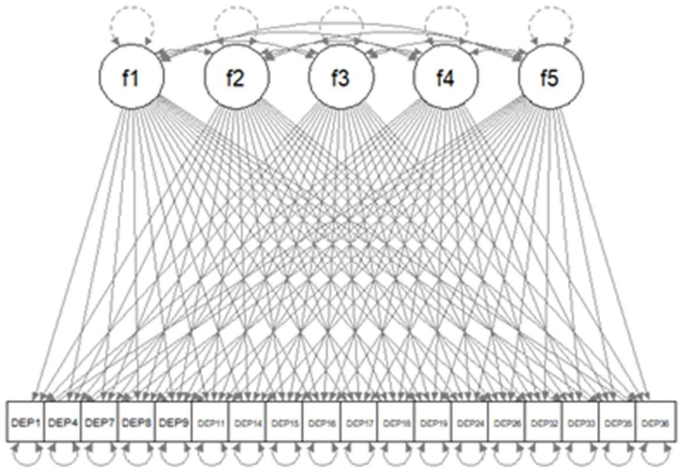
library(lavaan) lav.mod<-paste( “f1=~NA*”,paste(colnames(dat.sub2),collapse=“+”),”\n”, “f2=~NA*”,paste(colnames(dat.sub2),collapse=“+”),”\n”, “f3=~NA*”,paste(colnames(dat.sub2),collapse=“+”),”\n”, “f4=~NA*”,paste(colnames(dat.sub2),collapse=“+”),”\n”, “f5=~NA*”,paste(colnames(dat.sub2),collapse=“+”),”\n”, “f1~~1*f1; f2~~1*f2; f3~~1*f3; f4~~1*f4; f5~~1*f5”) dat.s<-scale(dat.sub2) lav.out<-cfa(dat.s,model=lav.mod,missing=“listwise”)

¹ We standardize all variables here since each of them has at least one path to be penalized in this example. In other models, researchers should not standardize variables with no related path to be penalized.

, we show the R code for constructing the model and organizing the example data.

For the model fitted in lavaan, any wrapper function can be used. lavaan by default sets estimator = “ML”. Researchers should not change this default, as the other options are not currently supported by regsem. When there is missing data, regsem currently supports listwise deletion and full information maximum likelihood (FIML). Since lavaan and regsem both use listwise deletion by default, we demonstrate only the use of listwise deletion for our example here. The FIML option and other options related to missing data will be further discussed in the Discussion section. Here, our model fitted by lavaan is not identified. This will not create a problem for regsem, since regsem() uses the lavaan object only to extract the sample covariance matrix and other aspects of the data. One can also specify do.fit=FALSE in this step. The model will become identified through path/variable selection. For an example of using regsem to identify EFA models, see [23,24].

After running a model in lavaan, we can then add penalties to the uncertain structural coefficients in regsem. There are multiple ways to specify this in the pars_pen argument. By default, regsem penalizes all regression parameters (pars_pen = “regression”). One can also specify all loadings (pars_pen = “loadings”), or both (pars_pen = c(“regressions”, “loadings”)). Since regularized SEM is semi-confirmatory, researchers may want to leave the theory-based part of the model unpenalized. Though those unpenalized parameters are estimated along with penalized ones, they should not be included in the pars_pen argument. If parameter labels are used in the lavaan model specification, those labels of the parameters to be penalized can be directly passed to the pars_pen argument. Otherwise, one can find the corresponding parameter numbers by looking at the output of the extractMatrices() function. An example of the R code and output is shown in

Table 2. R code and output for extracting the RAM matrices and determining the numbering of parameters to be penalized.

R code
library(regsem) A<-extractMatrices(lav.out)$A head(A[1:18,19:23])
Output 1
f1 f2 f3 f4 f5 DEP1  1 19 37 55 73 DEP4  2 20 38 56 74 DEP7  3 21 39 57 75 DEP8  4 22 40 58 76 DEP9  5 23 41 59 77 DEP11 6 24 42 60 78

¹ We only demonstrate the first 6 rows of the block of matrix A that corresponds to the parameter numbers of the cross-loadings.

.

The package regsem is built upon RAM notation [23,24]. The extractMatrices() function extracts and returns the RAM matrices of the SEM model estimated in lavaan. The filter matrix F ($F) indicates which variables are observed (as opposed to latent), the asymmetric matrix A ($A_est) stores the estimated direct path coefficients, and the symmetric matrix S ($S_est) stores the estimated variances and covariances. Those matrices are then used to derive the implied covariance matrix of the model. The $A matrix and $S matrix in the extractMatrices() output store the corresponding parameter number of each estimated parameter. We can refer to those matrices and then pass the desired parameter numbers to the pars_pen argument. For more detail on RAM notation and its application to regsem, see Jacobucci et al. [3]. In our example, we would like to penalize all paths with loadings smaller than 0.5 from the rotated EFA model. We deviate from the Scharf and Nestler [19] procedure in this regard, as in our experience, allowing large factor loadings to go unpenalized assists in achieving a converged solution as fewer constraints are being placed on the model. The corresponding parameters penalized are summarized in

Table 3. Parameter to be penalized.

R code
pars.pen <- A[1:18,19:23][load.2<.5] pars.pen
Output
[1] 1 2 3 6 7 8 9 10 11 12 13 14 15 16 17 18 20 22 23 26 [21] 27 28 29 30 31 32 33 34 37 38 39 40 41 42 43 45 46 49 50 51 [41] 52 53 54 55 56 57 58 59 60 61 62 65 66 67 68 69 70 71 72 73 [61] 75 76 77 78 79 80 81 82 83 84 85 89 90

.

We can then set the penalty type (e.g., type = “lasso”), the number of penalty values we want to test (e.g., n.lambda = 20), and how much the penalty should increase (e.g., jump = 0.05). The latter two arguments may vary for different models and data, as the impact of the penalty depends on the scale of $F_{MLE}$. We suggest including a wider range of penalties initially, as regsem will terminate when testing higher penalty values if all parameters have been set to zero. One can also determine the penalty range by looking at the parameter trajectories, which is the trajectory of the value of each penalized parameter at different penalty levels. One can further visualize the chosen “optimal” penalty level by specifying show.minimum argument equal to the desired criteria for optimality (detailed later). The parameter trajectories corresponding to our example are shown in Figure 2. At penalty 0.02, the model becomes identified, and the optimal penalty is 0.16 as shown in this plot.

For cv_regsem() to examine the penalties and select the best model, a fit index needs to be specified as well. As the penalty increases, some parameters would be set to 0, making $F_{ML}$ larger (worse). However, the degrees of freedom would increase as well. Further, we can see in

Table 4. R code for lasso regularization and corresponding output.

R code 1
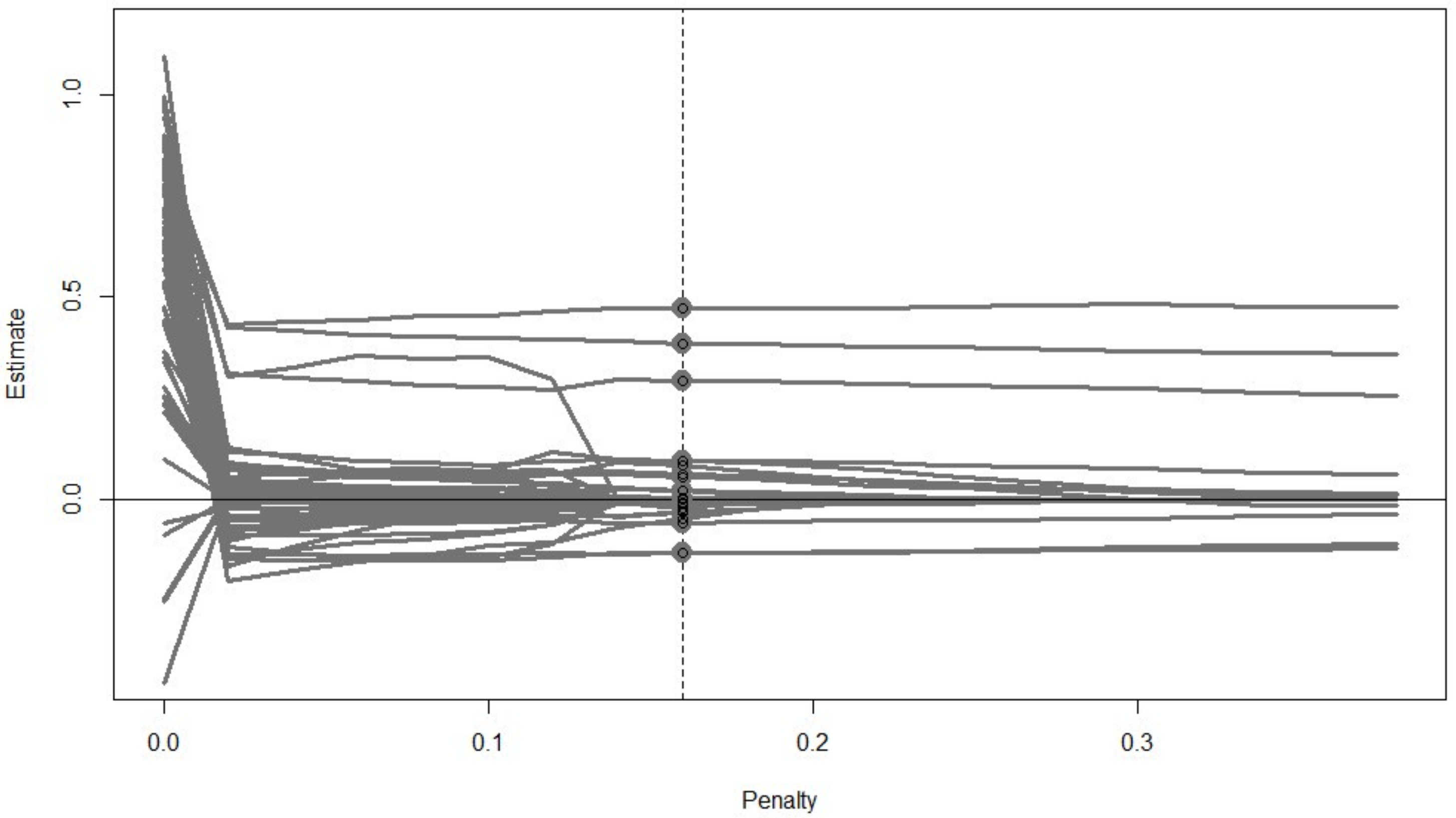
out.reg<-cv_regsem(lav.out, type = “lasso”, pars_pen = pars.pen, n.lambda = 20, jump = 0.02) out.reg plot(out.reg, show.minimum=“BIC”)
Output 2,3
out.reg$parameters
	f1 -> DEP1		f1 -> DEP4	f1 -> DEP7	f1 -> DEP8
[1,]	0.816		0.675	0.869	0.012
[2,]	−0.004		0.000	0.425	−0.557
[3,]	−0.005		0.000	0.416	−0.554
[4,]	−0.004		0.000	0.407	−0.550
[5,]	−0.004		0.000	0.403	−0.550
[6,]	−0.002		0.000	0.398	−0.548
...
out.reg$fits
	lambda	conv	rmsea	BIC	chisq
[1,]	0.00	0	0.12929	22002.41	6.828856e+02
[2,]	0.02	0	0.10402	21835.50	6.867450e+02
...
[9,]	0.16	0	0.09721	21787.29	8.027334e+02
...
[11,]	0.20	1	0.00000	−14315219.42	−1.433654e+07
[12,]	0.22	0	0.09851	21810.05	8.451946e+02
...
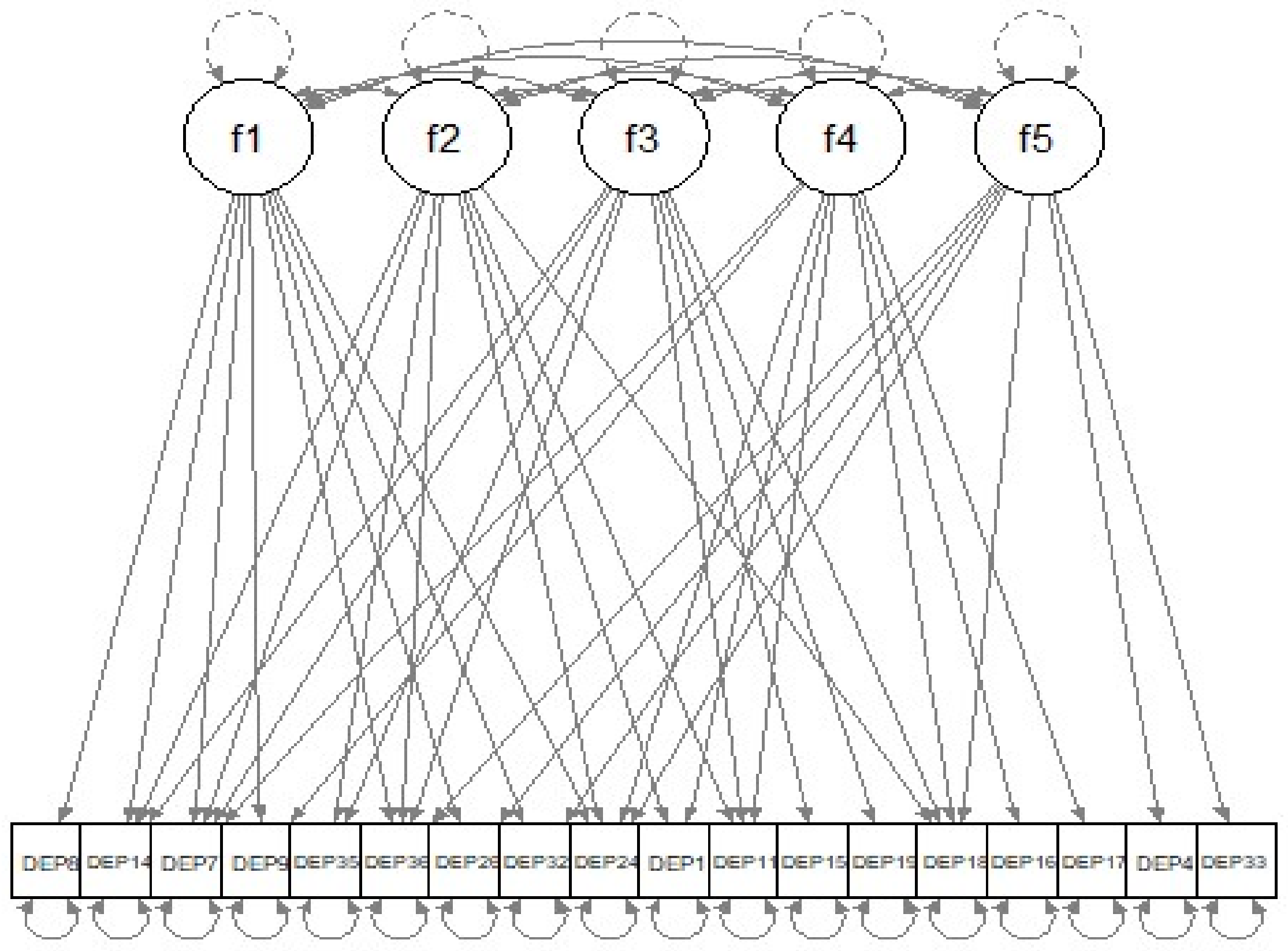
out.reg$final_pars
f1 -> DEP1		f1 -> DEP4		f1 -> DEP7	f1 -> DEP8
0.000		0.000		0.384	−0.548
f1 -> DEP9		f1 -> DEP11		f1 -> DEP14	f1 -> DEP15
−0.902		0.000		−0.009	0.000
f1 -> DEP16		f1 -> DEP17		f1 -> DEP18	f1 -> DEP19
0.000		0.000		0.000	0.000
f1 -> DEP24		f1 -> DEP26		f1 -> DEP32	f1 -> DEP33
−0.058		0.002		-0.010	0.000
f1 -> DEP35		f1 -> DEP36		...
0.000		0.023

¹ This plot gives the parameter trajectories shown in Figure 2. ² We only display part of the output for the model. There are other outputs that we do not display here (such as $pars_pen, $df (degrees of freedom at each penalty level), and $metric, etc.). Please refer to the Supplementary Materials for complete results. ³ Note in $parameters that the parameter estimates are highly variable at the displayed penalty values as the model is still unidentified.

a large change in the parameter estimates from lambda = 0 to lambda = 0.02. This is caused by an unpenalized model being unidentified, as there are more parameters than cells in the covariance matrix. By adding even a small penalty, the dimensionality of the model is reduced, thus resulting in more stable parameter estimates. This can further be seen in Figure 2.

The regsem package, by default, uses the Bayesian Information Criteria (BIC) [9] to select a final model, which takes both the likelihood and degrees of freedom into account, and thus still could improve (decrease) as penalty increases. The final model is selected to be the one that corresponds to the lowest BIC value of all models that converged. To compare the selection performance of other information criteria, see Jacobucci et al. [3] and Lüdtke et al. [29]. The output of our example model is shown in

Table 5. R code and output for using multi_optim() function for non-convergence cases.

R code
out.20 <- multi_optim(lav.out, type = “lasso”, pars_pen = pars.pen, lambda = 0.20) summary(out.20)
Output1
Out.20$returnVals
convergence	df	fit	rmsea	BIC
0	92	0.7426382	0.12149	22120.89

¹ There are other outputs that we do not display here.

.

The output of cv_regsem() contains the parameter estimates of the models fitted at each penalty level in $parameters, their corresponding model fit information in $fits, and the parameter estimates of the best-fitted model according to the chosen fit index metric (here, BIC) in $final_pars. Note that this best-fitted model is only considering models that converged (“conv” = 0 in $fits means converged, whereas “conv” = 1 means non-convergence). In our example, the model did not converge with several penalty levels (e.g., when lambda = 0.20). One can choose to explore each penalty value further by testing multiple starting values using the multi_optim() function, or this can be done automatically in cv_regsem() by setting multi.iter = TRUE. The demonstration R code for the case lambda = 0.20 and the corresponding output is shown in Table 5. The BIC value of the model at this penalty level is 22,120.89, which is larger than the BIC value of 21,787.29 at lambda = 0.16. Thus, the optimal model is still the one with penalty level equal to 0.16.

In $final_pars of the cv_regsem() output, we can see that several parameters (for example, the ones corresponding to path “f1 -> DEP1” and path “f1 -> DEP4”, etc.) now have parameter estimates of zero. Those are the paths to be removed from the current model. We recommend the use of the two-step “relaxed” lasso [25]; that is, to refit the model with those paths removed. For this example, 51 paths are removed based on the selection result. The path diagram of the reduced model is displayed in Figure 3. Ideally, one should evaluate this simplified model on a new set of data. Here, we demonstrate this on another random sample of 1000 from our dataset. The fitted model has a CFI of 0.946, a TLI of 0.920, and an RMSEA of 0.095 (90% CI (0.089, 0.101)).

Given that we now have a final CFA model derived from the use of lasso penalties, each factor with only a handful of loadings, we can interpret the meaning of the resultant factors. For example, factor one predominantly includes depression items related to change in appetite and weight; factor two items pertain to symptoms of low energy; factor three relates to symptoms that assess energy levels more broadly, rather than just low energy; factor four items map on to behavioral changes associated with depression, such as appetite, weight, sleep, and talkativeness; and factor five most represents emotional distress, such as crying, feeling worthless, and suicidal thinking. However, it is important to note that there are significant item cross-loadings, suggesting multiple factors have significant conceptual overlap, as demonstrated by the fact that four of the assessed symptoms load onto four of the five factors. Thus, we are not advocating for this to be a solution for researchers moving forward, but rather a conceptual demonstration.

4. Extensions

4.1. Other Application Scenarios

The application of regularized SEM is not limited to the model we demonstrated in this tutorial, but the main steps and codes are the same. In this subsection, we outline a subset of the scenarios suitable for applying the regsem package.

4.1.1. Regression/Path Analysis Models

Regularization is a widely adopted method in regression. Since SEM can be seen as a generalization of regression models, regsem can also be applied to regression models as a substitute for a more commonly used R package for applying regularized regression models, which is glmnet. Besides regression, other path analysis models could also be specified in the SEM framework, and thus could be explored through regsem in semi-confirmatory settings. For example, Serang et al. [30] have proposed exploratory mediation analysis via regularization (XMed) which can be performed using the regsem package.

4.1.2. Factor Analysis Models

Scharf and Nestler [19] have applied regsem for exploratory factor analysis and found that both rotated and regularized EFA tended to underestimate cross-loadings and inflate factor correlations when the factor structures are complex, while regularized EFA was able to recover loading patterns as long as some of the items followed a simple structure. They thus conclude that regularization is a suitable alternative to factor rotation for psychometric applications. Huang [31] used regularized SEM to simplify factor structure by removing cross-loadings for the big five personality traits for the bfi data from the R package psych [32]. The performance of extensions of regularized SEM for removing cross-loadings is also studied by Li and Jacobucci [33] through a simulation study.

4.1.3. Longitudinal Models

Although a number of statistical frameworks are available for analysis with longitudinal data, the use of structural equation modeling has become increasingly popular. Jacobucci and Grimm [34] introduce multiple ways for regularization to be used with the latent change scores (LCS) model. They showed that using both frequentist and Bayesian regularization allowed for a simplified process in choosing the best model, while also increasing the flexibility of the LCS model to incorporate additional parameterizations across both univariate and bivariate LCS models. Further, SEM is being increasingly applied to intensive longitudinal datasets, which can often contain a large number of both undirected and directed paths. Within this, lasso penalties have been applied to “discover” the optimal configuration of paths within hybrid vector autoregression models [35].

4.1.4. Group-Based SEM

Besides applying regularization methods for single-group analysis, methods for multi-group SEM are also proposed [36]. The proposed method decomposes each group model parameter into a common reference component and a group-specific increment component. With the increment components penalized, the null group-specific effects are expected to diminish; thus, the heterogeneity of parameter values across the population can be explored.

More recently, Bauer et al. [37] proposed using a regularization approach to moderated nonlinear factor analysis estimation. The proposed method penalizes the likelihood for differential item functioning (DIF)—which rewards sparse DIF, providing an automatic procedure that avoids the pitfalls of sequential inference tests—to simplify the assessment of measurement invariance.

Regularization methods have also been extended to exploratory latent class with a focus on polytomous item responses (RLCM) [38]. Five different ways of performing RLCMs for polytomous data were compared through a simulation study: (1) regularizing differences in item parameters among classes, (2) among categories, or (3) both, and (4) applying fused group regularization among classes, or (5) among categories. All of the RLCMs improved fit over unrestricted exploratory LCM, among which the model with the fused penalty on item categories fit the best.

4.2. Problems of the Lasso Penalty and Its Remedies

In the above example, we only demonstrated the use of the lasso penalty with complete data and continuous observed variables in the regsem package. However, although the lasso is easily implemented and widely used in applications, it has several drawbacks, including but not limited to its failure in dealing with collinearity, its appreciable bias in parameter estimates, its high false positives rates, and its inconsistency in selection results. In the first part of this section, we discuss several remedies to those problems available in the regsem package. We will then discuss computational methods that can be combined with regsem to potentially provide better selection results.

When there are moderate levels of correlation among penalized variables, the lasso can demonstrate biased variable selection [7]. For such situations, one can consider using other penalty types instead. For example, one can consider the use of the elastic net penalty (by specifying type = “enet”), which is a combination of the ridge (L2 penalty) and the lasso (L1 penalty), and can account for collinearity simultaneously while performing variable selection. For the use of the elastic net, one needs to specify an additional hyperparameter alpha that controls the tradeoff between ridge and lasso. When alpha is set to 0 or 1, the elastic net is equivalent to performing lasso and ridge regularization correspondingly. By default, cv_regsem() sets alpha = 0.5.

When the scales of the variables differ dramatically, one can consider using the adaptive lasso (alasso) [14] penalty (type = “alasso”) to overcome the biasedness in the selection result. With the alasso, the penalty for each variable is scaled by the MLE estimates. Thus, smaller parameters would receive larger penalties, thereby limiting the bias in the estimation of larger parameters. However, since MLE parameter estimates are needed, the alasso may not be appropriate when the model has a large number of variables in relation to sample size, or other estimation difficulties have occurred.

It has also been observed that although the lasso with SEM generally produces very low averaged false negative rates (FNRs) in small samples, the averaged false positive rates (FPRs) are usually relatively high [20,33]; that is, a large number of noise variables (null features) are often included. Nevertheless, these high averaged FPRs persist even with large sample sizes. One may consider the use of the SCAD [14] penalty (type = “scad”) and the MCP [15] penalty (type = “mcp”) to achieve sparser solutions, as discussed earlier in the introduction. However, both of these penalty types can present challenges for achieving convergence in large models due to the use of an additional hyper-parameter.

4.3. Computational Methods

The regsem package also supports additional computational methods that could potentially improve the performance of the lasso.

We would like to first warn users that although the main function is called cv_regsem(), it does not by default perform cross-validation in the process of determining the optimal penalty level. Users can run their own cross-validation or bootstrapping program using the cv_regsem() on multiple subsets of the data. The averaged out-of-sample fit could then be compared to determine the optimal penalty level. However, as tested by Li and Jacobucci [33], such methods (even if one standard error rule is applied) do not show clear advantages over other methods.

When computational resources permit, the use of stability selection [39] is recommended in combination with regularization. This method aggregates the selection results of each path at each penalty level using the selection probabilities from bootstrap samples, thus producing consistent selection results with lower FPRs. This option is newly built into the package, and can be implemented through the stabsel() function. The whole procedure involves three steps: determining the range of penalty levels, which can be done separately by using the det.range() function, or, by specifying det.range = T in the stabsel() function; getting the selection probability for each parameter at each penalty level through bootstrapping; and selecting the final set of parameters using a probability cutoff, which could be user-specified or tuned over a range of probability values based on model fit using the stabsel_thr() function. For more details of pairing stability selection with regularized SEM, see Li and Jacobucci [33]. The selection results are also recommended to be evaluated using the two-step relaxed lasso in a separate dataset. For the example data used in this tutorial, the selection result from stability selection suggests removing 55 paths (as opposed to 51 from cv_regsem()), resulting in an even sparser model with a similar fit, having a CFI of 0.941, a TLI of 0.917, and a RMSEA of 0.097 (90% CI (0.091, 0.103)). The corresponding R code is shown in

Table 6. R code stabsel() function for stability selection.

R code
stabsel.out<-stabsel(dat.sub22, model2, det.range = T, jump = 0.02, detr.nlambda = 20, times = 30, n.lambda = 10, n.boot = 100, pars_pen = pars.pen, p = 0.9)
#or equivalently: range<-det_range(dat.sub22, model2, jump = 0.02, detr.nlambda = 20, times = 30, pars_pen = pars.pen) stabsel.out2<-stabsel(dat.sub22, model2,det.range = F, from = range$lb, to = range$ub, n.lambda = 10, n.boot=100,pars_pen = pars.pen, p = 0.9) #can further tune the probability cutoff based on model fit: Stabsel.out3<-stabsel_thr(stabsel.out, from=0.8, to=1, method = “aic”)

.

4.4. Missing Data

When data contain missing values, besides using listwise deletion by default, one can also use FIML (by specifying missing = ”fiml”). One thing to note is that we also need to specify meanstructure = TRUE and fixed.x = FALSE in the lavaan model before running regularization. Also, there is good evidence to suggest building auxiliary variables into the model effectively reduces parameter bias [40]. Auxiliary variables are variables that are expected to be correlated with the missingness on the key variables in the model that would have been otherwise excluded from the model. When auxiliary variables are to be considered, one can refer to Graham [40], which provides two methods of modeling these auxiliary variables, either as dependent variables or as correlated variables. Researchers should model these variables directly in the lavaan model. If computational resources permit it, one can also use the stabsel() function and set the desired imputation method in the imp.method argument. The function then creates a complete dataset using multiple imputation for each bootstrap sample used in stability selection.

4.5. Categorical Predictors

We mentioned earlier in this tutorial that the regsem package assumes that the endogenous variables are continuous and normally distributed, since the maximum likelihood discrepancy function is utilized in the package. Huang and Montoya [41] explored different coding strategies and reference categories, and conclude that the selection results of lasso models heavily depend on such choices, which raises practical problems when the lasso is applied to real-world data. In situations when assuming the variable is continuous is inappropriate, we may consider using the least squares (LS) discrepancy function to construct the penalized estimation criterion. Although this is not currently supported in the current regsem package, it can be used in the R package lslx [42]. For more details on the penalized LS methods, see Huang [42].

5. Conclusions

This paper provides an overview of using the regsem package to perform regularized SEM in R. A step-by-step tutorial is provided on a typical application scenario, along with discussions on practical issues to consider when using the R package, as well as regularization for SEM in general. Other potential utilities of regularized SEM are discussed in the last section of the tutorial. Given that SEM encompasses a wide array of latent variable models, and that the regsem package was created as a general tool for modeling latent variables, other potential utilities are waiting to be explored.

References

- Kline, R.B. Principles and Practice of Structural Equation Modeling, 4th ed.; Methodology in the Social Sciences; Guilford Press: New York, NY, USA, 2016; ISBN 978-1-4625-2300-9. [Google Scholar]
- Bentler, P.M.; Chou, C.-P. Practical Issues in Structural Modeling. Sociol. Methods Res. 1987, 16, 78–117. [Google Scholar] [CrossRef]
- Jacobucci, R.; Grimm, K.J.; McArdle, J.J. Regularized Structural Equation Modeling. Struct. Equ. Model. A Multidiscip. J. 2016, 23, 555–566. [Google Scholar] [CrossRef] [PubMed]
- Huang, P.-H.; Chen, H.; Weng, L.-J. A Penalized Likelihood Method for Structural Equation Modeling. Psychometrika 2017, 82, 329–354. [Google Scholar] [CrossRef] [PubMed]
- Hoerl, A.E.; Kennard, R.W. Ridge Regression: Biased Estimation for Nonorthogonal Problems. Technometrics 1970, 12, 55–67. [Google Scholar] [CrossRef]
- Tibshirani, R. Regression Shrinkage and Selection via the Lasso. J. R. Stat. Society. Ser. B Methodol. 1996, 58, 267–288. [Google Scholar] [CrossRef]
- Zou, H.; Hastie, T. Regularization and variable selection via the elastic net. J. R. Stat. Soc. Ser. B Stat. Methodol. 2005, 67, 301–320. [Google Scholar] [CrossRef] [Green Version]
- Akaike, H. A new look at the statistical model identification. IEEE Trans. Autom. Control. 1974, 19, 716–723. [Google Scholar] [CrossRef]
- Schwarz, G. Estimating the Dimension of a Model. Ann. Stat. 1978, 6, 461–464. [Google Scholar] [CrossRef]
- Hirose, K.; Yamamoto, M. Sparse estimation via nonconcave penalized likelihood in factor analysis model. Stat. Comput. 2014, 25, 863–875. [Google Scholar] [CrossRef] [Green Version]
- Yarkoni, T.; Westfall, J. Choosing Prediction over Explanation in Psychology: Lessons from Machine Learning. Perspect. Psychol. Sci. 2017, 12, 1100–1122. [Google Scholar] [CrossRef]
- Zhao, P.; Yu, B. On Model Selection Consistency of Lasso. J. Mach. Learn. Res. 2006, 7, 2541–2563. [Google Scholar]
- Zou, H. The Adaptive Lasso and Its Oracle Properties. J. Am. Stat. Assoc. 2006, 101, 1418–1429. [Google Scholar] [CrossRef] [Green Version]
- Fan, J.; Li, R. Variable Selection via Nonconcave Penalized Likelihood and its Oracle Properties. J. Am. Stat. Assoc. 2001, 96, 1348–1360. [Google Scholar] [CrossRef]
- Zhang, C.-H. Nearly unbiased variable selection under minimax concave penalty. Ann. Stat. 2010, 38, 894–942. [Google Scholar] [CrossRef] [Green Version]
- Kwon, K.; Kim, C. How to design personalization in a context of customer retention: Who personalizes what and to what extent? Electron. Commer. Res. Appl. 2012, 11, 101–116. [Google Scholar] [CrossRef]
- Jin, S.; Moustaki, I.; Yang-Wallentin, F. Approximated Penalized Maximum Likelihood for Exploratory Factor Analysis: An Orthogonal Case. Psychometrika 2018, 83, 628–649. [Google Scholar] [CrossRef]
- Jacobucci, R.; Brandmaier, A.M.; Kievit, R.A. A Practical Guide to Variable Selection in Structural Equation Modeling by Using Regularized Multiple-Indicators, Multiple-Causes Models. Adv. Methods Pract. Psychol. Sci. 2019, 2, 55–76. [Google Scholar] [CrossRef] [Green Version]
- Scharf, F.; Nestler, S. Should Regularization Replace Simple Structure Rotation in Exploratory Factor Analysis? Struct. Equ. Model. A Multidiscip. J. 2019, 26, 576–590. [Google Scholar] [CrossRef]
- Jacobucci, R.; Grimm, K.J.; Brandmaier, A.M.; Serang, S.; Kievit, R.A.; Scharf, F.; Li, X.; Ye, A. Regsem: Regularized Structural Equation Modeling. 2021. Available online: https://cran.r-project.org/web/packages/regsem/regsem.pdf (accessed on 29 September 2021).
- Rosseel, Y. lavaan: AnRPackage for Structural Equation Modeling. J. Stat. Softw. 2012, 48, 1–36. [Google Scholar] [CrossRef] [Green Version]
- Jacobucci, R. Regsem: Regularized Structural Equation Modeling. arXiv 2017, arXiv:1703.08489. [Google Scholar]
- McArdle, J.J.; McDonald, R.P. Some algebraic properties of the Reticular Action Model for moment structures. Br. J. Math. Stat. Psychol. 1984, 37, 234–251. [Google Scholar] [CrossRef]
- McArdle, J.J. The Development of the RAM Rules for Latent Variable Structural Equation Modeling. In Contemporary Psycho-Metrics: A Festschrift for Roderick P. McDonald; Multivariate Applications Book Series; Lawrence Erlbaum Associates Publishers: Mahwah, NJ, USA, 2005; pp. 225–273. ISBN 0-8058-4608-5. [Google Scholar]
- Kessler, R.C. National Comorbidity Survey: Baseline (NCS-1), 1990-1992; Inter-university Consortium for Political and Social Research: Ann Arbor, MI, USA, 2016. [Google Scholar] [CrossRef]
- Alegria, M.; Jackson, S.J.; Kessler, R.C.; Takeuchi, D. Collaborative Psychiatric Epidemiology Surveys (CPES), 2001–2003; Inter-university Consortium for Political and Social Research: Ann Arbor, MI, USA, 2016. [Google Scholar] [CrossRef]
- Jackson JSCaldwell, C.H.; Antonucci, T.C.; Oyserman, D.R. National Survey of American Life-Adolescent Supplement (NSAL-A); Inter-university Consortium for Political and Social Research: Ann Arbor, MI, USA, 2016. [Google Scholar] [CrossRef]
- Meinshausen, N. Relaxed Lasso. Comput. Stat. Data Anal. 2007, 52, 374–393. [Google Scholar] [CrossRef]
- Lüdtke, O.; Ulitzsch, E.; Robitzsch, A. A Comparison of Penalized Maximum Likelihood Estimation and Markov Chain Monte Carlo Techniques for Estimating Confirmatory Factor Analysis Models With Small Sample Sizes. Front. Psychol. 2021, 12, 5162. [Google Scholar] [CrossRef] [PubMed]
- Serang, S.; Jacobucci, R.; Brimhall, K.C.; Grimm, K.J. Exploratory Mediation Analysis via Regularization. Struct. Equ. Model. A Multidiscip. J. 2017, 24, 733–744. [Google Scholar] [CrossRef] [PubMed]
- Huang, P.-H. Penalized Least Squares for Structural Equation Modeling with Ordinal Responses. Multivar. Behav. Res. 2020, 13, 1–19. [Google Scholar] [CrossRef] [PubMed]
- Revelle, W. Psych: Procedures for Psychological, Psychometric, and Personality Research 2021. Psychol. Assess. 2021, 127, 294–304. [Google Scholar]
- Li, X.; Jacobucci, R. Regularized structural equation modeling with stability selection. Psychol. Methods 2021, 12, 28. [Google Scholar] [CrossRef]
- Jacobucci, R.; Grimm, K.J. Regularized Estimation of Multivariate Latent Change Score Models. Routledge 2018, 32, 109–125. [Google Scholar] [CrossRef]
- Ye, A.; Gates, K.M.; Henry, T.R.; Luo, L. Path and Directionality Discovery in Individual Dynamic Models: A Regularized Unified Structural Equation Modeling Approach for Hybrid Vector Autoregression. Psychometrika 2021, 86, 404–441. [Google Scholar] [CrossRef]
- Huang, P.-H. A penalized likelihood method for multi-group structural equation modelling. Br. J. Math. Stat. Psychol. 2018, 71, 499–522. [Google Scholar] [CrossRef]
- Bauer, D.J.; Belzak, W.C.M.; Cole, V.T. Simplifying the Assessment of Measurement Invariance over Multiple Background Variables: Using Regularized Moderated Nonlinear Factor Analysis to Detect Differential Item Functioning. Struct. Equ. Model. A Multidiscip. J. 2019, 27, 43–55. [Google Scholar] [CrossRef] [PubMed]
- Robitzsch, A. Regularized Latent Class Analysis for Polytomous Item Responses: An Application to SPM-LS Data. J. Intell. 2020, 8, 30. [Google Scholar] [CrossRef] [PubMed]
- Meinshausen, N.; Bühlmann, P. Stability selection. J. R. Stat. Soc. Ser. B Stat. Methodol. 2010, 72, 417–473. [Google Scholar] [CrossRef]
- Graham, J.W. Adding Missing-Data-Relevant Variables to FIML-Based Structural Equation Models. Struct. Equ. Model. A Multidiscip. J. 2003, 10, 80–100. [Google Scholar] [CrossRef]
- Huang, Y.; Montoya, A. Lasso and Group Lasso with Categorical Predictors: Impact of Coding Strategy on Variable Selection and Prediction. PsyArXiv 2020. [Google Scholar] [CrossRef]
- Huang, P.-H. Lslx: Semi-Confirmatory Structural Equation Modeling via Penalized Likelihood. J. Stat. Softw. 2020, 93, 1–37. [Google Scholar] [CrossRef]