Robust Chi-Square in Extreme and Boundary Conditions: Comments on Jak et al. (2021)

Abstract

In this article we describe a modification of the robust chi-square test of fit that yields more accurate type I error rates when the estimated model is at the boundary of the admissible space.

1. Introduction

In a recent article, Jak et al. [1] pointed out that the robust chi-square in Mplus produces a very high type-I error for certain two-level models. In this article, we clarify some of the issues raised in that article. We identify the situations where the chi-square problem occurs and give a background on the conditions causing the incorrect results. Our investigation leads to the conclusion that the robust chi-square relies on the asymptotic theory that breaks down when the model parameters are at the border of the admissible space. Several of the models estimated in Jak et al. [1] are indeed at the border of the admissible space, and those are exactly the models that exhibited the inflated type-I error. Jak et al. [1] did not identify the source of the inflated type-I error and naturally cast doubt on the Mplus robust chi-square testing in general. The contribution of this article is two-fold. First, we identify the modeling situations for which the inflated type-I error occurs. Second, we describe a modification to the robust chi-square test that is now implemented in the upcoming release of Mplus version 8.7, which resolves the inflation. Simulation studies are used to compare the results obtained in Mplus 8.6 and 8.7.

The article is organized as follows. In Section 2, we discuss the two-level SEM model estimation and consider the implications for the results when the estimated model is at the border of the admissible space. Various technical aspects of the maximum-likelihood estimation in borderline modeling situations are discussed. In Section 3, we discuss the details of the Mplus implementation of the EM algorithm when the estimated model is at the border of the admissible space. In Section 4, we describe the new modification of the likelihood ratio test (LRT) correction number that is intended to deal with boundary conditions. In Section 5, we present the simulation studies. Section 6 concludes with a summary of our findings.

2. Preliminaries

In this section, we describe some differences between maximum-likelihood estimation algorithms for two-level SEM models and the implications for the model estimation results. The two-level SEM model can generally be described as follows. Suppose that $Y_{ij}$ is a vector of dependent variables for the individual i in cluster j. The fundamental equations for the two-level SEM model are as follows

$$Y_{ij}=Y_{b,j}+Y_{w,ij}$$

(1)

$$Y_{b,j}\sim N(\mu (\theta ),{\mathsf{\Sigma }}_b(\theta ))$$

(2)

$$Y_{w,ij}\sim N(0,{\mathsf{\Sigma }}_w(\theta )),$$

(3)

where $\theta$ is the model parameters. The variable $Y_{b,j}$ is the cluster-specific mean of $Y_{ij}$. The variable $Y_{w,ij}$ is the individually specific variation away from the cluster-specific mean. The functions $\mu (\theta )$, ${\mathsf{\Sigma }}_b(\theta )$ and ${\mathsf{\Sigma }}_w(\theta )$ are determined by the structural equation part of the model. For example, ${\mathsf{\Sigma }}_w(\theta )$ and ${\mathsf{\Sigma }}_b(\theta )$ can be the factor model implied variance covariance matrices when a factor model is used to model $Y_{w,ij}$ and $Y_{b,j}$.

Generally, there are several approaches to estimating the above model with the maximum-likelihood method. The first method is the direct likelihood method, which uses the dependent variable $Y_{ij}$ directly

$$Y_{ij}\sim N(\mu (\theta ),{\mathsf{\Sigma }}_w(\theta )+{\mathsf{\Sigma }}_b(\theta )).$$

(4)

Using the approach outlined in Muthén and Satorra [2] and Muthén [3], the likelihood for $Y_{ij}$ can be written in compact form and optimized with respect to the model parameters with a general optimization routine. Alternatively, the likelihood can be written directly for the entire cluster j data $(Y_{1j},Y_{2j},\dots )$, and it can be optimized again with a general optimization routine. When a general optimization routine is used, the derivatives of the log-likelihood with respect to the model parameters $\theta$ are typically 0 at the ML estimates $\widehat{\theta }$. In certain situations, the ML estimates yield negative variances or, more generally, non-positive definite variance covariance matrices. In the SEM literature, these are generally referred to as Heywood cases. Here, we will refer to Heywood cases as any kind of violation in the variance covariance parameters, including correlations exceeding 1 by absolute value or more broadly any variance covariance matrix that is not positive definite.

Heywood cases can also occur in the two-level SEM estimation. The most common situation for two-level Heywood cases is a non-positive definite ${\mathsf{\Sigma }}_b(\theta )$ matrix. Depending on the particular setup of the ML estimation, the optimization of the parameters may or may not be constrained to positive definite ${\mathsf{\Sigma }}_w(\theta )$ and ${\mathsf{\Sigma }}_b(\theta )$ matrices. If a Heywood case exists AND the model estimation is constrained to positive definite matrices, several important things happen. We have broadly outlined these in the following sections.

2.1. Derivative May Not Be Zero

If a residual variance parameter is estimated to a negative value in an unconstrained ML optimization, then in a constrained ML optimization, it will typically be estimated to 0, where the derivative is no longer zero as that value is not at the unconstrained ML estimation. If the Heywood case involves more than one variable such as correlations greater than 1, the derivative of the covariance parameter will not be zero. Furthermore, a general function optimization will likely struggle to operate in the boundary space of the admissible optimization. Optimization routines that rely purely on derivatives, i.e., slope of ascend, will likely struggle to operate in the boundary space of the admissible space. Lagrangian multiplier methods that are designed to properly deal with constrained optimizations are generally not used for SEM model estimation as the admissible space requiring positive definite matrices for every variance covariance matrix in the model are somewhat difficult to implement. A symmetric matrix is positive definite if and only if the determinants of all upper left square sub-matrices are positive. Thus, for a variance covariance matrix of size P, there are P fairly complex inequalities that must be satisfied.

In real terms, there is an even more important reason why SEM models with Heywood cases are not considered a vital constrained optimization problem. Usually, a fairly simple model modification can easily be obtained that not only avoids problems caused by parameter estimates at the border of the admissible space but also makes for a more meaningful, parsimonious and more interpretable model. Thus, from a SEM modeling point of view, the issue at hand would be to find a model that has admissible parameter estimates, rather than to successfully optimize the log-likelihood function that has correlation parameters equal to 1.

2.2. Unstable Computation on the Border

When parameter estimates are at the border of the admissible space, such as zero residual variances, the log-likelihood will likely involve a division by zero, depending on which of several equivalent expressions is used. Divisions by zero due to singular variance covariance matrices will generally yield unstable and unpredictable computations as numerically—0/0 is not a quantity that can easily be dealt with. This further corrupts the results. Not only are the theoretical assumptions of the estimation violated, which generally require the log-likelihood to have a parabolic shape that can be optimized at a peak, but also the computational round off error can contaminate the results.

2.3. Asymptotic Results Failure Due to Border Conditions

The computation of the asymptotic standard errors relies on the assumption that the maximum-likelihood estimates are in the interior of the admissible space and that asymptotically the log-likelihood function has a parabolic shape, which can be maximized at the peak of that parabolic shape. The second derivative of the log-likelihood is the negative of a positive definite matrix, which is inverted to obtain the asymptotic variance covariance matrix for the parameters estimates. All of these assumptions will be violated when a parameter estimate is at the border of the admissible space, and thus, the asymptotic standard errors will likely be unreliable.

There are a couple of general tools that one can use to improve this situation. One approach is to simply fix the offending parameter. If a residual variance, for example, converges to 0, it can be fixed to 0, i.e., the random component this residual variance refers to can be eliminated from the model. This approach has a couple of caveats. Not every variance can be fixed to zero in Mplus. Depending on the model, the estimator, and the algorithm, the variance may or may not be fixable to 0. A value greater than zero but approximately zero can be used, such as 0.0001 or 0.01. In such situations, the model becomes an approximation to the desired model where the variance is fixed precisely to zero. The actual small value that would work best in a particular situation will likely depend on the scale of the observed variables. We generally recommend that variables are standardized in such circumstances to avoid any large discrepancies in the scales of the variables in the model. To obtain a good approximate model, no more than 1% of the variance of the dependent variable should be used for this approximation process. The second caveat of this approach is that fixing a variance to a small value may result in convergence difficulties, i.e., slow convergence. Algorithms such as the EM algorithm or the MCMC Bayesian estimation would have difficulty in estimating the mean or other regression coefficients for a variable with zero residual variance. Some additional model re-parameterization could be required in this case.

The second approach to dealing with parameters at the border is to re-parameterize the model so that the asymptotic assumptions are met. For example, if a parameter v converges to zero, which is at the border of the admissible space, one can use a different model parameter, via Mplus model constraints, $w=log(v)$, i.e., $v=Exp(w)$. While v is at the border, the parameter w does not have to be since the admissible space for w is $(-\infty ,\infty )$. This approach may help in some situations, but it is not expected to resolve all the problems as divisions by zero are going to be replaced by divisions by very small numbers, which is numerically equivalent and will likely also cause instability in the computations.

2.4. The Log-Likelihood Correction Factor

When the ML estimates are on the border of the admissible space, not only are the asymptotic standard errors compromised, but anything else that depends on these asymptotic standard errors will be compromised as well. Importantly, the log-likelihood correction factor will be compromised. The correction factor is computed approximately as the average of the ratios of the MLF asymptotic variances (see Muthén and Muthén [4]) over the ML asymptotic variances for all model parameters. If these asymptotic variances are compromised due to parameter estimates at the border of the admissible space, we can expect that the log-likelihood correction factor will be compromised as well.

2.5. The Log-Likelihood Correction Factor Dependence on the Convergence Criteria

When a parameter approaches the boundary of the admissible space, it usually does so very slowly in the iteration process. The convergence criteria of the estimation will determine how close to the boundary the eventual solution will be. If, for a particular parameter, both the first and the second derivatives of the log-likelihood approach 0, the computation of the correction factor will have a term that is numerically equivalent to 0/0. This term is numerically unstable and will likely depend on the convergence criterion. It is imperative that models with extreme solutions be explored in terms of the actual convergence criteria. This is particularly so for the LRT correction factor.

2.6. The Log-Likelihood Correction Factor for Poorly Identified or Unidentified Models

When the model appears to be poorly identified or unidentified, and Mplus is still able to report a correction factor, this correction factor comes from the inversion of singular information matrices and is likely not reliable. The poor identification should be addressed first via model modifications before the robust LRT is used.

2.7. The Log-Likelihood Correction Factor Dependence on Sample Size

The correction factor is an asymptotic result. The sample size needed to estimate the information matrices involved in its computation well is likely to be larger than the sample size needed for the asymptotic behavior of the uncorrected LRT. In multilevel models, the sample size that drives the asymptotics is the number of independent units on the highest level. If that number is low, the corrected LRT test is likely not as accurate.

3. Mplus Estimation of Two-Level Models via the EM/EMA Algorithm

The default Mplus estimation for two-level models is based on the EM-algorithm—see Dempster, Laird and Rubin [5]. There are different versions of the EM algorithm. Depending on what latent variables are treated via the EM algorithm and what latent variables are integrated explicitly, a different algorithm can be obtained. The algorithm implemented in Mplus uses the $Y_{b,j}$ variables to be treated by the EM algorithm, while all other latent variables are explicitly integrated. Because of that, the ML estimation implemented in Mplus is implicitly constrained to positive definite ${\mathsf{\Sigma }}_b$ matrices. This restriction, of course, is of little practical importance. Negative or zero residual variances are rarely considered to have any practical meaning even if they provide a better log-likelihood value and a better model fit. Furthermore, variances that are very close to zero are rarely of any practical importance. Random effects that can be substituted by non-random effects are usually eliminated from the model so that a more parsimonious model is obtained. There are different ways to eliminate a random effect from the model. Random regression coefficients can simply be replaced by non-random regressions. Other random effects can be eliminated from the model by fixing their variances to 0. Note, however, that because ${\mathsf{\Sigma }}_b$ must be positive definite, in some cases, Mplus would not allow fixing such residual variances to zero. Instead, Mplus fixes the residual variances to a small positive value controlled by the variance option. The default for that value is ${10}^{-4}$, which provides a sufficiently acceptable approximation to the model with zero variances.

In practical situations with a limited sample size and relatively complex models, the ${\mathsf{\Sigma }}_b$ matrix is often a singular matrix. The EM algorithm will essentially converge to a boundary solution, and generally, it will converge very slowly to these solutions. The default algorithm in Mplus is the EMA algorithm (accelerated EM). In this algorithm, EM iterations are mixed in with iterations from other optimization algorithms (Quasi-Newton (QN) and Fisher-scoring (FS)) to improve the speed of the convergence. If a variance parameter converges to 0, the EM algorithm will typically converge to that value very slowly, while QN and FS will often yield a boost in the convergence process. These alternative algorithms, however, will often yield values that are too close numerically to singular matrices. If that happens, Mplus will abandon the EMA algorithm and will instead use the EM algorithm exclusively. The EM algorithm while converging slowly is able to get sufficiently close to the boundary without ever giving an inadmissible solution or a ${\mathsf{\Sigma }}_B$ matrix that is numerically equivalent to a singular matrix, which causes a division by zero in the log-likelihood expression.

When this change from the EMA algorithm to the EM algorithm occurs, there is also a change in the convergence criterion. Due to the proximity of a singular ${\mathsf{\Sigma }}_B$, some derivatives may never become zero, partly due to numerical imprecision caused by the near zero division and partly because the optimization is at the border of the admissible space. The zero derivative convergence criteria (controlled in Mplus by the mconvergence option) is removed, and the optimization is at that point guided solely by the logcriterion option in Mplus. This option monitors the changes in the log-likelihood value that occurs with each EM iteration. When the change in the log-likelihood becomes negligible, the optimization process is deemed to have converged. By changing the logcriterion option, the convergence criterion can be made more strict if this is desired. The change in the log-likelihood value after each EM iteration is guaranteed to always be positive and tend to be more or less monotonically decreasing in the vicinity of the maximum-likelihood estimates. When the changes drop below a certain level, we can be sure that the distance between the current log-likelihood value and the maximum log-likelihood value will be small. Note also that theoretically, the EM algorithm is guaranteed to converge to the maximum-likelihood after an infinite number of iterations. Lowering the logcriterion option to near zero will essentially guarantee that the EM-algorithm takes the numerical equivalent of an infinite number of iterations and thus reach the maximum-likelihood estimates. This optimization construction, which is unique to Mplus, has been tested extensively, including in the Jak et al. [1] article, and the ML parameter estimates obtained with this algorithm are sufficiently accurate.

Furthermore, note that Jak et al. [1] incorrectly implied that when the EM-after-EMA algorithm is engaged, because the derivative criterion is no longer checked, the Mplus algorithm can no longer be trusted as there are no convergence criteria to be satisfied. This is incorrect because Mplus uses the logcriterion (among others) as a convergence criterion. Convergence criteria, in general, are never perfect, including the derivatives criteria. In extreme situations, Mplus default convergence criteria may not be sufficiently strict and may need to be lowered (although that is generally quite rare). Jak et al. [1] appear to put a lot of weight on the derivatives criteria. As we explained earlier, in boundary situations, the derivatives criteria may not be satisfied by the maximum-likelihood estimates altogether. Furthermore, the derivatives criteria can be inadequate in some situations, which is why Mplus uses multiple convergence criteria to verify complete convergence. Consider the following simple example. In a linear regression of a dependent variable Y regressed on a covariate X, the derivative of the regression parameter is tightly related to the scale of X. If the covariate is divided by a factor of 10 or 1000, so will the derivative of the regression parameter, i.e., the derivative criterion can easily be manipulated into a false convergence itself. When such an example is estimated with the Mplus EM algorithm, the logcriterion will force the iterations to continue beyond the point of satisfying the derivative criterion and will reach the maximum-likelihood, while optimization methods, such as QN, based solely on the derivatives criterion, will fail. This example illustrates the fact that convergence criteria, in general, are somewhat difficult to prescribe universally. In extreme situations, convergence criteria should be investigated.

4. The Log-Likelihood Correction Factor

Jak et al. [1] clearly illustrated that in Mplus Version 8.6, the likelihood ratio correction factor can lead to inflated type-I error rates in extreme situations and boundary solutions. This problem has now been corrected in Mplus 8.7, and below, we describe the modified correction factor. This description will follow the LRT correction factor computation rather than the model test of the fit correction factor. The LRT correction factor for a model M with log-likelihood L and a vector of parameters $\theta$ is computed as follows

$$c=\frac{Tr(S{I}^{-1})}{f},$$

(5)

where f is the number of model parameters and

$$S=\sum _{i=1}^n{\left(\frac{\partial L_i}{\partial \theta }\right)}^T\frac{\partial L_i}{\partial \theta }$$

(6)

$$I=\sum _{i=1}^n\frac{{\partial }^2{L}_i}{{(\partial \theta )}^2}.$$

(7)

The above formulas are evaluated at the maximum likelihood estimates, n is the sample size, and $L_i$ is the log-likelihood of observation i. Asymptotically, under correct model specification, when the maximum likelihood parameters $\widehat{\theta }$ are in the interior of the admissible space, the product matrix $S{I}^{-1}$ is approximately the identity matrix, and the correction factor is 1. The matrix I is referred to as the information matrix, and $I^{-1}$ is the estimate for the variance covariance of the ML parameter estimates with the ML estimator in Mplus. The matrix $S^{-1}$ is used as the estimate of the variance covariance of the ML parameter estimates with the MLF estimator in Mplus. The MLR variance covariance matrix is computed as $I^{-1}S{(I^{-1})}^T$. When there are no model violations, all three estimators produce asymptotically equivalent results.

Let us now consider two models $M_1$ and $M_0$. Model $M_0$ is nested within model $M_1$. Let $c_i$ be the LRT correction factor for model $M_i$, $f_i$ be the number of parameters in model $M_i$, and $L_i$ be the log-likelihood value at the maximum likelihood estimates for model $M_i$. The robust chi-square value for testing the null model $M_0$ against model $M_1$ is given by

$$\frac{2(L_1-L_0)}{c}$$

(8)

where c is the correction factor computed as follows

$$c=\frac{c_1{f}_1-c_0{f}_0}{f_1-f_0}.$$

(9)

It has been shown that the robust chi-square provides accurate model testing under a variety of model violations, for example, non-normal distributions for the variables in the model—see Satorra and Bentler [6] and Yuan and Bentler [7]. The robust chi-square is also used for likelihood ratio testing with complex survey data—see Asparouhov and Muthén [8].

The New Log-Likelihood Correction Factor in Extreme and Boundary Solutions

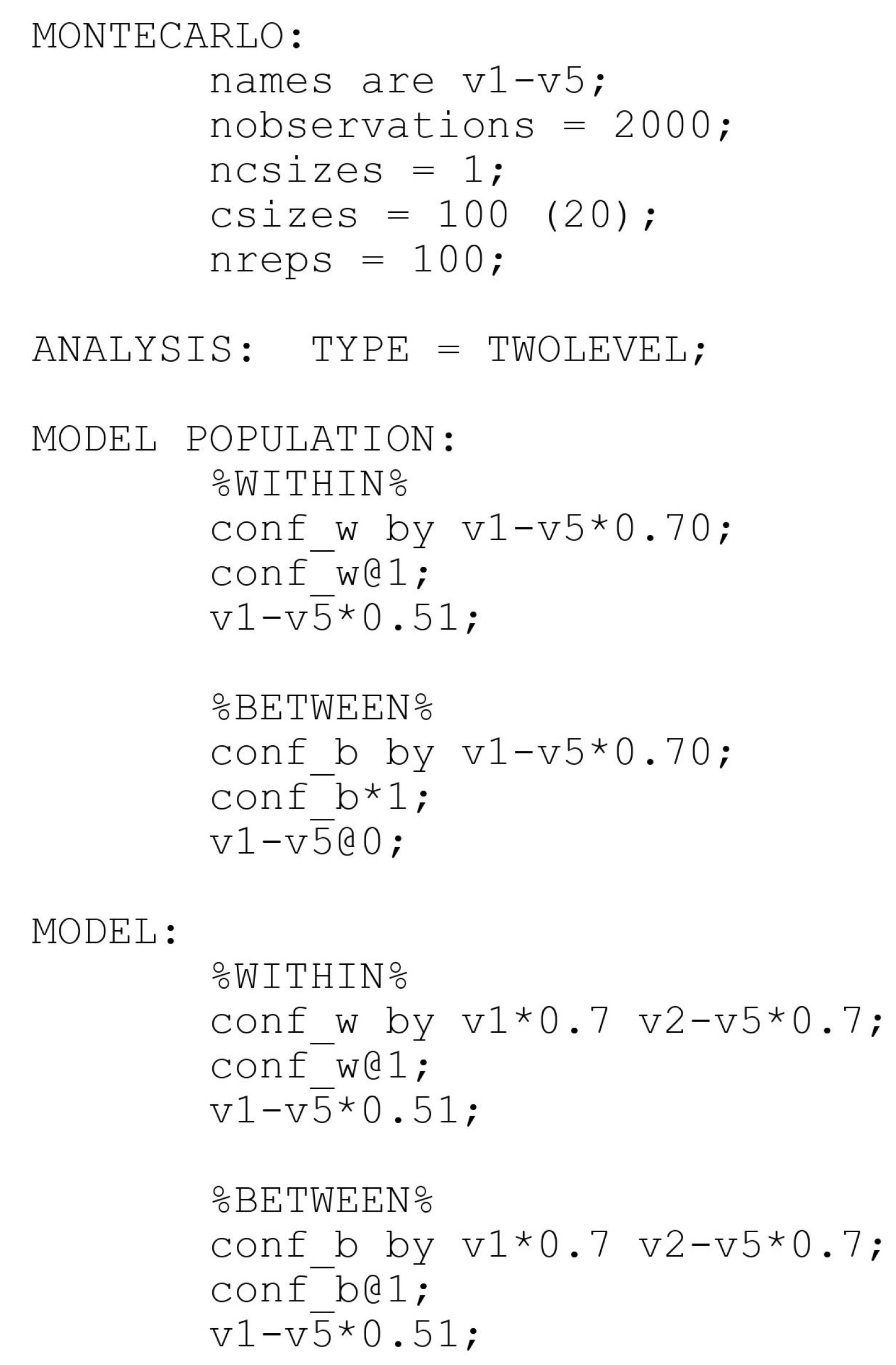
Suppose that a model M yields a solution on the boundary of admissible space of the estimation algorithm. Let q be the number of parameters for which the log-likelihood derivatives are not zero according to the set convergence criterion. In a typical SEM or multilevel model estimation, the number q should be relatively small compared to the total number of model parameters f. Let c be the LRT correction number for model M. As is shown in Jak et al. [1], using c directly is likely to yield an undesirable inflated type-I error for the test of fit where the model M is compared to an unrestricted variance-covariance model. In practical applications, this can lead to confusion. Not only are the maximum-likelihood estimates inadmissible or on the border of admissible space, but the model is rejected as well. The reality might be that certain random effects are simply not needed, while in principle, the model is correct. One general possibility here is to simply fix the problems with model M so that the parameters estimates are admissible. This, however, does not necessarily resolve the problem. It is shown in Jak et al. [1] that simply removing zero residual variances from the model only partially resolves the inflation in the type-I error rates. This is due to the fact that the test of fit uses the correction number not only for model M (which does not have borderline parameters) but also the correction number for the unconstrained variance covariance model (which does have borderline parameters). In general, when model M has an inadmissible solution, the less parsimonious unconstrained model is likely to have an inadmissible solution as well. The unconstrained model will be difficult to resolve via model modification. Typically, in SEM software packages, this unconstrained model is not directly controlled in the model estimation. Therefore, a general LRT correction factor modification is needed that resolves problems not just with the estimated SEM model but also applies to the unconstrained variance covariance model. Below, we describe such a modification for any model M.

Denote by $M^{*}$ the model where the problematic q parameters are held fixed to the model M estimates. Let $c^{*}$ be the correction factor for model $M^{*}$. This correction factor satisfies the asymptotic theory assumptions as no parameter is on the border. One possibility to adjust the LRT correction number is to simply use $c^{*}$ instead of c for model M. Another possibility is to use

$$c=\frac{f-q}{f}{c}^{*}+\frac{q}{f}.$$

(10)

The interpretation of this second approach is that the problematic parameters provide no evidence to correct the LRT test, and thus, they contribute 1 in the numerator of Equation (5) as they do in the denominator. This modified correction factor is a weighted average between the correction factor $c^{*}$ and 1 where the weights correspond to the number of problematic parameters in the model. This second approach is implemented in Mplus 8.7.

In practical applications, it is not unusual that problematic parameters occur. In most situations, however, the number of problematic parameters will be small, and thus, the modified correction number will not change substantially. In an experimental study that encompasses over 10,000 SEM model estimations that the authors have accumulated over the years, some based on real data and some based on simulated data, only about 40 examples needed modifications for their correction number. In most of these, the modification occurred for the unconstrained model, which tends to be more vulnerable to borderline solutions. The most common parameter to be on the border of the admissible space was the zero residual variance on the between level as well as between-level correlation parameters approaching the value of 1. In these 40 examples, the modifications of the LRT correction factor were small, particularly so in real data examples, where only a small portion of the parameters are at the border of the admissible space. Because the corrections tend to be small in real data populations, only rarely will the correction actually impact the ultimate decision on model fit. In the experimental study, none of the real data examples actually reversed the decision on model fit because of the modified correction factor.

The examples that had the most significant modifications were simulated examples that resemble the examples considered in Jak et al. [1]. These examples are characterized by the fact that all random effects on the between level are fully correlated in the data generation model, i.e., all the correlations are 1 in ${\mathsf{\Sigma }}_B$ because ${\theta }_B=0$. In practical examples, this is unlikely to happen. In the two-level example used in Jak et al. [3], when ${\theta }_B=0$, all correlation parameters in ${\mathsf{\Sigma }}_B$ are 1. Since the correlation parameters on the between level are approximately half of the parameters in the unconstrained variance covariance model, which means that approximately 50% of all model parameters are on the border of admissible space. While the simulations in Jak et al. [1] undeniably reveal the need for a modified correction number in such extreme situations, we do not expect that the modified correction number will have a substantial impact on real data applications. For real data applications, when estimating the unconstrained variance covariance matrix, the correlations are often very high, but not more than a few of these correlations will be estimated sufficiently close to 1 to become problematic parameters. Similarly, when estimating a factor analysis model with free residual variances on the between level, the residual variances are often small and insignificant. It is unusual, however, to have more than a few of these residual variances be estimated to 0 or negative values. To be clear, we are not arguing here that the estimated models presented in Jak et al. [3] are uncommon. On the contrary, these models are quite common. We are simply observing that in real data populations, the between-level components are unlikely or rarely as perfectly correlated as they are in the simulated data used in that article. Nevertheless, the simulation studies conducted in Jak et al. [1] are very common and are often used for power analysis related to real data applications (see Muthén and Muthén [9]). Thus, real data analysis may indirectly be affected by the inflation of the type-I error related to power analysis.

The Mplus implementation of the new log-likelihood correction factor does not require additional commands in the Mplus input file. Mplus will automatically check for problematic parameters and will engage the corrective procedure if such parameters are found. No syntax changes are necessary to obtain the new corrected results.

5. Simulation Study

To illustrate the efficacy of the modified correction number, we compare the results obtained in Mplus 8.6 and Mplus 8.7 on the simulation reported in Table 6 from Jak et al. [1]. Note, however, that when the between-level residual variance ${\theta }_B$ is positive in the generating model, the true model parameters do not represent a borderline solution. The true parameter values are in the interior of the parameter space. In that case, the LRT correction factor modification is not used, and the chi-square values will be identical in Mplus 8.6 and Mplus 8.7. In those situations, as reported by Jak et al. [1] and shown in Table 6, the robust chi-square yields an accurate type-I error. For a correct estimated model, the rejection rates are near the nominal value of 5%. For an incorrect estimated model, the rejection rates are 100%. To be more specific, these simulation studies are given in rows 1–6 and rows 13–18 in Table 6.

Here, we focus on rows 7–12 and rows 19–24 where the generating model uses ${\theta }_B=0$. In all of these rows, the estimated models should not be rejected. The models should not be rejected even for rows 19–24 where the generating model has two factors on the between level. That is because the generating loading parameters are identical across indicators for both factors. This implies that the model is equivalent to a one-factor model on the between level, and therefore, all of the estimated models are correct. We expect to see a rejection rate near the nominal value of 5% for all these models. The results of this simulation study are presented in

Table 1. Rejection rates of the robust chi-square test of fit corresponding to Table 6, rows 7–12 and 19–24 in Jak et al. [1], ${\theta }_B=0$ for the generating model.

Generating Model	Estimated Model	Estimated Model ${\mathit{\theta }}_{\mathit{B}}$	Mplus 8.6 EMA	Mplus 8.7 EMA	Mplus 8.6 QN	Mplus 8.7 QN
Config	Uncon	${\theta }_B>0$	0.46	0.03	-	-
Config	Uncon	${\theta }_B=0$	0.17	0.03	0.17	0.03
Config	Config	${\theta }_B>0$	0.36	0.05	-	-
Config	Config	${\theta }_B=0$	0.10	0.03	0.10	0.03
Config	Shared	${\theta }_B>0$	0.45	0.06	-	-
Config	Shared	${\theta }_B=0$	0.17	0.07	0.11	0.05
Shared	Uncon	${\theta }_B>0$	0.46	0.03	-	-
Shared	Uncon	${\theta }_B=0$	0.17	0.03	0.17	0.03
Shared	Config	${\theta }_B>0$	0.35	0.05	-	-
Shared	Config	${\theta }_B=0$	0.09	0.03	0.09	0.03
Shared	Shared	${\theta }_B>0$	0.41	0.08	-	-
Shared	Shared	${\theta }_B=0$	0.19	0.05	0.10	0.03

for the EMA and the QN algorithm. The QN algorithm does not converge in all the cases when the residual variances are estimated as free parameters. The EMA algorithm converges in all situations as it is designed to better deal with solutions that are on the border of the admissible space. The results show that the modified correction number implemented in Mplus 8.7 yields accurate results for the robust chi-square test of fit with both the EMA and the QN algorithms. The Mplus input file used to obtain the results in the first row of Table 1 is included in Appendix A.

6. Conclusions

In this article, we describe some of the challenges that can be encountered when using the robust chi-square method in extreme situations where the model parameter estimates are at the border of the admissible parameter space. We also describe a modification of the robust chi-square test of fit, implemented in Mplus 8.7, which eliminates the inflation in the type-I error described in Jak et al. [1].

References

1. Jak, S.; Jorgensen, T.D.; Rosseel, Y. Evaluating cluster-level factor models with lavaan and Mplus. Psych 2021, 3, 134–152. [Google Scholar] [CrossRef]
2. Muthén, B.O.; Satorra, A. Multilevel aspects of varying parameters in structural models. In Multilevel Analysis of Educational Data; Academic Press: Cambridge, MA, USA, 1989; pp. 87–99. [Google Scholar]
3. Muthén, B.O. Mean and Covariance Structure Analysis of Hierarchical Data; UCLA Statistics Series #62; UCLA: Los Angeles, CA, USA, 1990. [Google Scholar]
4. Muthén, L.K.; Muthén, B.O. Mplus User’s Guide, 8th ed.; Muthén & Muthén: Los Angeles, CA, USA, 2017. [Google Scholar]
5. Dempster, A.P.; Laird, N.M.; Rubin, D.B. Maximum Likelihood from Incomplete Data via the EM Algorithm. J. R. Stat. Soc. Ser. B 1977, 39, 1–38. [Google Scholar]
6. Satorra, A.; Bentler, P.M. Scaling Corrections for Chi-Square Statistics in Covariance Structure Analysis. In Proceedings of the Business and Economic Statistics Section of the American Statistical Association, Atlanta, GA, USA, 24–28 August 1988; pp. 308–313. [Google Scholar]
7. Yuan, K.; Bentler, P.M. Three Likelihood-Based Methods for Mean and Covariance Structure Analysis With Nonnormal Missing Data. Sociol. Methodol. 2000, 30, 167–202. [Google Scholar] [CrossRef]
8. Asparouhov, T.; Muthén, B. Multivariate Statistical Modeling with Survey Data. In Proceedings of the Federal Committee on Statistical Methodology (FCSM) Research Conference, Washington, DC, USA, 14 November 2005. [Google Scholar]
9. Muthén, L.K.; Muthén, B.O. How to use a Monte Carlo study to decide on sample size and determine power. Struct. Equ. Model. 2002, 4, 599–620. [Google Scholar] [CrossRef]