Next Article in Journal / Special Issue
cdcatR: An R Package for Cognitive Diagnostic Computerized Adaptive Testing
Previous Article in Journal
The Sociotype of Dermatological Patients: Assessing the Social Burden of Skin Disease
Previous Article in Special Issue
Using the Effective Sample Size as the Stopping Criterion in Markov Chain Monte Carlo with the Bayes Module in Mplus
 
 
Please note that, as of 22 March 2024, Psych has been renamed to Psychology International and is now published here.
Article

Predicting Differences in Model Parameters with Individual Parameter Contribution Regression Using the R Package ipcr

by
Manuel Arnold
1,2,*,
Andreas M. Brandmaier
2,3 and
Manuel C. Voelkle
1
1
Psychological Research Methods, Department of Psychology, Humboldt-Universität zu Berlin, 12489 Berlin, Germany
2
Max Planck UCL Centre for Computational Psychiatry and Ageing Research, 14195 Berlin, Germany
3
Center for Lifespan Psychology, Max Planck Institute for Human Development, 14195 Berlin, Germany
*
Author to whom correspondence should be addressed.
Psych 2021, 3(3), 360-385; https://doi.org/10.3390/psych3030027
Submission received: 3 June 2021 / Revised: 26 July 2021 / Accepted: 28 July 2021 / Published: 6 August 2021

Abstract

:
Unmodeled differences between individuals or groups can bias parameter estimates and may lead to false-positive or false-negative findings. Such instances of heterogeneity can often be detected and predicted with additional covariates. However, predicting differences with covariates can be challenging or even infeasible, depending on the modeling framework and type of parameter. Here, we demonstrate how the individual parameter contribution (IPC) regression framework, as implemented in the R package ipcr, can be leveraged to predict differences in any parameter across a wide range of parametric models. First and foremost, IPC regression is an exploratory analysis technique to determine if and how the parameters of a fitted model vary as a linear function of covariates. After introducing the theoretical foundation of IPC regression, we use an empirical data set to demonstrate how parameter differences in a structural equation model can be predicted with the ipcr package. Then, we analyze the performance of IPC regression in comparison to alternative methods for modeling parameter heterogeneity in a Monte Carlo simulation.

1. Introduction

A fundamental assumption of parametric modeling is that the model parameters represent all individuals in the sample. However, populations investigated in the behavioral sciences and related fields are rarely homogeneous and instead are often characterized by substantial differences between individuals or groups. For example, heterogeneity may reflect age differences in cognitive functioning (e.g., [1]) and differences in the prevalence of depression between women and men (e.g., [2]). Overlooking such heterogeneity results in an incomplete model with potentially biased parameter estimates and may lead to false-positive or false-negative findings [3,4]. Conversely, discovering and explaining heterogeneity can substantially support theory building.
Individual and group differences can often be accounted for with additional covariates such as contextual or background variables. In practice, researchers routinely probe the effects of potentially important covariates by using them as moderator variables or by estimating group-specific parameter values using pre-defined grouping variables. However, researchers are often limited to investigate only certain types of model parameters, depending on the choice of modeling technique. For instance, in regression models such as linear regression, generalized linear regression, and linear mixed models, differences in regression coefficients can be studied by simply adding covariates with main and interaction effects. On the contrary, uncovering heterogeneity in the variance parameter of the regression errors (or in the different variance parameters of a mixed model) with covariates is much more challenging. For example, in the statistical programming language R [5], neither the built-in function lm (for fitting linear regression models) or the functions of the widely used lme4 package (for fitting mixed models; [6]) allow for ways to explain individual and group differences in the variance parameters in the model with covariates. Other modeling frameworks, such as structural equation modeling (SEM; [7,8]), offer the user more flexibility to incorporate covariates and investigate their effects on all model parameters. One popular method for investigating the effect of a discrete covariate is the use of multigroup structural equation models (MGSEMs, [9]). MGSEMs allow estimating SEMs with different parameter values across the levels of a grouping variable. If the covariate under investigation is continuous, one possible way to assess its effect is to include it into the SEM as a moderator variable by specifying a SEM with an interaction term (e.g., [10]). MGSEMs and SEMs with interactions are best suited in situations with a priori knowledge about the sources of heterogeneity and a clear set of target parameters. However, both approaches can quickly become impractical in an exploratory analysis of the potential effects of a larger number of covariates on multiple model parameters. As MGSEMs and SEMs with interactions are usually conducted by looking at the effects of one covariate at a time, many SEMs need to be specified, estimated, and evaluated. Moreover, exploring potential interactions between covariates may result in MGSEMs with too sparse groups or overly complex interaction models with too many parameters to be stably estimated.
As an alternative procedure to exploring the effects of covariates by adding them to the model, we introduced individual parameter contribution (IPC) regression [11,12]. IPC regression allows determining whether and how the parameters of a model vary as functions of covariates. IPC regression proceeds in three steps. First, the model is fitted to data. This model represents a given scientific theory, encompassing all variables that pertain to this theory and for which hypothesized relationships can be specified. Second, individual contributions to the model parameters are calculated. These IPCs are rough approximations of individual-specific parameter values. Third and last, the IPCs are regressed on a set of covariates such as discrete grouping variables or continuous variables to investigate whether any of these covariates predict differences in the parameters. The result of an IPC regression analysis may be used to explore predictors of parameter heterogeneity, generate new hypotheses about predictors of individual or group differences in model parameters, and may ideally help revise the substantive theory. To perform IPC regression in practice, we provide the R package ipcr.
IPC regression is a general, flexible, simple, and computationally efficient method. In principle, IPC regression allows investigating all types of model parameters of a parametric model. For instance, IPC regression makes it feasible to predict differences in certain types of model parameters, such as the residual variance parameters in regression models, which would not be possible by adding covariates directly to the model. Furthermore, IPC regression encompasses both discrete grouping variables as well as continuous covariates. This flexibility regarding the measurement level of the covariates appears particularly advantageous when working with SEMs. For SEMs, the effects of discrete and continuous covariates are often studied with different techniques, that is, either with MGSEMs (for discrete variables) or SEMs with interactions (for continuous variables). With IPC regression, we can leverage the same approach for studying covariates with different levels of measurement. Although the derivation of the IPCs is a little more involved, a basic understanding of linear regression is sufficient to perform IPC regression in practice. A final key feature of IPC regression is a clear separation between model estimation and the investigation of parameter differences. This separation is especially advantageous when the model is complex and hard to estimate (either in the sense of computation time or convergence problems) because assessing parameter heterogeneity does not involve repeated re-specification and re-estimation.
IPCs are calculated by transforming the partial derivative of an objective function with respect to the parameters. Objective functions such as the well-known log-likelihood function are used to estimate model parameters. Various statistical procedures analyze the derivative of an objective function to assess the fit of a statistical model. In the SEM framework, the modification index (MI; [13]) uses the derivative to approximate how much the fit of a model would change after a new parameter is added to the model. As an extension to the MI, which is merely a test statistic, the expected parameter change (EPC; [14,15]) has been put forward for obtaining a direct estimate of the added parameter. Although the MI and EPC aim to quantify specification errors, Oberski [11] demonstrated that the MI and EPC for MGSEMs correspond to IPC regression under certain conditions. However, this equivalency ends in situations that cannot be handled by MGSEMs, such as continuous or multiple covariates, making IPC regression a much more flexible method for the investigation of heterogeneity. Other methods that analyze partial derivatives are structural change tests (e.g., [16,17]). Originally used in the detection of change points in time series analysis [18], structural change tests have been recently popularized by Merkle and Zeileis [19] and Merkle et al. [20] to uncover parameter heterogeneity in psychometric models. The difference between structural change tests and IPC regression is that structural change tests provide formal tests whether the parameters of a model are invariant with respect to a covariate. In contrast, IPC regression seeks to model the relationships between parameters and covariates by means of linear regression.
The purpose of this study is threefold. First, we introduce the ipcr package, which offers functions to perform IPC regression in R. Second, we expand upon earlier research, which focused on predicting differences in SEM parameters, by discussing how IPC regression can be used to investigate a much broader range of parametric models. Third, we compare the performance of IPC regression to established methods in four small Monte Carlo simulations. The remainder is structured as follows: Section 2 illustrates IPC regression by means of an instructive example. Section 3 deals with the theory behind IPC regression. This section is optional and addresses readers that are interested in more technical details. Section 4 gives an overview of the ipcr package. Section 5 illustrates how the ipcr package is applied in practice based on data from the lavaan package [21]. Section 6 presents the simulation results. Finally, this study concludes in Section 7 with a discussion of the method and the simulation results.

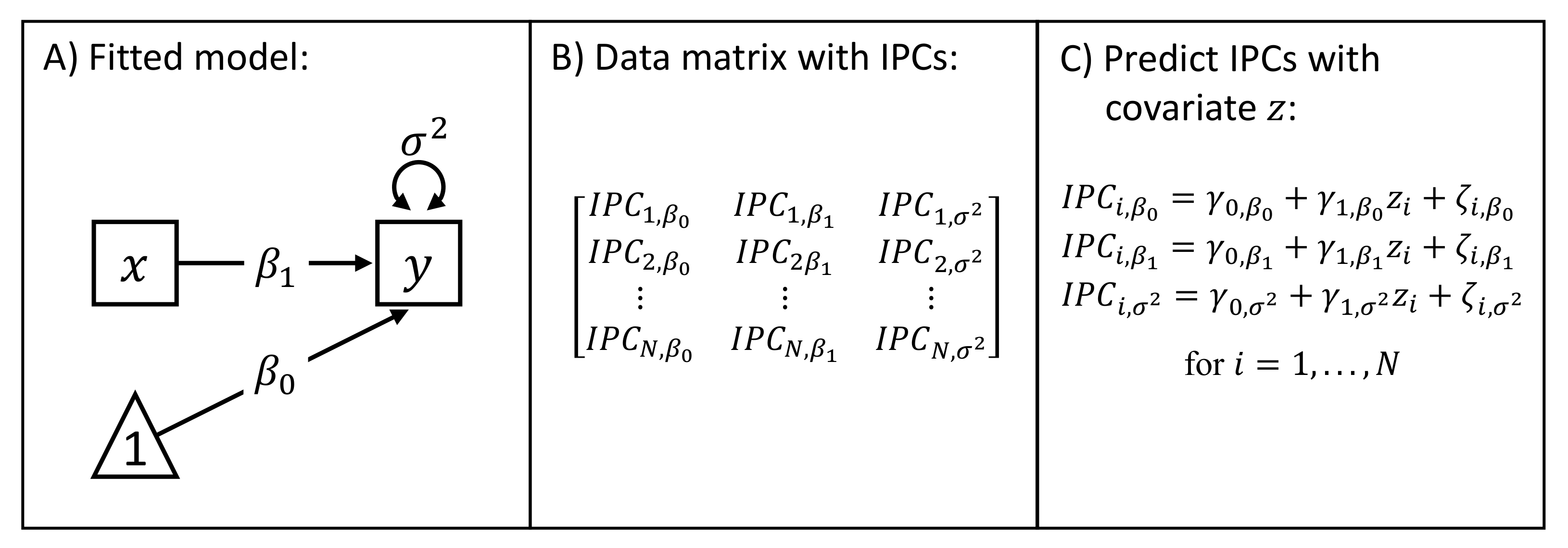
2. Introductory Example

In the following, we illustrate the rationale behind IPC regression with a simple regression example. Let us assume we want to predict an outcome variable y as a linear function of a single explanatory variable x. The corresponding simple linear regression model can be defined as
y i = β 0 + β 1 x i + ε i , i = 1 , , N .
This regression model contains the parameters β 0 , β 1 , and σ 2 . The regression coefficients β 0 and β 1 denote the intercept and slope of the regression line. σ 2 is the variance of the regression errors ε ; that is, the part of the variability in the outcome y that is not explained by the explanatory variable x. Unbiased and efficient parameter estimates can be obtained by employing the ordinary least squares (OLS) estimation method.
Further, we suspect that our model parameters could vary with respect to a covariate z. One way to assess the influence of z would be to simply add the covariate to our model by specifying a direct effect from z on y and an interaction effect between z and x. The direct and interaction effects would then tell us how β 0 and β 1 are influenced by z. However, adding the covariate to the model does not enable us to quantify its influence on the variance parameter σ 2 . On the other hand, IPC regression offers a way to estimate the effect of z on σ 2 .
An IPC regression analysis involves three steps. In the first step, the simple linear regression model defined in Equation (1) is fitted to data. Generally, models investigated with IPC regression consist solely of variables important to one’s scientific theory. Therefore, covariates are usually not included in the first-step model but are used later as predictor variables in step three. In the second step, a new data matrix of IPCs is calculated. Every row of this data matrix corresponds to one individual and every column to one parameter. For example, row i contains the values of the three model parameters specific to individual i. The IPCs of a single individual are usually too noisy to be useful estimates of individual-specific parameters. However, regressing the IPCs on covariates averages out this noise and may reveal meaningful differences in the parameters. Figure 1 illustrates the three steps of IPC regression.
The IPC regression coefficients are interpreted as in any linear regression model. The IPC regression slope γ 1 , β 0 represents the change in the intercept β 0 of the first-step model for a one-unit change in the covariate z. Further, the IPC regression slope γ 1 , β 1 indicates how z moderates the effect of the explanatory variable x on the outcome y. Finally, γ 1 , σ 2 represents the relationship between z and the variance of the regression errors σ 2 . A positive relationship indicates that individuals with smaller covariate values exhibit a smaller error variance and are therefore closer to the regression line, whereas individuals with larger values show more unexplained variability.
As in standard regression analysis, a t-test can be carried out to test the null hypotheses γ 0 = 0 and γ 1 = 0 . Testing γ 1 = 0 can be seen as a test of parameter homogeneity with respect to the covariate z, and rejecting it implies that the parameter under investigation is not constant across individuals. It should be noted that the errors ζ i of the IPC regression equations are usually not normally distributed, even if the original data used for model fitting are normal. Therefore, the standard errors of the IPC regression estimates may be inaccurate in small samples.
Figure 1 shows a simplistic example with a single covariate. In practice, one might be interested in investigating the effects of multiple covariates and their interactions or estimating non-linear relationships between the model parameters and covariates by adding quadratic and cubic terms. All these techniques work exactly as in standard linear regression.

3. Derivation and Properties of Individual Parameter Contributions

In the following, we will first derive the IPCs in very general terms and then give more specific results for linear regression models. Further derivations for SEMs are provided by Arnold et al. [12]. Readers uninterested in technical details may skip this section.

3.1. Calculation of the Individual Parameter Contributions

In brief, IPCs are calculated by transforming the partial derivative of a case-wise objective function with respect to the parameters. More formally, let f ( θ ) be an objective function used to estimate a q-variate vector of model parameters θ based on data from N individuals. Typical examples for such an objective function are the sum of squared residuals (SSE) for linear regression models or the normal-theory maximum-likelihood fitting function for SEMs. The model parameter estimates θ ^ are obtained by minimizing the objective function, that is,
θ ^ = argmin θ f ( θ ) .
In practice, f is minimized by finding the roots (the zeros) of the partial derivative of the objective function. Thus, parameter estimates θ ^ can be found by solving the first-order condition
S ( θ ^ ) = 0 ,
where
S ( θ ) = f ( θ ) θ ( 1 ) f ( θ ) θ ( q )
is the partial derivative of the objective function f ( θ ) with respect to the parameters θ . Additional steps may be required to ensure that the parameter estimates are associated with the global minimum, depending on the type of objective function. In maximum likelihood estimation, the partial derivative defined in Equation (4) is known as the score. We will use this term to refer to the derivatives of all kinds of objective functions in the following.
The idea behind the derivation of the IPCs is simple. Instead of employing a score S ( θ ) , which takes information from all individuals into account to estimate a single set of parameters, we specify individual-specific scores to find individual-specific parameter estimates. In greater detail, let S i ( θ ) denote the score that uses only data from individual i. Hypothetically, solving S i ( θ ^ i ) = 0 would yield a vector of parameter estimates θ ^ i specific to individual i. Unfortunately, the system of equations S i ( θ ^ ) = 0 is undetermined for most objective functions because there are more unknown parameters than individual-specific data. However, we can approximate the individual scores by combining individual data with information from the model.
Individual scores can be approximated through linearization. The equation for the linearization of the score S ( θ ) at the model parameter estimates θ ^ is:
S ( θ ) S ( θ ^ ) + H ( θ ^ ) θ θ ^
The first term, which is the intercept of the linear approximation, is just the score itself, evaluated at the parameter estimates. From Equation (3), we can see that this intercept is always zero. The function
H ( θ ) = 2 f ( θ ) θ θ
is the Hessian matrix of second-order partial derivatives of the objective function with respect to the parameters. In the equation above, H ( θ ) is the slope of the linearized score.
In the next step, we individualize this linear approximation of the score by replacing the sample score S ( θ ^ ) with an individual-specific score S i ( θ ^ ) . As a result, the intercepts of the individual score approximations are no longer zero but fluctuate around zero. In contrast to the sample score S ( θ ^ ) , the sample Hessian matrix H ( θ ^ ) cannot be individualized as that would destabilize the approximation. Therefore, we are borrowing the Hessian matrix from the complete sample. As a result, the individualized approximated scores
S i ( θ ^ ) + 1 N H ( θ ^ ) θ θ ^ , for i = 1 , , N ,
all have the same slope.
Finally, finding the roots of these individualized scores yields the IPCs.
0 = S i ( θ ^ ) + 1 N H ( θ ^ ) I P C i ( θ ) θ ^ I P C i ( θ ^ ) = θ ^ 1 N H ( θ ^ ) 1 S i ( θ ^ )
The mean and variance of the IPCs correspond to well-known quantities. It follows directly from Equation (3) that the mean of the IPCs equals the parameter estimates; that is, M M 1 / N i = 1 N I P C i ( θ ^ ) = θ ^ . Calculating the variance of the IPCs yields the following sample estimate of the so-called sandwich estimator of the covariance matrix of the parameters (see [22]):
Var ^ I P C i ( θ ^ ) = 1 N H ( θ ^ ) 1 1 N i = 1 N S i ( θ ^ ) S i ( θ ^ ) 1 N H ( θ ^ ) 1 = Var ^ ( θ ^ )
Next, we will give more explicit examples by deriving the IPCs to the regression coefficients of the standard multiple linear regression model, using the SSE objective function. The following model
y i = x i β + ε i , i = 1 , , N ,
extends the simple linear regression model in Equation (1) by having p regressors x with a corresponding p-variate vector of regression coefficients β .
To calculate the IPCs to the estimated regression coefficients β ^ , we need the first-order and second-order partial derivatives of the objective function. The SSE objective function minimizes the sum of the squared differences between the observed values of the outcome variable y and the predicted values based on the regression model. Formally, the SSE objective function is defined as
f ( β ) = i = 1 N y i x i β 2 .
The first-order and second-order derivatives of the objective function are:
S ( β ) = 2 i = 1 N x i y i + x i x i β
H ( β ) = 2 i = 1 N x i x i
Thus, the IPCs of individual i to the estimated regression coefficients β ^ are given by
I P C i ( β ^ ) = β ^ 1 N H ( θ ^ ) 1 S i ( β ^ ) = β ^ 2 N i = 1 N x i x i 1 2 x i y i + 2 x i x i β ^ = β ^ + 1 N i = 1 N x i x i 1 x i y i 1 N i = 1 N x i x i 1 x i x i β ^ = 1 N i = 1 N x i x i 1 x i y i + I p 1 N i = 1 N x i x i 1 x i x i β ^ ,
where I p denotes an identity matrix of order p.
Equation (14) allows us to illustrate the behavior of IPCs from groups of the sample. Let G be the index set of a group of n G individuals with the same values in their covariates. Consider the following group-specific mean:
1 n G j G I P C j ( β ^ ) = 1 N i = 1 N x i x i 1 1 n G j G x j y j + I p 1 N i = 1 N x i x i 1 1 n G j G x j x j β ^
In the above equation, the outer product of the regressors x x plays an important role. If the group-specific average of the outer product is identical to the outer product averaged over the complete sample, then the first term of Equation (15) equals the OLS estimate of the group-specific regression coefficients and the second term is zero. Therefore, the mean of the IPCs from this group will be an unbiased estimator of the group-specific regression coefficients. However, if the group-specific average of the outer product differs from the outer product averaged over the complete sample, then the first term will not be identical to the OLS estimate and the second term will not drop out. Thus, group differences in the outer product bias the IPCs. The size of this bias is proportional to the size of the differences in the outer products. These insights also apply to other model classes. Generally speaking, the bias of the IPCs increases with the amount of heterogeneity in the data [12]. In homogeneous samples, the IPCs are guaranteed to be unbiased.

3.2. Bias Correction Procedure

Arnold et al. [12] suggested a correction procedure termed iterated IPC regression that removes bias in the IPCs in a stepwise fashion. Iterated IPC regression proceeds as follows: first, the model is fitted, and standard IPC regression is performed. Second, individual-specific model parameters are predicted using the coefficients of the IPC regression equations. Third, these individual-specific model parameters are used to re-estimate the IPCs. The third step reduces some bias in the IPCs as the re-estimated IPCs are closer to the true individual-specific parameter values. By iterating over steps 2 and 3, the bias of the IPCs usually vanishes completely and the IPC regression estimates converge to unbiased estimates of the individual parameters. In a simulation study, Arnold et al. [12] compared both IPC regression approaches by predicting group differences in dynamic panel models. In contrast to standard IPC regression, whose estimates were slightly biased, the iterated algorithm provided nearly unbiased but slightly less precise estimates. Iterated IPC regression is implemented in the ipcr package. However, the iterated algorithm is limited to SEMs at present.

4. The ipcr Package: Overview and Installation

The ipcr package supplies functions for calculating IPCs and performing IPC regression. To a large extent, ipcr relies on infrastructure provided by the sandwich package [23]. sandwich allows users to estimate a wide variety of model-robust covariance estimators. The sandwich package contains the generic functions estfun() and bread() used as the building blocks to calculate the IPCs. estfun() returns the case-wise partial derivatives of the objective function with respect to the model parameters (see Equation (4) for the sum of the case-wise scores). bread() extracts an estimator for the expectation of the negative derivative of the objective function; usually the Hessian as defined in Equation (6).
Since the ipcr package was first introduced by Arnold et al. [12] to investigate parameter differences in SEMs fitted with the OpenMx package [24], support for various parametric models has been added. Now, ipcr can also be used to investigate SEMs fitted with the lavaan package [21]. Other than SEMs, linear and generalized regression models fitted by R’s built-in lm() and glm() functions are supported. Moreover, by using some extractor functions provided by the merDeriv package [25], ipcr can also be applied to study parameter heterogeneity in Gaussian linear mixed models fitted with the lme4 package [6]. Other notable new features are better plotting capabilities and regularized IPC regression.
ipcr can be downloaded from GitHub https://github.com/manuelarnold/ipcr (accessed on 5 August 2021). The easiest way to obtain ipcr is via the devtools package [26]. To install and load ipcr within R, simply use the following commands:
R> library("devtools")
R> install_github("manuelarnold/ipcr")
R> library("ipcr")

5. Application

This section demonstrates how parameter differences can be detected and predicted with the ipcr package, using the HolzingerSwineford1939 data set included in the lavaan package.

5.1. Data Overview

HolzingerSwineford1939 is a classic data set that has often been used to illustrate different SEM applications. It consists of mental ability test scores of 301 seventh-grade and eighth-grade children from two different schools and additional variables indicating the children’s sex, age, school, and grade. For the sake of simplicity, we limit this demonstration to a subset of the variables. We will use three visual ability test scores to fit a confirmatory factor analysis (CFA) model. Then, we use sex, age, school, and grade as IPC regression predictor variables to predict differences in the model. The variables are briefly described in Table 1.

5.2. Data Pre-Processing

Below, we explain how missing data can be handled and show some preparation steps that facilitate the interpretation of IPC regression. First, we load the lavaan package that contains the data set. Then, we store the data set under a new variable name:
R> library("lavaan")
R> HS_data <- HolzingerSwineford1939
The students’ age is stored in two different variables: ageyr measures the age in completed years, and the variable agemo contains the additional months. Next, we combine this information into a single variable that measures the students’ age in months:
R> HS_data$age_months <- 12 * HS_data$ageyr + HS_data$agemo
Currently, the ipcr package requires the data used to fit the model and covariates to be complete, that is, without any missing values. In the cases of the HolzingerSwineford1939 data set, there is just a single missing value in the covariate grade. In order to keep this illustration simple, we will exclude the individual with the missing value from the data set by deleting the corresponding row in the data.frame. However, it has long been known that list-wise deletion is not optimal, and users with incomplete data sets might consider more sophisticated methods such as multiple imputation (see [27,28]) to deal with missing values. Here, we delete the incomplete row with the following command:
R> HS_data <- HS_data[complete.cases(HS_data), ]
As in standard linear regression, the interpretation of the intercept can often be facilitated by centering the predictor variables at their means. After centering the covariates, a regression intercept represents the estimated parameter value for individuals with an average value on all covariates. The effects of categorical covariates, such as grouping variables, can be studied by encoding them as dummy variables. In the following, we center the covariate months and change the coding of all categorical covariates to either 0 or 1. We store the resulting covariates in a new data.frame called covariates:
R> covariates <- data.frame(sex = HS_data$sex - 1,
+                           months = scale(HS_data$age_months,
+                                          center = TRUE,
+                                          scale = FALSE),
+                           school = as.numeric(HS_data$school) - 1,
+                           grade = HS_data$grade - 7)

5.3. Fitting the Model

After the data have been prepared, we fit a CFA model using the cfa function from lavaan. The CFA consists of a latent variable, indicating the students’ visual ability, measured by three manifest variables x1, x2, and x3. Figure 2 shows a graphical representation of the model. The corresponding lavaan syntax for specifying this model is as follows:
R> model_visual <- ’visual =~ x1 + x2 + x3’
Figure 2. Path diagram of the CFA model. The parameters λ 1 and λ 2 denote factor loadings, ϕ represents the variance of the latent variable V, and ψ 1 , ψ 2 , and ψ 3 are measurement error variances.
Psych 03 00027 g002
We can now fit the model:
R> fit_visual <- cfa(model = model_visual, data = HS_data)
The model contains 6 free parameters: 2 factor loadings (the factor loading of x1 is fixed at 1 and the loadings of x2 and x3 are estimated), 1 latent variance parameter, and 3 residual variance parameters of the manifest variables. Since the model has zero degrees of freedom and is just identified, we cannot assess its fit.

5.4. Individual Parameter Contribution Regression

The core of the ipcr package is the ipcr() function. ipcr() calculates IPCs for the parameters of a fitted model and, when provided with a data.frame of covariates, performs IPC regression. Other than the ipcr() function, the ipcr package offers the convenience functions get_ipcs() and get_scores(), which return a data.frame of IPCs or scores, respectively.
In the following, we call the ipcr() function to investigate whether and how the parameters of the CFA model for visual abilities vary with respect to the covariates:
R> library(ipcr)
R> ipcr_visual <- ipcr(fit = fit_visual, covariates = covariates)
ipcr() automatically regresses the IPCs of all model parameter estimates on all covariates in the provided data.frame and returns an object of class icpr. The usual R accessor functions such as coef(), fitted(), plot(), predict(), print(), and summary() can be used to extract various information from the ipcr object. To get a first overview, we can plot a heatmap using plot(ipcr_visual) that shows the correlations between the IPCs and covariates (see Figure 3). By specifying the argument print_corr = TRUE, the correlation coefficients are printed on the heatmap. Note that the heatmap depicts the zero-order correlations between IPCs and covariates, whereas IPC regression estimates the partial effects of the covariates on the IPCs. Zero-order correlations and partial effects might differ, especially if some of the covariates are correlated.
More detailed information can be obtained with the summary() function. summary() prints the IPC regression results for each estimated model parameter:
R> summary(ipcr_visual)
Standard IPC regression coefficients:
        Parameter   Covariate Estimate Std..Error t.value Pr...t..
1      visual=~x2 (Intercept)    0.565      0.326   1.732    0.084
2      visual=~x2         sex   -0.253      0.313  -0.809    0.419
3      visual=~x2      months   -0.027      0.016  -1.712    0.088
4      visual=~x2      school    0.037      0.321   0.114    0.909
5      visual=~x2       grade    0.676      0.365   1.853    0.065
6      visual=~x3 (Intercept)    1.301      0.484   2.690    0.008
7      visual=~x3         sex   -1.192      0.464  -2.566    0.011
8      visual=~x3      months   -0.021      0.023  -0.897    0.371
9      visual=~x3      school    0.152      0.477   0.320    0.749
10     visual=~x3       grade    0.722      0.541   1.333    0.184
11         x1~~x1 (Intercept)    1.046      0.288   3.634    0.000
12         x1~~x1         sex   -0.253      0.276  -0.917    0.360
13         x1~~x1      months    0.015      0.014   1.065    0.288
14         x1~~x1      school   -0.069      0.284  -0.242    0.809
15         x1~~x1       grade   -0.093      0.322  -0.287    0.774
16         x2~~x2 (Intercept)    1.305      0.229   5.695    0.000
17         x2~~x2         sex   -0.603      0.220  -2.739    0.007
18         x2~~x2      months    0.003      0.011   0.251    0.802
19         x2~~x2      school    0.325      0.226   1.438    0.151
20         x2~~x2       grade   -0.195      0.257  -0.759    0.448
21         x3~~x3 (Intercept)    0.255      0.269   0.947    0.344
22         x3~~x3         sex    0.341      0.259   1.317    0.189
23         x3~~x3      months   -0.014      0.013  -1.084    0.279
24         x3~~x3      school    0.240      0.266   0.905    0.366
25         x3~~x3       grade    0.149      0.302   0.493    0.622
26 visual~~visual (Intercept)    0.577      0.310   1.864    0.063
27 visual~~visual         sex    0.611      0.297   2.055    0.041
28 visual~~visual      months    0.028      0.015   1.914    0.057
29 visual~~visual      school   -0.108      0.305  -0.353    0.725
30 visual~~visual       grade   -0.650      0.347  -1.875    0.062
The output is structured as follows: The first column contains the names of the model parameters. The second column shows the names of the covariates, where (Intercept) simply refers to the intercept of the corresponding IPC regression equation. The remaining columns display the estimates, standard errors, t-values, and p-values of the IPC regression parameters as in a standard regression output. Using a significance level of α = 0.05 , we infer that there are three significant sex differences: The factor loading of the indicator x3, the error variance of the indicator x2, and the variance of the latent factor differs significantly between girls and boys. The other covariates do not significantly affect the remaining model parameters. The partial effects of the IPC regression equations can be visualized with the plot_differences() function. Figure 4 shows the estimated factor loading of the indicator x3 for different values of the covariates months and sex when all other covariates are zero.
By default, the accessor functions extract information about all model parameters. The output can be limited to a single or a subset of parameters of interest by specifying the parameter argument. For instance, the function call coef(ipcr_visual, parameter = "visual~~visual") shows only the IPC regression estimates for the variance parameter of the latent factor.

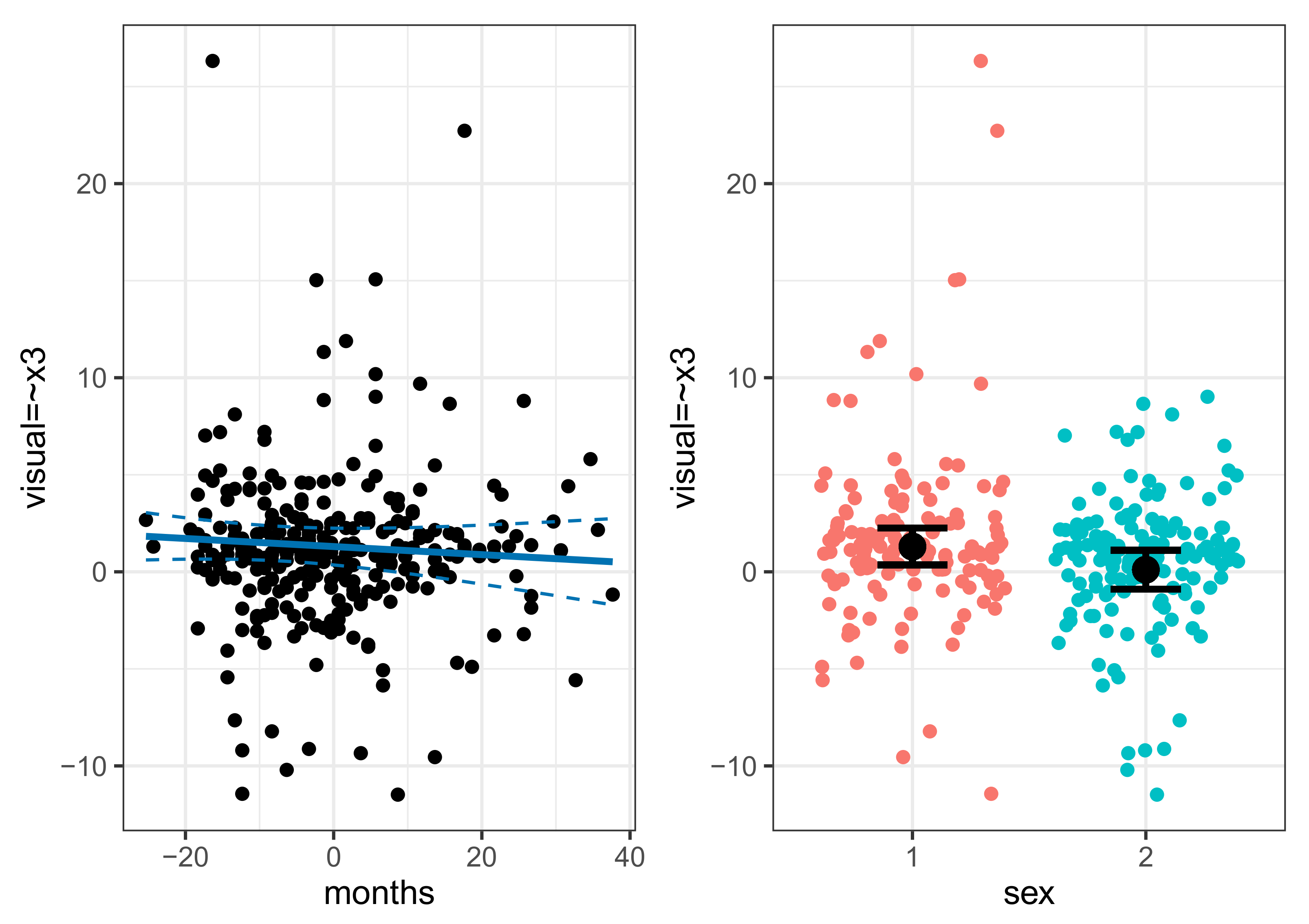
5.5. Non-Linear Effects and Interactions

Since IPC regression is linear regression at its heart, studying non-linear effects or interactions between covariates follows the known logic of adding extra terms to the regression model that are functions of the original covariates. For example, curvilinear relationships between model parameters and covariates can be modeled by adding polynomial terms to the data.frame provided to the covariate argument. Similarly, we can probe interactions between covariates by including product terms. To avoid multicollinearity, we recommend centering all non-dummy covariates used to generate new polynomial or product terms. It is important to remember that more complex models may seem to explain a larger part of the observed variation than simple models unless model selection is performed using approaches that adjust for model complexity or use independent data. A detailed account of modeling non-linear and interaction effects in linear regression models is given by Cohen et al. [29].
Besides exploring relationships between model parameters and covariates, IPC regression also provides means to discover non-linear relationships in the model. For example, consider the simple linear regression model in Equation (1). This model postulates a linear effect of the explanatory variable x on the outcome y denoted by the regression coefficient β 1 . By regressing the IPCs to β 1 on the squared variable x, we can estimate and test the explanatory variable’s potential quadratic effect on the outcome y.

5.6. Bias Correction

IPC regression may provide biased estimates of parameter differences in heterogeneous samples (see [12]). The ipcr package provides a correction procedure called iterated IPC regression that removes the bias in the IPC regression estimates at the cost of adding additional variance. One can perform iterative instead of standard IPC regression by calling the ipcr() function with the additional argument iterate set to TRUE. By default, iterate is set to FALSE, and standard IPC regression is performed. The iterated IPC regression algorithm tries to remove bias in the IPCs in a stepwise fashion and updates the IPC regression estimates as long as the change in any parameter between iterations is smaller than a numerical threshold (by default, the absolute difference needs to become smaller than 1 × 10 4 ). This stopping criterion can be changed via the conv argument of the ipcr() function. Moreover, the user can also specify the maximum number of iterations by changing the max_it argument. By default, the algorithm terminates after 50 iterations. We will later compare the performance of both standard and iterated IPC regression in a series of simulation studies.

5.7. Regularization

If the number of covariates becomes large, there is a risk that we overfit the regression models. A solution to this problem is to make the IPC regression output sparser by coupling IPC regression with the least absolute shrinkage and selection operator (LASSO) [30,31]. LASSO is a widely applied form of regularization that adds a penalty term to the SSE objective function. This penalty term shrinks regression parameters towards zero, thus setting some of them to zero, and, as a result, produces sparser models and reduces overfitting. Note that this approach sets out to minimize prediction error at the cost of regression coefficients becoming biased estimates (see also [32])).
The ipcr package performs LASSO regularized IPC regression by interfacing the glmnet package [33]. More specifically, by setting the argument regularization to TRUE, ipcr() calls the cv.glmnet() function to estimates regularized linear regression models, using k-fold cross-validation. The settings of cv.glmnet() can be changed by providing ipcr() with the specific arguments. By default, 10-fold cross-validation with 100 different values for the penalty term is carried out.
To perform LASSO regularized IPC regression, all covariates need to be standardized beforehand. Standardization prevents LASSO from preferring variables with more variability over variables with less variability. Without standardization, covariates with smaller variances will be penalized more severely than covariates with larger variances. The following command standardizes all covariates:
R> covariates_std <- scale(covariates, center = FALSE, scale = TRUE)
Then, we perform regularized IPC regression and inspect the results with summary():
R> ipcr_visual_reg <- ipcr(fit = fit_visual, covariates = covariates_std,
+                          regularization = TRUE)
R> summary(ipcr_visual_reg)
Regularized standard IPC regression coefficients:
        Parameter   Covariate Estimate
1      visual=~x2 (Intercept)      0.6
2      visual=~x2         sex   -0.142
3      visual=~x2      months   -0.274
4      visual=~x2      school        .
5      visual=~x2       grade    0.403
6      visual=~x3 (Intercept)    1.449
7      visual=~x3         sex   -0.543
8      visual=~x3      months        .
9      visual=~x3      school        .
10     visual=~x3       grade    0.071
11         x1~~x1 (Intercept)    0.835
12         x1~~x1         sex        .
13         x1~~x1      months        .
14         x1~~x1      school        .
15         x1~~x1       grade        .
16         x2~~x2 (Intercept)    1.211
17         x2~~x2         sex   -0.329
18         x2~~x2      months        .
19         x2~~x2      school    0.131
20         x2~~x2       grade        .
21         x3~~x3 (Intercept)    0.627
22         x3~~x3         sex        .
23         x3~~x3      months        .
24         x3~~x3      school        .
25         x3~~x3       grade        .
26 visual~~visual (Intercept)    0.527
27 visual~~visual         sex        .
28 visual~~visual      months        .
29 visual~~visual      school        .
30 visual~~visual       grade        .
The summary() function shows by default the regularized parameter estimates for the penalty term associated with the minimum mean cross-validated error. Parameter estimates for specific penalty terms can be obtained by specifying the s argument in the ipcr() function call and can then be displayed via summary(). In the above output, coefficients that were set to zero are marked with a dot, resulting in a sparse coefficients matrix with the most important coefficients. Standard errors, t-values, and p-values are not shown in the output as they are not provided by glmnet.

6. Simulation Studies

The following series of simulation studies showcases different applications of IPC regression and illustrates the method’s statistical properties. In Simulation I, we revisit the introductory example and predict group differences in the variance of the regression errors of a simple linear regression model. In the subsequent three simulation studies, we turn to SEMs. In Simulation II, we investigate the effect of multiple covariates on the type I error rate. Then, we compare the performance of IPC regression with MGSEMs (Simulation III) and SEMs with interactions (Simulation IV) as established benchmark methods.
All simulations were carried out with R (version 4.0.3). We used R’s built-in lm function to estimate the simple linear regression model in Simulation I. All SEMs were fitted with the lavaan package (version 0.6–7). We used a developmental snapshot of the ipcr package to perform IPC regression (commit: https://github.com/manuelarnold/ipcr/commit/d4132c73b0e05ced1da6be71119d846424a1a3d6 (accessed on 6 August 2021). d4132c7). Throughout all simulations, we set the significance level for all hypothesis tests to 5%. We replicated all experimental conditions 1000 times. The simulation scripts and complete simulation results can be found in our online Supplementary Materials (https://osf.io/p5xrk accessed on 6 August 2021).

6.1. Simulation I: Simple Linear Regression Model
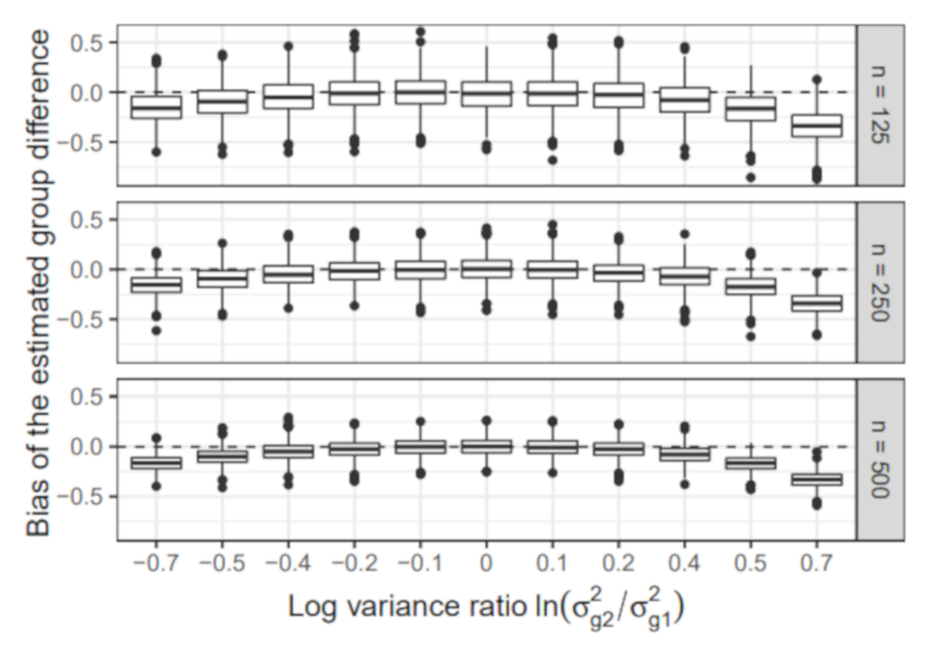
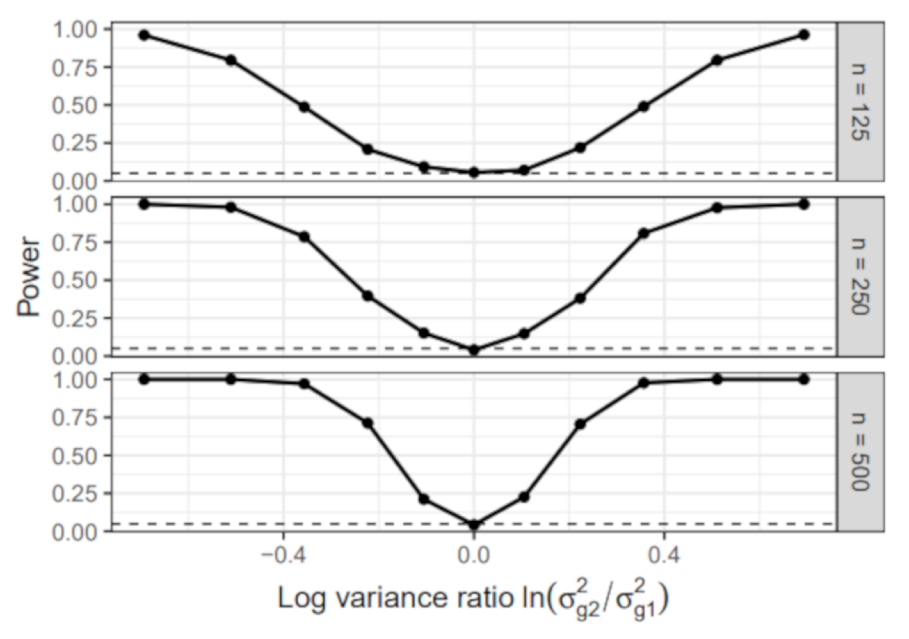
Simulation I assessed how well IPC regression could predict group differences in a simple linear regression model such as the one shown in Equation (1). We sampled the data from a two-group population with a group difference in the error variance σ 2 . This simulation setup corresponds to a situation in which the reliability of the outcome variable differs between groups. For example, such group differences are often encountered in cross-cultural samples (e.g., [34]). If overlooked, the group differences would bias standard errors and render the OLS estimator inefficient. The remaining model parameters, the intercept β 0 and the slope β 1 , did not vary between groups and were set to 1 and 0.5, respectively. In every simulation replication, we simulated data, fitted the linear regression model while ignoring the group difference, and then recovered the group difference with IPC regression using a dummy variable which was 0 in the first group and 1 in the second group. We considered only the performance of standard IPC regression in Simulation I because iterated IPC regression for linear regression models is not yet implemented in the ipcr package. We investigated the following simulation conditions:
  • Group-specific value of σ 2 : The error variance of the first group σ g 1 2 was set to 1 in all simulation conditions. In the second group, the error variance σ g 2 2 varied across the following values: 5 / 10 , 6 / 10 , 7 / 10 , 8 / 10 , 9 / 10 , 10 / 10 , 10 / 9 , 10 / 8 , 10 / 7 , 10 / 6 , 10 / 5 . We chose the values so that the absolute value of the log-variance ratio | ln ( σ g 2 2 / σ g 1 2 ) | was the same for the most extreme conditions ( 5 / 10 and 10 / 5 ) . Note that the 10 / 10 condition resulted in a homogeneous sample without group differences.
  • Sample size: The sample size per group n was either 125, 250, or 500. The total sample size N, therefore, equaled 250, 500, or 1000.

6.1.1. Power

First, we report the observed statistical power of IPC regression to detect the group difference in the error variance. Statistical power is the proportion of t-tests that correctly rejected the null hypothesis of equal error variance in both groups if there truly was a difference. Figure 5 relates the power to the size of the group difference and sample size. We plotted the natural logarithm of the ratio of the error variance in the second group to the error variance in the first group on the x-axis so that the distances between consecutive ratios were similar. As expected, the power increased with the size of the group difference and sample size. When the error variance in the second group was either half or twice as large as in the first group, the power approached 100%, regardless of sample size. In the absence of any group differences, when the error variance was equal to 1 in both groups, the proportions of the rejected test approached the significance level of 5%.

6.1.2. Estimated Group Difference

Besides the statistical power to detect a group difference, the quality of the estimated group-specific parameters is also crucial. Figure 6 depicts the bias of the estimates of the group difference in the error variance provided by IPC regression. IPC regression yielded nearly unbiased estimates when the true group difference was small or zero. However, larger group differences were negatively biased. This negative bias implied that IPC regression either overestimated or underestimated the group difference, depending on whether the error variance of the second group (which varied across simulation conditions) was smaller or larger than the error variance of the first group (which was fixed at 1 in all experimental conditions). When the error variance of the second group was smaller than the error variance of the first group, IPC regression overestimated the group difference. Conversely, when the error variance was larger in the second group than in the first group, IPC regression underestimated the group difference. The sample size had no apparent effect on the bias but decreased the variability of the estimates.

6.2. Simulation II: Type I Error Rate

Simulation II aimed to assess the type I error rate of IPC regression, that is, the proportions of false-positive findings that a parameter differs with respect to a covariate although it is constant in the population. Ideally, the rate of false positives should approach the significance level of 5%.
The population model used in Simulation II and the remaining simulations is presented in Figure 7. Depicted is a regression model with two latent variables, each measured by three indicators. The values of the factor loading λ and the regression coefficient β varied across groups and individuals in Simulation III and IV but were constant in Simulation II with λ = 1 and β = 0.5 . Thus, the population used in Simulation II was homogeneous. After generating multivariate normally distributed data from the population, we fitted the model by fixing the first indicator of each latent variable (that is, x 1 and y 1 ) to 1 and estimating the remaining 13 parameters (4 factor loadings, 6 residual variance parameters, 2 latent variance parameters, and 1 regression parameter) freely. Then, standard and iterated IPC regression were performed.
We investigated the following experimental factors:
  • Number of covariates: The IPC regression algorithm was provided either with 1, 2, or 3 covariates. These covariates did not predict any parameter differences.
  • Type of covariates: The covariates were either dummy or standard normally distributed variables.
  • Sample size (N): The simulated samples contained either 250, 500, or 1000 individuals.

Type I Error Rate

The observed type I error rates were close to the optimal rate of the 5% significance level. The average type I error rate was 4.92% for standard IPC regression with little variation across model parameters and simulation conditions. The rate of iterated IPC regression was slightly larger and was 5.25%. Iterated IPC regression rejected the null hypothesis more often than expected in smaller samples. When averaged over all model parameters and the other simulation conditions, iterated IPC regression exhibited a type I error rate of 5.58% in samples with 250 individuals, 5.40% in samples with 500, and 5.09% in samples with 1000 individuals.
Additional information about the convergence of the iterated IPC regression algorithm is given in Appendix A.1.

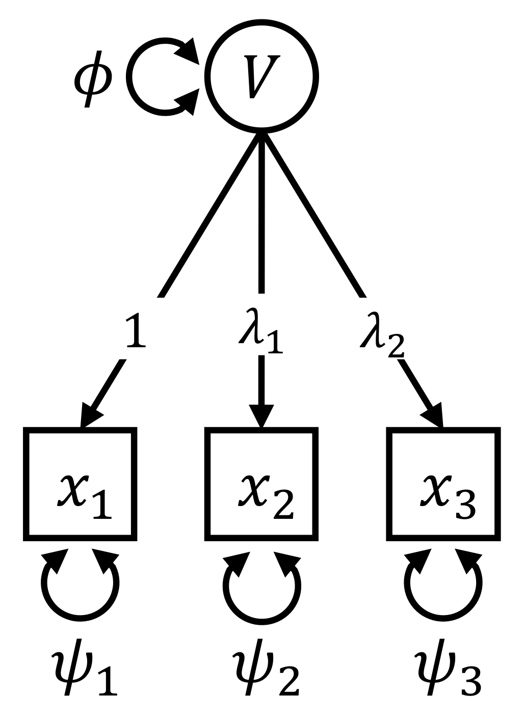
6.3. Simulation III: Group Difference in the Measurement Part

In Simulation III, we introduced heterogeneity to the measurement part of the model shown in Figure 7 by letting the factor loading λ vary between two groups. The regression parameter β was constant and was set to 0.5. IPC regression was provided with a grouping variable to predict the group difference. As a reference, we compared the performance of IPC regression with MGSEMs. The power to detect group differences of MGSEMs was assessed by performing likelihood-ratio tests between a MGSEM where λ was allowed to vary between groups and a single-group SEM where λ was constrained to be equal between groups. The remaining parameters of the MGSEMs were constrained to be equal between groups. The following simulation conditions were investigated:
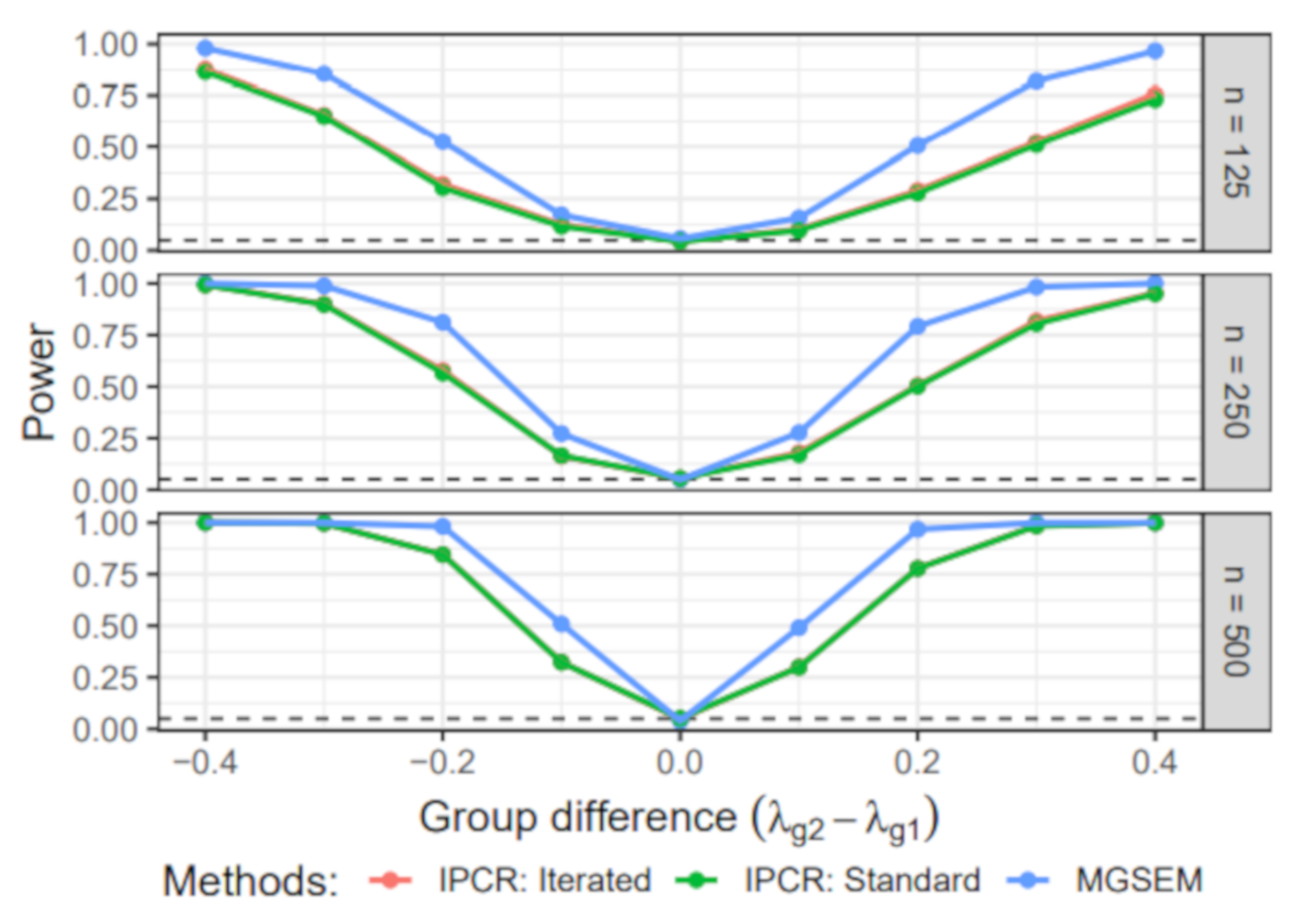
  • Group-specific value of λ: The value of the factor loading in the first group λ g 1 was set to 1. For the second group, the value of λ g 2 varied across 0.6, 0.7, 0.8, 0.9, 1, 1.1, 1.2, 1.3, and 1.4.
  • Sample size: The sample size per group n was either 125, 250, 500. Therefore, the total sample size N was 250, 500, or 1000.

6.3.1. Power

Figure 8 shows the power of standard and iterated IPC regression and the MGSEMs to detect the differences in the factor loading λ . The power of standard and iterated IPC regression was nearly identical, resulting in overlapping lines. As expected, the power of all methods grew substantively with the sample size and the size of the group differences. MGSEMs were consistently more powerful than the IPC regression methods in detecting the group difference. For medium-sized group differences, when λ g 2 was either 0.8 or 1.2, we found MGSEMs on average to outperform the IPC regression methods by roughly 21 percentage points. When λ g 2 = 1 , the factor loading was identical in both groups, resulting in a homogeneous sample. In this case, the proportions of significant tests approached the significance level of 5% for all methods.

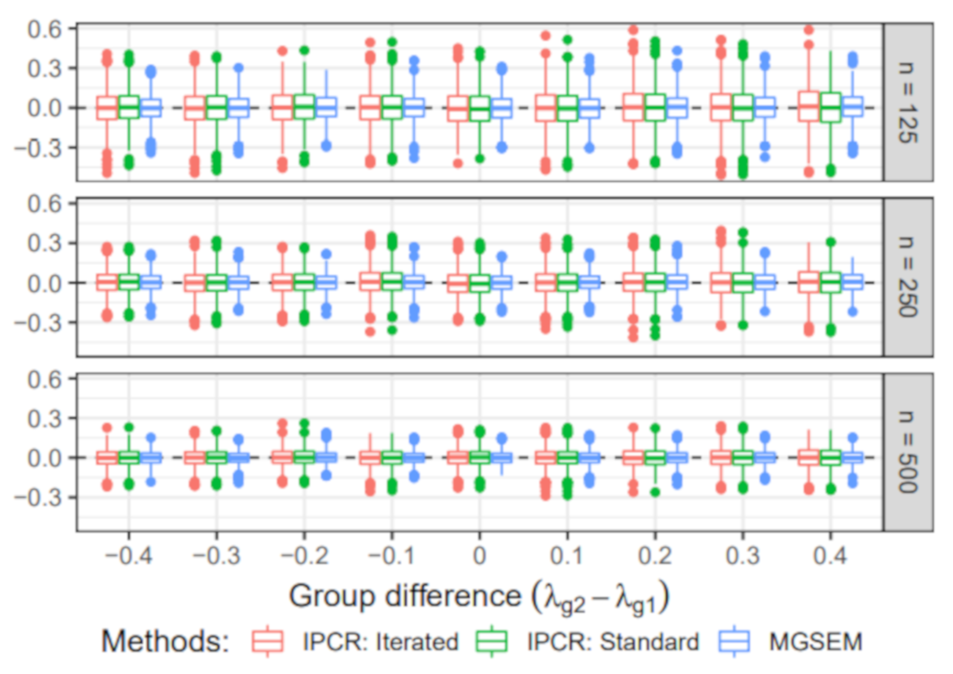
6.3.2. Estimated Group Difference

Figure 9 presents boxplots of the bias of the estimated group difference in the factor loading, provided by standard and iterated IPC regression and MGSEMs. All methods produced nearly unbiased estimates. The estimates of the group difference provided by MGSEMs exhibited less variability than the IPC regression estimates in all experimental conditions. In terms of the root mean squared error (RMSE) averaged over the two group-specific estimates of the factor loading, MGSEMs (RMSE: 0.067) were marginally more accurate than standard (RMSE: 0.076) and iterated (RMSE: 0.077) IPC regression.

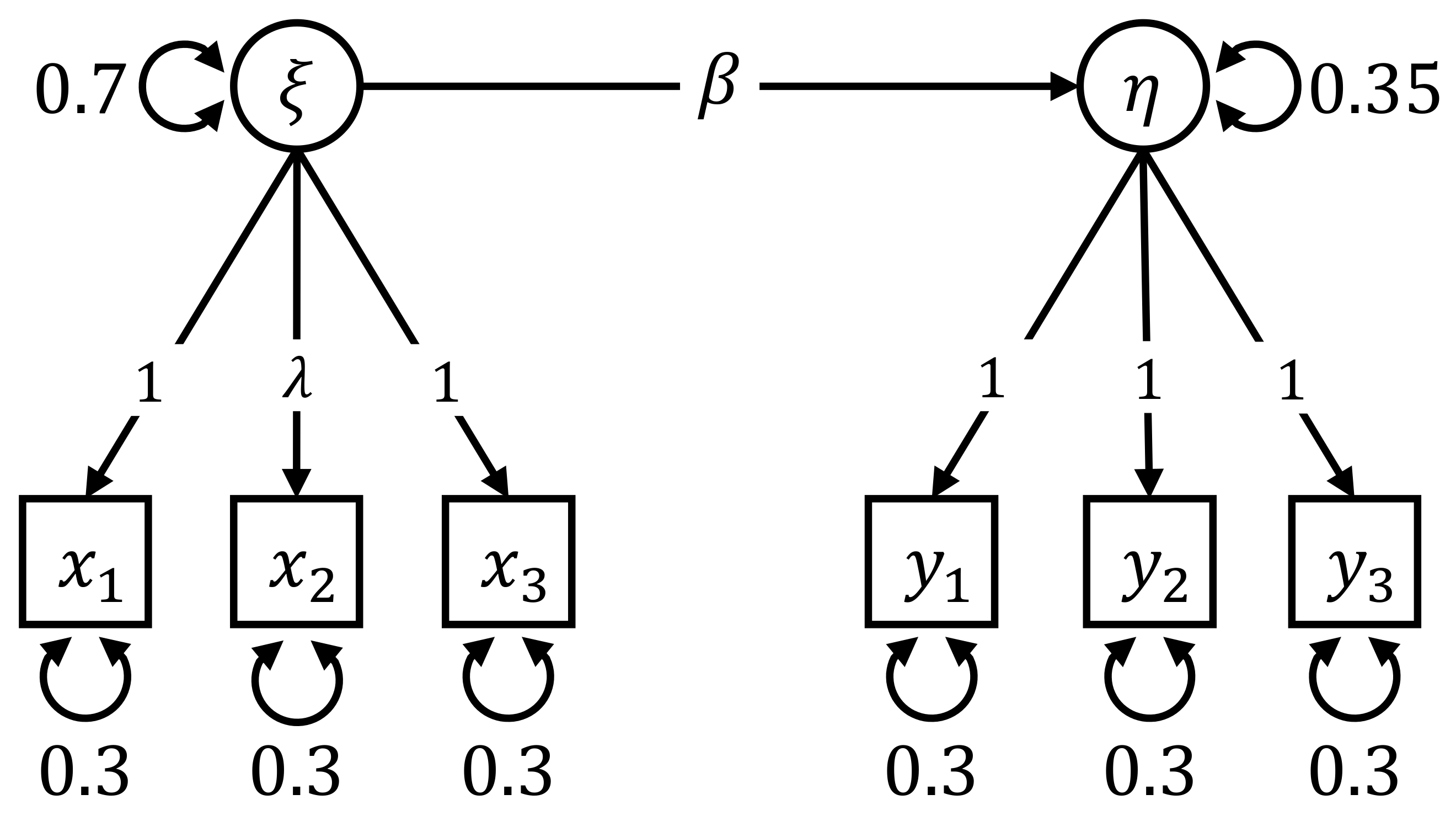
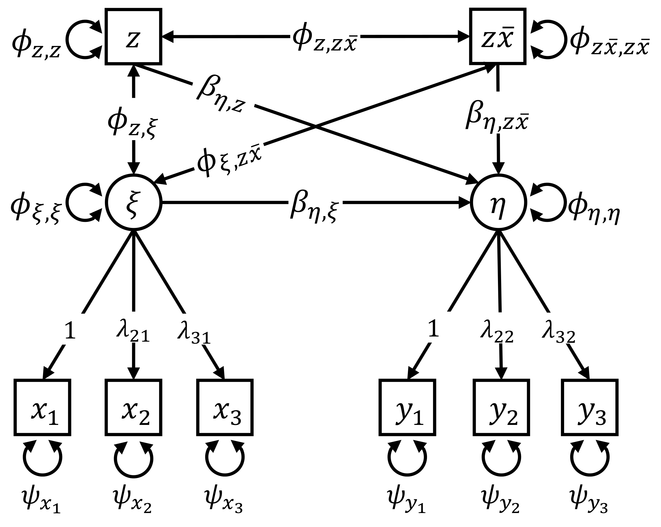
6.4. Simulation IV: Individual Differences in the Structural Part

In Simulation IV, we compared the performance of standard and iterated IPC regression to a SEMs with an interaction term. The data were generated by letting the regression parameter β vary across individuals and fixing the factor loading λ at 1. More specifically, the individual values of β were a linear function of a standard normally distributed covariate z:
β i = 0.5 + γ z i
The value of the coefficient γ determined the relationship between covariate and regression parameter and was of primary interest in this simulation. We investigated the following simulation conditions:
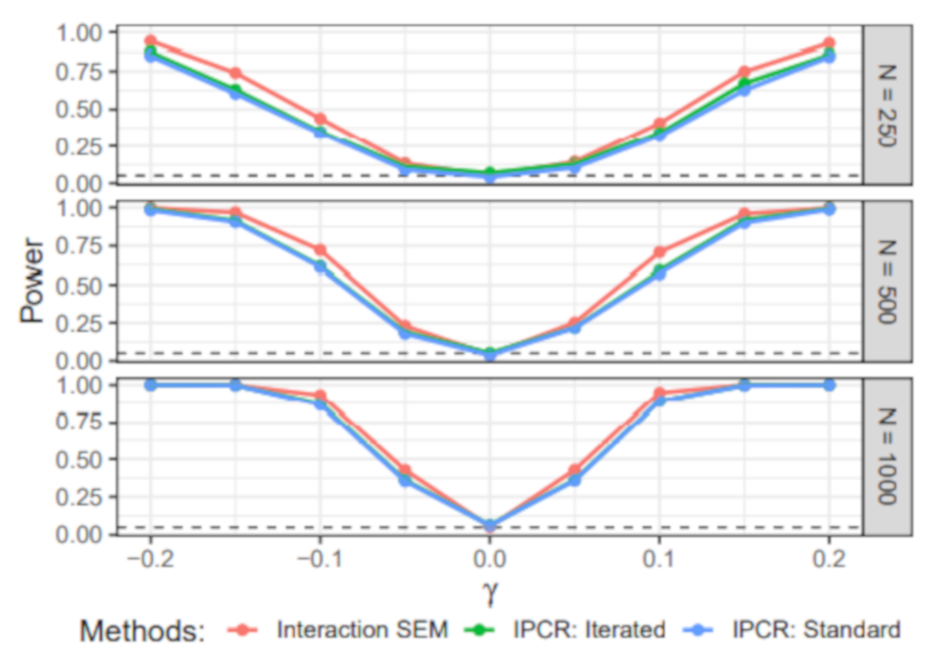
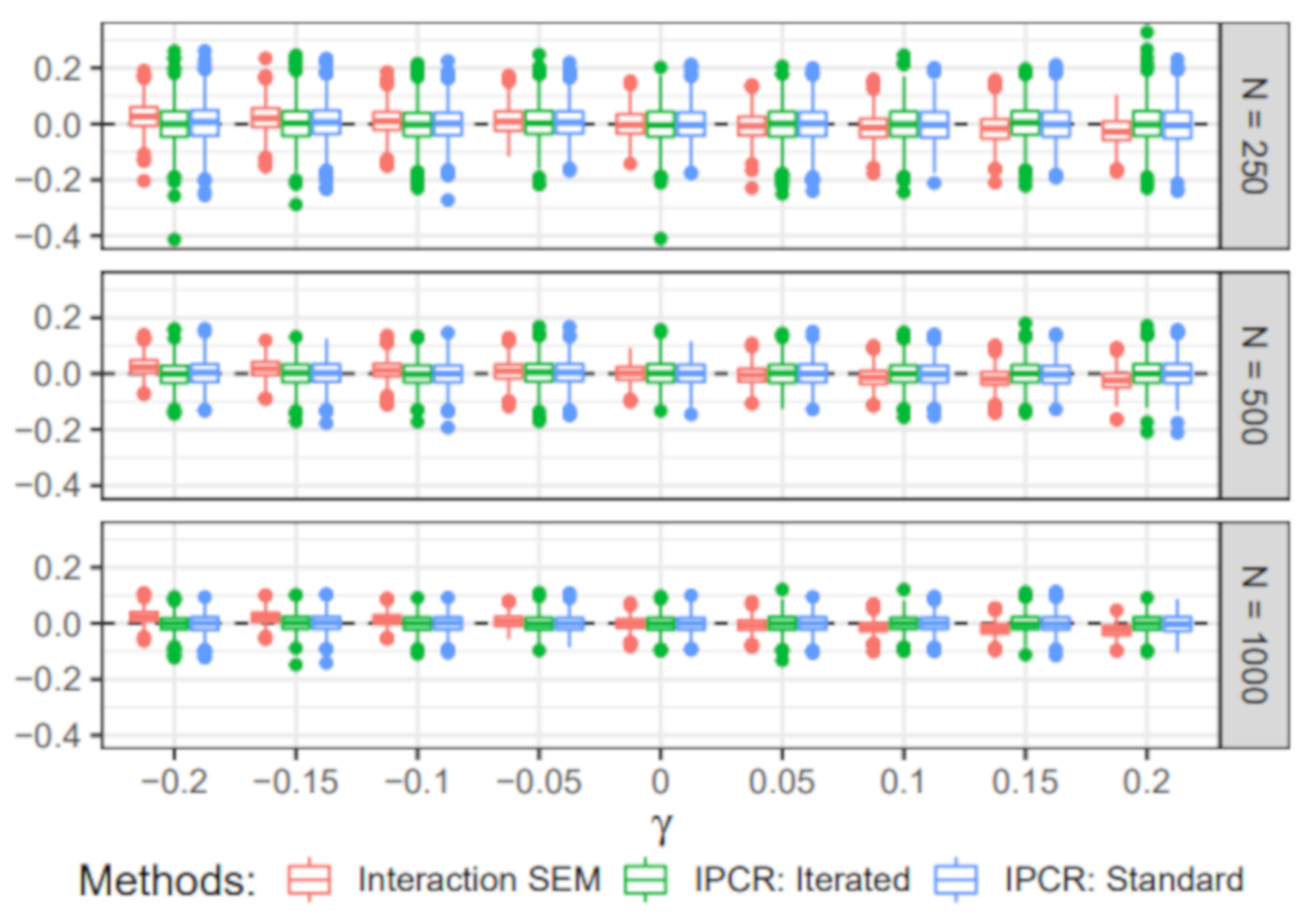
  • Value of γ: The dependency of the individual regression parameter values on the covariate was either −0.2, −0.15, −0.1, −0.05, 0, 0.05, 0.1, 0.15, or 0.2. Note that the zero condition corresponds to a homogeneous sample with a constant regression parameter β .
  • Sample size (N): The simulated samples contained either 250, 500, or 1000 individuals.
There are several ways to specify SEMs with interactions (see [10] for an overview). Following Marsh et al. [35], we contrasted IPC regression with a SEM containing a product term consisting of the indicators of the exogenous latent variable ξ and the covariate z. We used a parcel of the indicators x 1 , x 2 , and x 3 to create this product term, which we denote with z x ¯ . Note that x ¯ refers to the row-wise means and not the mean of a single variable. We also added the covariate to the model and specified a main effect of the covariate on the endogenous latent variable η . Moreover, we let all exogenous predictor variables co-vary. Finally, to avoid having to specify a mean structure, we used double-mean centering (see [36]); that is, we centered all manifest variables, computed the product term using the centered variables, and then centered the product term again. A path diagram of the interaction model is shown in Figure 10. The direct effect of the product term on the endogenous variable (i.e., the regression parameter β η , z x ¯ ) is an estimate of the coefficient γ in Equation (16). We assessed the power of the SEMs with a product term by testing the hypothesis β η , z x ¯ = 0 via z-tests.

6.4.1. Power

Figure 11 presents the observed power of the IPC regression methods and the interaction SEMs to detect that the regression parameter β depended on the covariate z. As in Simulation II, the power of standard and iterated IPC regression was nearly the same. The SEMs with the product term were slightly more powerful than the IPC regression methods. The largest difference in power was found when the sample consisted of 500 individuals and the absolute value of the coefficient γ was 0.1. Under this condition, the SEMs with a product term outperformed the IPC regression methods by approximately 15 percentage points. For γ = 0 , when the regression parameter β did not depend on the covariate z, the proportions of significant tests of all methods approached the significance level of 5%.

6.4.2. Estimated Interaction

Figure 12 shows boxplots with the bias of the estimates of the coefficient γ provided by standard and iterated IPC regression and the SEMs with a product term. SEMs with a product term underestimated the absolute value of the dependency slightly. In comparison, IPC regression yielded mostly unbiased but also more volatile estimates. Especially in smaller samples with 250 observations, iterated IPC regression produced some outliers that were not found in the estimates provided by standard IPC regression. In terms of RMSE averaged over all simulation conditions, standard (RMSE: 0.051) and iterated (RMSE: 0.051) IPC regression were marginally outperformed by SEMs with a product term (RMSE: 0.042).
Additional information about the convergence of the iterated IPC regression algorithm is given in Appendix A.2.

7. Discussion

The present study showed how differences in model parameters can be predicted with IPC regression using the ipcr package. We showcased the functionality of the ipcr package using a classic data set and provided detailed R code. We expanded upon earlier research about predicting parameter differences in SEMs and demonstrated that IPC regression can also predict parameter differences in linear regression models. Moreover, we presented novel simulation results that illuminated the method’s performance for linear regression models and contrasted it with SEMs with an interaction term.
We see IPC regression primarily as a diagnostic tool that indicates whether there is any predictive potential for parameter heterogeneity in a set of covariates and provides researchers with hints on how these covariates can be integrated into their models. As such, IPC regression offers some advantages compared to other procedures for exploring heterogeneity with covariates. One of these advantages is the flexibility of the method: IPC regression allows researchers to investigate all types of model parameters. We demonstrated this flexibility by predicting group differences in the error variance of a linear regression model. Another merit of IPC regression is its simplicity. Especially for model classes where model specification and estimation can become complicated such as SEMs, researchers can obtain results much quicker with IPC regression via a single call of the ipcr() function than, for instance, from specifying and estimating MGSEMs and SEMs with interaction terms. One can also argue that this simplicity makes IPC regression less prone to specification errors and may prove useful if a complex model is hard to estimate. Finally, IPC regression can guide the selection of important covariates among a larger set of covariates, particularly in combination with LASSO regularization as implemented in the ipcr package.
The question remains as to how we can best translate the results of IPC regression into an improved parametric model. A key problem of data-driven methods like IPC regression is their susceptibility to capitalize on chance, that is, to overfit to noise in the data (see [37,38] for a discussion of the problem). In other words, IPC regression may indicate model modifications that increase the model’s fit in the sample at hand but generalize poorly to new data. The risk of overfitting rises with the complexity of the model and the number of covariates. For example, given a model with 10 parameters and a set of 10 covariates, IPC regression will produce 100 IPC regression estimates with associated p-values. Using the conventional 5% level of significance and assuming homogeneous data (i.e., no parameter differences at all), one would expect to 5 five false-positive effects of a covariate on a model parameter on average. We recommend three different strategies to minimize the risk of overfitting the model. First, adopting a machine learning perspective, we encourage researchers to apply regularized IPC regression, which penalizes each regression for model complexity. Second, if the sample size is sufficiently large, one should additionally split the sample into a training and a test data set. The training data set is used for model estimation with IPC regression. After modifying the model following the results of IPC regression, the fit of the new augmented model is then independently evaluated in the test data set. Third, we suggest considering the estimated change in model parameters in addition to p-values to determine how to modify a given theory-based model. For instance, a statistically significant group difference in a parameter may be just too small to be of scientific interest and would not necessarily warrant model modification. In most cases, such thresholds for scientific relevancy will be different for different types of parameters. Most likely, heterogeneity in nuisance parameters such as an error variance needs to be much more pronounced than heterogeneity in a regression parameter central to one’s inquiry to justify a model modification.
The results of our simulations were overall promising. In line with previous simulation studies reported by Oberski [11] and Arnold et al. [12], we found that IPC regression provided adequate control of type I errors under the null hypothesis of homogeneous parameters. Moreover, we found little differences in terms of bias and variance of the estimates provided by IPC regression and MGSEMs. However, as in the previous simulation studies, IPC regression was consistently less powerful in detecting parameter heterogeneity than MGSEMs. We expanded upon previous studies that only discussed IPC regression for SEMs and predicted a group difference in the error variance of a linear regression model. The estimates of the group differences were slightly biased. In another simulation study, we compared IPC regression to SEMs with a product interaction term suggested by Marsh et al. [10]. Interestingly, IPC regression was more accurate but less precise than SEMs with an interaction term and exhibited a lower power. As part of our simulation studies, we also compared standard IPC regression with iterated IPC regression. Iterated IPC regression was suggested by Arnold et al. [12] as an unbiased alternative to standard IPC regression. Unfortunately, these comparisons were limited to SEMs as iterated IPC regression has not yet been implemented for other model classes. Both IPC regression methods yielded almost identical results in terms of power and bias. However, iterated IPC regression showed some cases of non-convergence, especially in smaller samples and when provided with continuous covariates. Furthermore, the type I error rate of iterated IPC regression was marginally larger than the significance level in smaller samples. Similar performance of the IPC regression methods was to be expected because the parameter differences tested were too small to bias standard IPC regression.
Although the ipcr package makes performing IPC regression for various parametric models straightforward in most situations, it is still under ongoing development, and we would like to note some of its current limitations. The biased estimates obtained for the linear regression model underline the need to generalize the iterated IPC regression algorithm and develop a version for regression models. Moreover, the sometimes poor convergence rate of iterated IPC regression highlights the necessity for an improved algorithm that is more reliable in smaller samples and when provided with continuous covariates. Another limitation is that IPC regression currently requires complete data sets without missing values. Especially for researchers working with SEMs who routinely employ full information maximum likelihood to deal with missingness, this limitation might be an issue. We plan to implement support for SEMs fitted on incomplete data in the future. In the meantime, we suggest using an imputation technique such as multiple imputation as a workaround [27,28]. Finally, even though the combination of IPC regression and regularization seems like a natural fit to handle larger sets of covariates, more research is needed to understand this interplay better and determine better default settings.
IPC regression may not always be the best choice for exploring parameter heterogeneity with covariates. Besides adding covariates directly to the model, other techniques are available for testing and estimating the effects of covariates. If the sample is clustered into known groups, mixed-effects or multilevel models (e.g., [39,40]) are an obvious alternative and allow parameters to vary across groups. Unlike IPC regression, the use of mixed-effects models is usually motivated by a prior belief that certain data segments differ. In contrast, IPC regression is a more exploratory or data-driven procedure to identify potentially important covariates. Further, IPC regression does not rely on a clustered data structure. Of course, IPC regression can also be used to study heterogeneity in mixed-effects models. Other methods for exploring parameter heterogeneity are structural change tests (e.g., [16,18]). These tests have been recently introduced to psychometrics and are applied to discover parameter differences with respect to a covariate [19]. Especially if one wants to explore the effect of ordinal covariates, which can be hard to incorporate in the regression framework, structural change tests may be a well-suited alternative (see [20]). However, unlike IPC regression, structural change tests are limited to testing if a parameter changes but do not estimate how it changes with respect to a covariate. Another established approach to investigate heterogeneity with covariates are model-based recursive partitioning techniques (e.g., [41,42]). These methods divide a data set into homogeneous subgroups by finding covariates that predict parameter differences. For SEMs, model-based recursive partitioning was popularized as SEM trees and gained attention in the past years [43,44,45]. Finally, it is important to note that the performance of IPC regression depends primarily on the available covariates. If there are parameter differences, but these differences are unrelated to the covariates, IPC regression will fail to detect them. That is, covariates need to be sufficiently informative and reliable to be usable in the context of IPC regression. Consequently, IPC regression is not a global test of heterogeneity. Methods such as finite mixture models (e.g., [46,47,48]) that do not depend on covariates provide a more thorough test of parameter homogeneity than IPC regression.
Having these alternatives to IPC regression and limitations of the ipcr package in mind, we believe that IPC regression can be applied in many situations to uncover heterogeneity and gross model misspecification. Furthermore, in many cases in which additional covariates are available, it makes sense to run IPC regression as part of exploration and model checking procedures. Note that IPC regression should then be labeled as exploratory analyses and run only after all confirmatory actions were performed.

Supplementary Materials

The following are available at https://osf.io/p5xrk.

Author Contributions

Conceptualization, M.A., A.M.B. and M.C.V.; methodology, M.A.; software, M.A.; validation, M.A.; formal analysis, M.A.; investigation, M.A.; resources, A.M.B.; data curation, M.A.; writing—original draft preparation, M.A.; writing—review and editing, M.A., A.M.B. and M.C.V.; visualization, M.A.; supervision, A.M.B. and M.C.V.; project administration, M.A. All authors have read and agreed to the published version of the manuscript.

Funding

This research received no external funding.

Institutional Review Board Statement

Not applicable.

Informed Consent Statement

Not applicable.

Data Availability Statement

The simulated data presented in this study can be found in the following online repository: https://osf.io/p5xrk (accessed on 5 August 2021). The developmental snapshot of the ipcr package can be downloaded here: https://github.com/manuelarnold/ipcr/commit/d4132c73b0e05ced1da6be71119d846424a1a3d6 (accessed on 5 August 2021).

Conflicts of Interest

The authors declare no conflict of interest.

Appendix A. Convergence of Iterated IPC Regression

The iterated IPC algorithm was not always able to find a satisfactory solution. We counted all simulation trials in which the algorithm did not converge after 50 iterations or aborted prematurely as a non-converged trial. In the following, we report the percentages of non-converged trials for Simulation II and IV. All attempts converged in Simulation III. Iterated IPC regression was not evaluated in Simulation I as it has not yet been implemented for linear regression models.

Appendix A.1. Simulation II

Table A1 presents the percentages of non-converged trials for continuous covariates. The instability of the iterated IPC regression algorithm was driven by the sample size and the number of continuous covariates. Smaller samples and more continuous covariates led to a larger number of non-converged trials. However, when provided with dummy variables, the iterated IPC algorithm was much more stable, and there were only four instances of non-convergence for smaller samples with 250 individuals and three covariates.
Table A1. Non-Convergence of the Iterated IPC Regression Algorithm.
   NNumber of CovariatesNC a
   25013.10
   50010.20
   100010.00
   25029.90
   50020.60
   100020.00
   250324.40
   50033.20
   100030.00
a Percentages of the non-converged simulation trials.

Appendix A.2. Simulation IV

Table A2 summarizes the percentages of trials in which the iterated IPC regression algorithm did not converge, separated for different sample sizes. Convergence problems were mainly limited to smaller samples with 250 individuals, whereas iterated IPC regression found a solution almost every time in larger samples.
Table A2. Non-Convergence of the Iterated IPC Regression Algorithm.
       NNC a
       2504.2
       5000.3
       10000
a Percentages of the non-converged simulation trials.

References

  1. Lindenberger, U. Human cognitive aging: Corriger la fortune? Science 2014, 346, 572–578. [Google Scholar] [CrossRef]
  2. Kuehner, C. Why is depression more common among women than among men? Lancet Psychiatry 2017, 4, 146–158. [Google Scholar] [CrossRef]
  3. Jedidi, K.; Jagpal, H.S.; DeSarbo, W.S. Finite-Mixture Structural Equation Models for Response-Based Segmentation and Unobserved Heterogeneity. Mark. Sci. 1997, 16, 39–59. [Google Scholar] [CrossRef]
  4. Becker, J.M.; Rai, A.; Ringle, C.M.; Völckner, F. Discovering Unobserved Heterogeneity in Structural Equation Models to Avert Validity Threats. MIS Q. 2013, 37, 665–694. [Google Scholar] [CrossRef] [Green Version]
  5. R Core Team. R: A Language and Environment for Statistical Computing; R Foundation for Statistical Computing: Vienna, Austria, 2020. [Google Scholar]
  6. Bates, D.; Mächler, M.; Bolker, B.; Walker, S. Fitting Linear Mixed-Effects Models Using lme4. J. Stat. Softw. 2015, 67. [Google Scholar] [CrossRef]
  7. Bollen, K.A. Structural Equations with Latent Variables; John Wiley & Sons, Inc.: Hoboken, NJ, USA, 1989. [Google Scholar] [CrossRef]
  8. Kline, R.B. Principles and Practice of Structural Equation Modeling, 4th ed.; Methodology in the Social Sciences; The Guilford Press: New York, NY, USA; London, UK, 2016. [Google Scholar]
  9. Sörbom, D. A general method for studying differences in factor means and factor structure between groups. Br. J. Math. Stat. Psychol. 1974, 27, 229–239. [Google Scholar] [CrossRef]
  10. Marsh, H.W.; Wen, Z.; Nagengast, B.; Hau, K.-T. Structural equation models of latent interaction. In Handbook of Structural Equation Modeling; Hoyle, R.H., Ed.; Guilford Press: New York, NY, USA, 2012; pp. 436–458. [Google Scholar]
  11. Oberski, D.L. A Flexible Method to Explain Differences in Structural Equation Model Parameters over Subgroups. Available online: http://daob.nl/wp-content/uploads/2013/06/SEM-IPC-manuscript-new.pdf (accessed on 5 August 2021).
  12. Arnold, M.; Oberski, D.L.; Brandmaier, A.M.; Voelkle, M.C. Identifying Heterogeneity in Dynamic Panel Models with Individual Parameter Contribution Regression. Struct. Equ. Model. Multidiscip. J. 2020, 27, 613–628. [Google Scholar] [CrossRef] [Green Version]
  13. Sörbom, D. Model modification. Psychometrika 1989, 54, 371–384. [Google Scholar] [CrossRef]
  14. Saris, W.E.; Satorra, A.; Sorbom, D. The Detection and Correction of Specification Errors in Structural Equation Models. Sociol. Methodol. 1987, 17, 105. [Google Scholar] [CrossRef]
  15. Saris, W.E.; Satorra, A.; van der Veld, W.M. Testing Structural Equation Models or Detection of Misspecifications? Struct. Equ. Model. Multidiscip. J. 2009, 16, 561–582. [Google Scholar] [CrossRef]
  16. Hjort, N.L.; Koning, A. Tests For Constancy Of Model Parameters Over Time. J. Nonparametric Stat. 2002, 14, 113–132. [Google Scholar] [CrossRef]
  17. Zeileis, A.; Hornik, K. Generalized M-fluctuation tests for parameter instability. Stat. Neerl. 2007, 61, 488–508. [Google Scholar] [CrossRef]
  18. Andrews, D.W.K. Tests for Parameter Instability and Structural Change With Unknown Change Point. Econometrica 1993, 61, 821. [Google Scholar] [CrossRef] [Green Version]
  19. Merkle, E.C.; Zeileis, A. Tests of measurement invariance without subgroups: A generalization of classical methods. Psychometrika 2013, 78, 59–82. [Google Scholar] [CrossRef]
  20. Merkle, E.C.; Fan, J.; Zeileis, A. Testing for measurement invariance with respect to an ordinal variable. Psychometrika 2014, 79, 569–584. [Google Scholar] [CrossRef] [Green Version]
  21. Rosseel, Y. Lavaan: An R Package for Structural Equation Modeling. J. Stat. Softw. 2012, 48, 1–36. [Google Scholar] [CrossRef] [Green Version]
  22. Stefanski, L.A.; Boos, D.D. The Calculus of M-Estimation. Am. Stat. 2002, 56, 29–38. [Google Scholar] [CrossRef]
  23. Zeileis, A.; Köll, S.; Graham, N. Various Versatile Variances: An Object-Oriented Implementation of Clustered Covariances in R. J. Stat. Softw. 2020, 95, 1–36. [Google Scholar] [CrossRef]
  24. Neale, M.C.; Hunter, M.D.; Pritikin, J.N.; Zahery, M.; Brick, T.R.; Kirkpatrick, R.M.; Estabrook, R.; Bates, T.C.; Maes, H.H.; Boker, S.M. OpenMx 2.0: Extended Structural Equation and Statistical Modeling. Psychometrika 2016, 81, 535–549. [Google Scholar] [CrossRef] [PubMed]
  25. Wang, T.; Strobl, C.; Zeileis, A.; Merkle, E.C. Score-Based Tests of Differential Item Functioning via Pairwise Maximum Likelihood Estimation. Psychometrika 2018, 83, 132–155. [Google Scholar] [CrossRef]
  26. Wickham, H.; Hester, J.; Chang, W. Devtools: Tools to Make Devoloping R Packages Easier. [Computer software manual]. (R package version 2.3.2). 2020. Available online: https://cran.r-project.org/web/packages/devtools/ (accessed on 6 August 2021).
  27. Van Buuren, S. Flexible Imputation of Missing Data, 2nd ed.; CRC Press: Boca Raton, FL, USA; London, UK; New York, NY, USA, 2018. [Google Scholar]
  28. Meinfelder, F. Multiple Imputation: An attempt to retell the evolutionary process. AStA Wirtsch. Sozialstat. Arch. 2014, 8, 249–267. [Google Scholar] [CrossRef] [Green Version]
  29. Cohen, J.; Cohen, P.; West, S.G.; Aiken, L.S. Applied Multiple Regression/Correlation Analysis for the Behavioral Sciences, 3rd ed.; Routledge Taylor & Francis Group: New York, NY, USA; London, UK; Mahwah, NJ, USA, 2003. [Google Scholar]
  30. Tibshirani, R. Regression Shrinkage and Selection Via the Lasso. J. R. Stat. Soc. Ser. B 1996, 58, 267–288. [Google Scholar] [CrossRef]
  31. Tibshirani, R. Regression shrinkage and selection via the lasso: A retrospective. J. R. Stat. Soc. Ser. B 2011, 73, 273–282. [Google Scholar] [CrossRef]
  32. Shmueli, G. To Explain or to Predict? Stat. Sci. 2010, 25, 289–310. [Google Scholar] [CrossRef]
  33. Friedman, J.; Hastie, T.; Tibshirani, R. Regularization Paths for Generalized Linear Models via Coordinate Descent. J. Stat. Softw. 2010, 33, 1. [Google Scholar] [CrossRef] [Green Version]
  34. Boynton, P.M.; Wood, G.W.; Greenhalgh, T. Reaching beyond the white middle classes. BMJ 2004, 328, 1433–1436. [Google Scholar] [CrossRef] [Green Version]
  35. Marsh, H.W.; Wen, Z.; Hau, K.T. Structural equation models of latent interactions: Evaluation of alternative estimation strategies and indicator construction. Psychol. Methods 2004, 9, 275–300. [Google Scholar] [CrossRef]
  36. Lin, G.C.; Wen, Z.; Marsh, H.; Lin, H.S. Structural Equation Models of Latent Interactions: Clarification of Orthogonalizing and Double-Mean-Centering Strategies. Struct. Equ. Model. Multidiscip. J. 2010, 17, 374–391. [Google Scholar] [CrossRef]
  37. MacCallum, R.C.; Roznowski, M.; Necowitz, L.B. Model modifications in covariance structure analysis: The problem of capitalization on chance. Psychol. Bull. 1992, 111, 490–504. [Google Scholar] [CrossRef]
  38. Yarkoni, T.; Westfall, J. Choosing Prediction Over Explanation in Psychology: Lessons From Machine Learning. Perspect. Psychol. Sci. J. Assoc. Psychol. Sci. 2017, 12, 1100–1122. [Google Scholar] [CrossRef]
  39. Raudenbush, S.W.; Bryk, A.S. Hierarchical linear models: Applications and data analysis methods. In Advanced Quantitative Techniques in the Social Sciences, 2nd ed.; SAGE Publications: Thousand Oaks, CA, USA, 2002; Volume 1. [Google Scholar]
  40. Singer, J.D.; Willett, J.B. Applied Longitudinal Data Analysis: Modeling Change and Event Occurrence; Oxford University Press: Oxford, UK, 2003. [Google Scholar]
  41. Zeileis, A.; Hothorn, T.; Hornik, K. Model-Based Recursive Partitioning. J. Comput. Graph. Stat. 2008, 17, 492–514. [Google Scholar] [CrossRef] [Green Version]
  42. Strobl, C.; Malley, J.; Tutz, G. An introduction to recursive partitioning: Rationale, application, and characteristics of classification and regression trees, bagging, and random forests. Psychol. Methods 2009, 14, 323–348. [Google Scholar] [CrossRef] [Green Version]
  43. Brandmaier, A.M.; von Oertzen, T.; McArdle, J.J.; Lindenberger, U. Structural equation model trees. Psychol. Methods 2013, 18, 71–86. [Google Scholar] [CrossRef] [Green Version]
  44. Brandmaier, A.M.; Prindle, J.J.; McArdle, J.J.; Lindenberger, U. Theory-guided exploration with structural equation model forests. Psychol. Methods 2016, 21, 566–582. [Google Scholar] [CrossRef] [PubMed] [Green Version]
  45. Arnold, M.; Voelkle, M.C.; Brandmaier, A.M. Score-Guided Structural Equation Model Trees. Front. Psychol. 2021, 11, 3913. [Google Scholar] [CrossRef] [PubMed]
  46. Lubke, G.H.; Muthén, B. Investigating population heterogeneity with factor mixture models. Psychol. Methods 2005, 10, 21–39. [Google Scholar] [CrossRef] [Green Version]
  47. Muthén, B.; Shedden, K. Finite mixture modeling with mixture outcomes using the EM algorithm. Biometrics 1999, 55, 463–469. [Google Scholar] [CrossRef]
  48. McLachlan, G.J.; Peel, D. Finite Mixture Models; Wiley Series in Probability and Statistics Applied Probability and Statistics Section; Wiley: New York, NY, USA, 2000. [Google Scholar]
Figure 1. The three steps of IPC regression. Panel A shows the model under investigation. It is not necessary to include any covariates in the model. Panel B visualizes the structure of the new data matrix containing the IPCs. Panel C shows the three IPC regression equations for the respective model parameters. Note that we model the IPCs to each of the three model parameters in a separate regression model.
Psych 03 00027 g001
Figure 3. Correlations between covariates (x-axis) and the IPCs of the model parameters (y-axis) obtained with plot(ipcr_visual, print_corr = TRUE). Parameter names are given in lavaan syntax.
Psych 03 00027 g003
Figure 4. Estimated conditional differences in the factor loading of the indicator x3. Left plot: IPCs to the factor loading are plotted on the students’ age in months. The solid blue line marks the estimated factor loading as a function of months when all other covariates are zero. The dashed blue lines represent the upper and lower limit of the 95% pointwise confidence bands. Right plot: IPCs to the factor loading are plotted on the students’ gender. The big dots mark the estimated factor loadings for girls and boys when all other covariates are zero. The error bars indicate the 95% confidence intervals of the estimated gender-specific factor loading.
Psych 03 00027 g004
Figure 5. The power of IPC regression to detect a group difference in the error variance σ 2 . The dashed line marks a power of 5%.
Psych 03 00027 g005
Figure 6. Boxplots with the bias of the estimated group difference in the error variance σ 2 .
Psych 03 00027 g006
Figure 7. Path diagram of the simulation model. The factor loading λ varied between two groups in Simulation III and the regression parameter β differed across individuals in Simulation IV.
Psych 03 00027 g007
Figure 8. The power of standard and iterated IPC regression and MGSEMs to detect a group difference in the factor loading λ . The dashed line marks a power of 5%.
Psych 03 00027 g008
Figure 9. Boxplots with the bias of the estimated group difference in the factor loading λ (y-axis) for different true group differences and sample sizes.
Psych 03 00027 g009
Figure 10. Path diagram of the interaction model with a product term.
Psych 03 00027 g010
Figure 11. The power of standard and iterated IPC regression and SEMs with a product term to detect the dependency of the regression parameter β on the covariate z. The dashed line marks a power of 5%.
Psych 03 00027 g011
Figure 12. Boxplots with the bias of the estimates of the dependency γ (y-axis) for different values of γ and sample sizes.
Psych 03 00027 g012
Table 1. Selected variables from the HolzingerSwineford1939 data set.
Variable NameDescriptionLevel of Measurement
Model data:
x1Visual perceptionInterval ( M = 4.94 , S D = 1.17 )
x2CubesInterval ( M = 6.09 , S D = 1.18 )
x3LozengesInterval ( M = 2.25 , S D = 1.13 )
Covariates:
sexGenderNominal (48.3% female, 51.7% male)
ageyrAge, year partInterval ( M = 13.00 , S D = 1.05 )
agemoAge, month partInterval ( M = 5.38 , S D = 3.46 )
schoolSchool (Pasteur or Grant-White)Nominal (52% Pasteur, 48% Grant-White)
gradeGradeOrdinal (52.3% grade 7, 47.7% grade 8)
Note: M: mean, S D : standard deviation.
Publisher’s Note: MDPI stays neutral with regard to jurisdictional claims in published maps and institutional affiliations.

