
Automated Test Assembly in R: The eatATA Package


Abstract
:1. Theoretical Background
2. eatATA
2.1. Work Flow
- (1)
- Item Pool: A data.frame including all information on the item pool is loaded or created. If the items have already been calibrated (e.g., based on data from a pilot study) this will include the calibrated item parameters.
- (2)
- Test Specifications: Usually a combination of: (a) Typically one objective and (b) multiple constraints.
- (a)
- Objective Function: Usually a single object corresponding to the optimization goal, created via one of the objective function functions. This refers to a test specification where we have no absolute criterion, but where we want to minimize or maximize something.
- (b)
- Further Constraints: Further constraint objects, created using various constraint functions. These refer to test specifications with a fixed value or an upper and/or lower bound.
- (3)
- Solver Call: The useSolver() function is called using the constraint objects to find an optimal solution.
- (4)
- Solution Processing: The solution can be inspected using the inspectSolution() and appendSolution() functions.
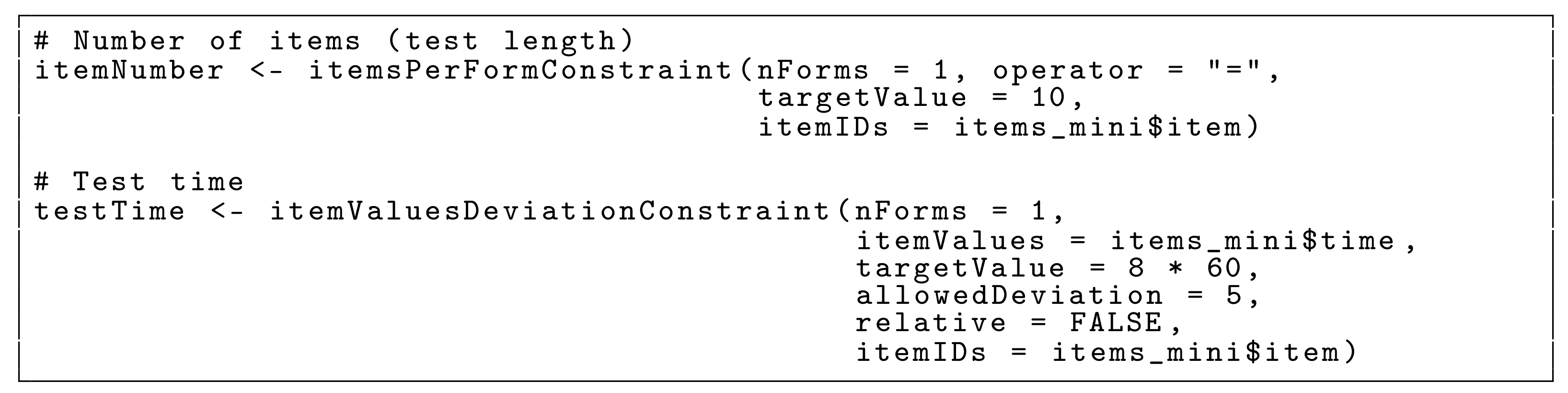
2.2. Minimal Example
- (1)
- Item Pool
- (2a)
- Objective Function
- (2b)
- Constraints
- (3)
- Solver Call
- (4)
- Solution Processing
3. Use Cases
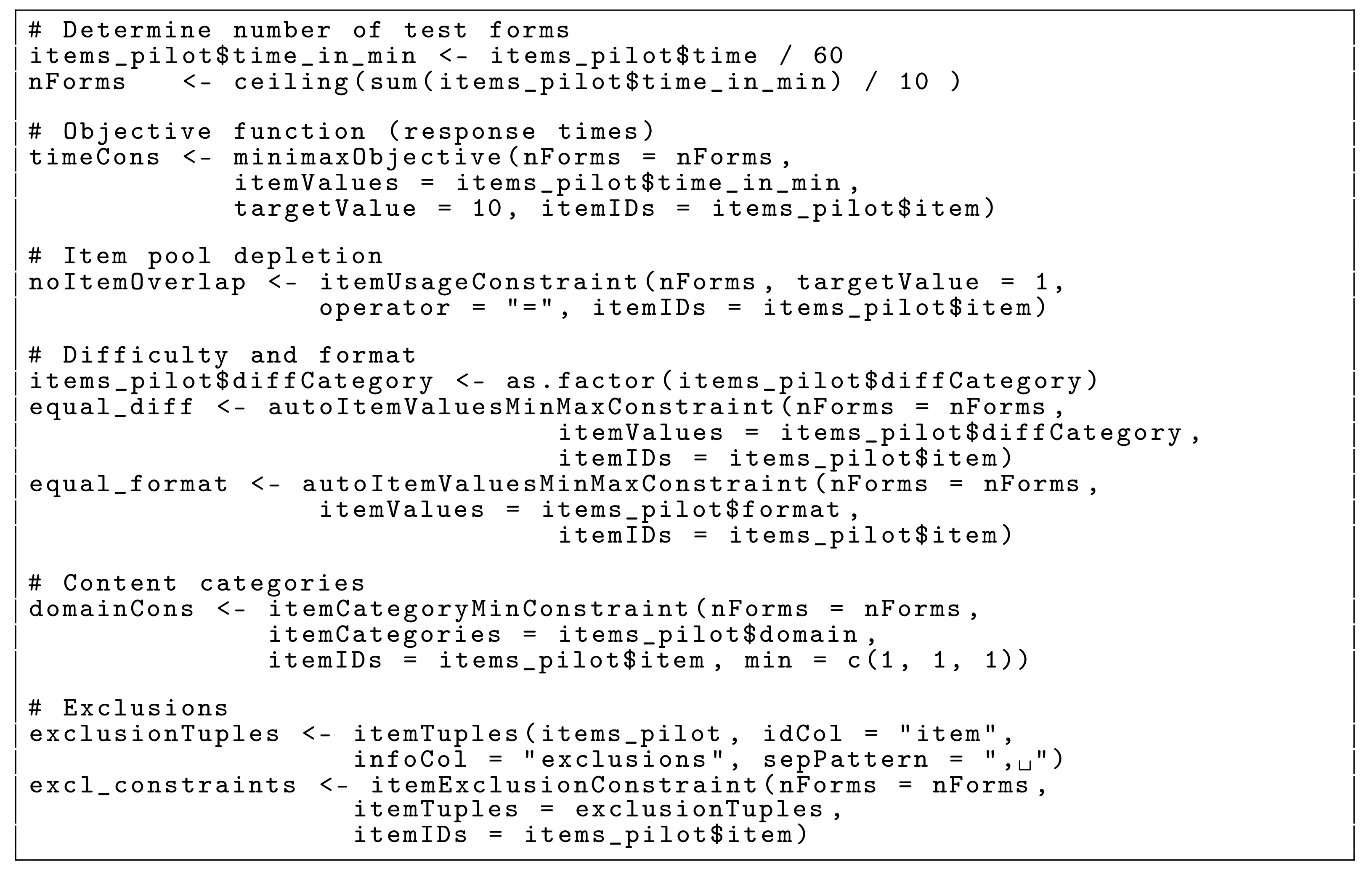
3.1. Pilot Study
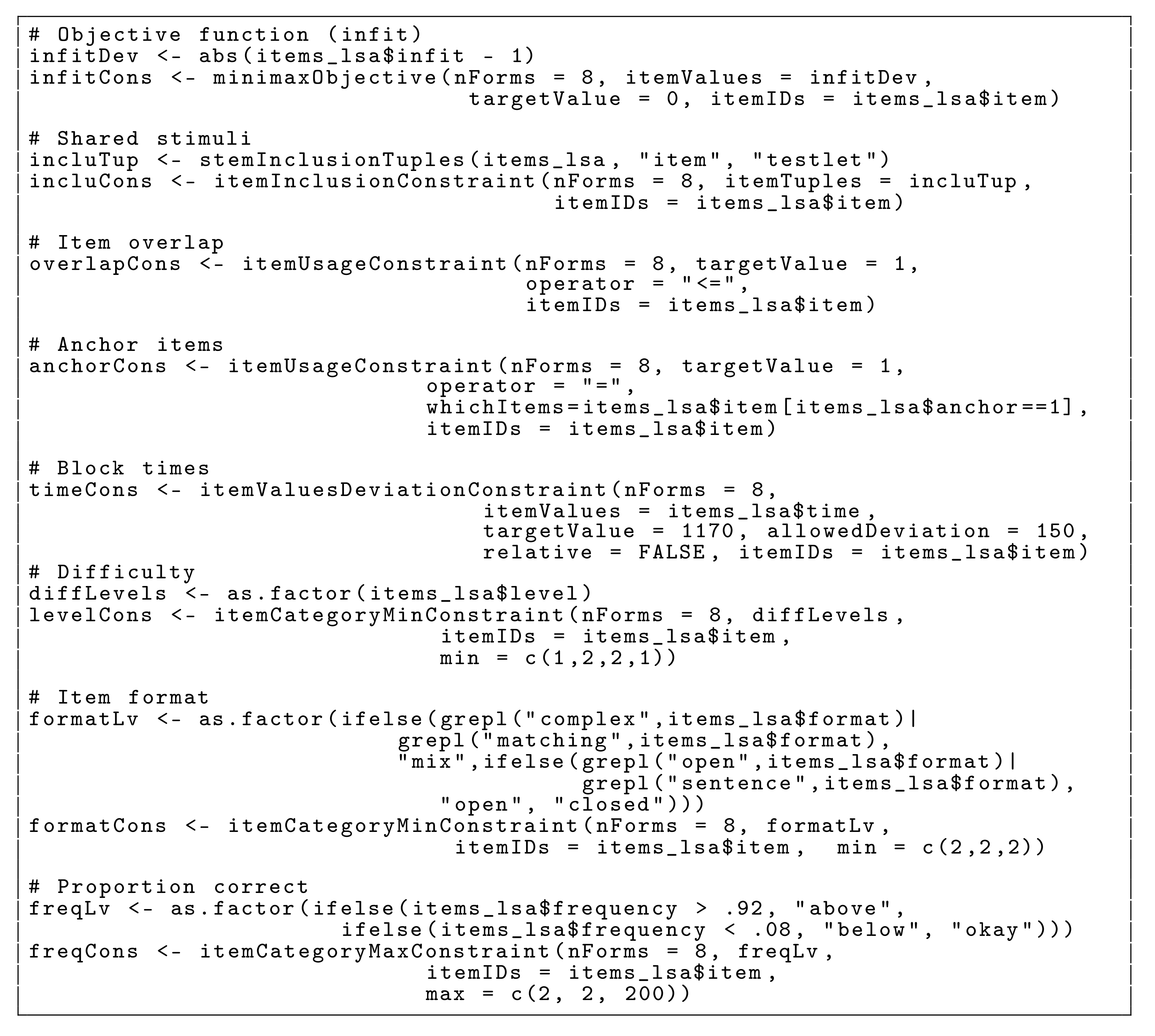
3.2. LSA Blocks for Multiple Matrix Booklet Designs
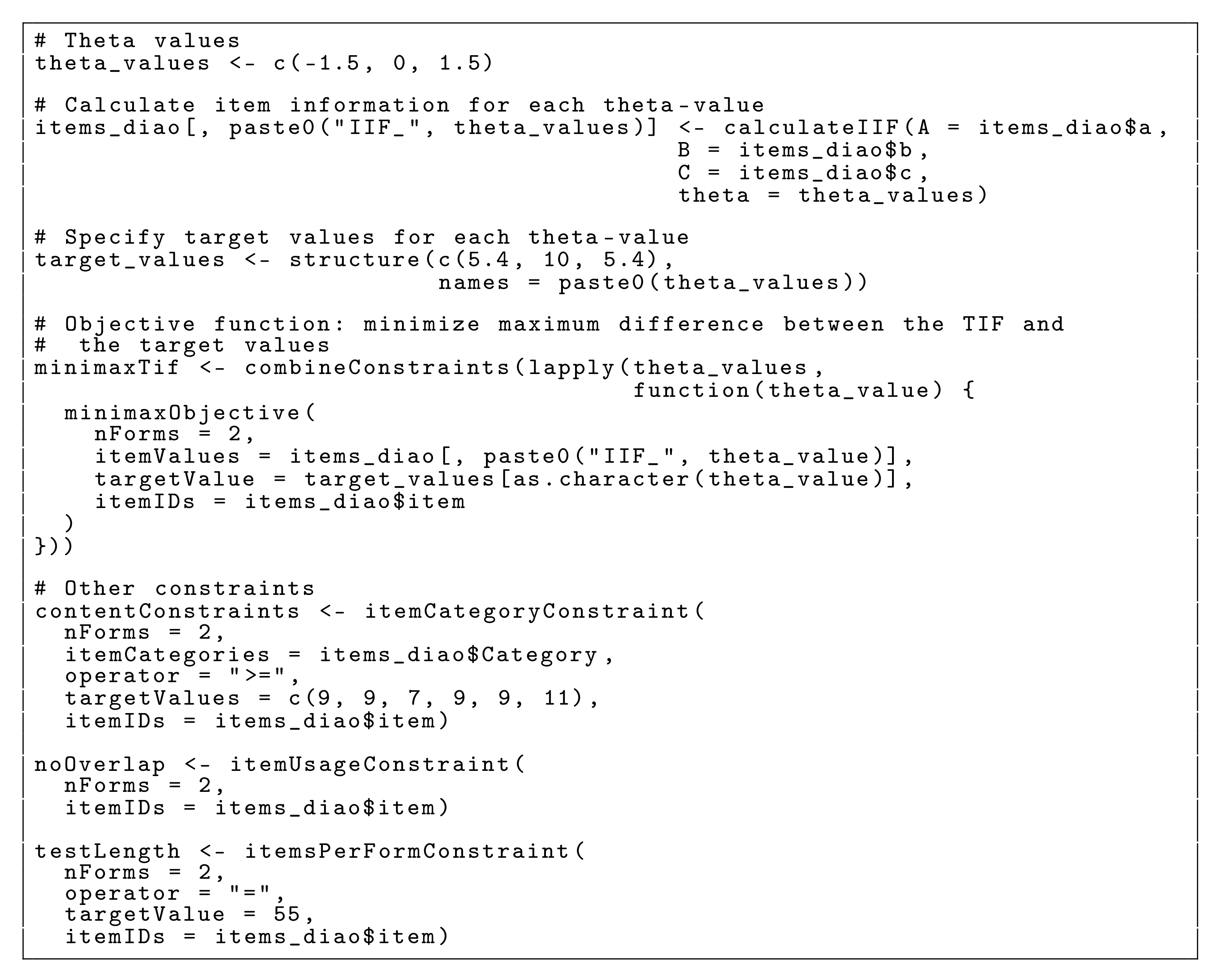
3.3. High-Stakes Assessment
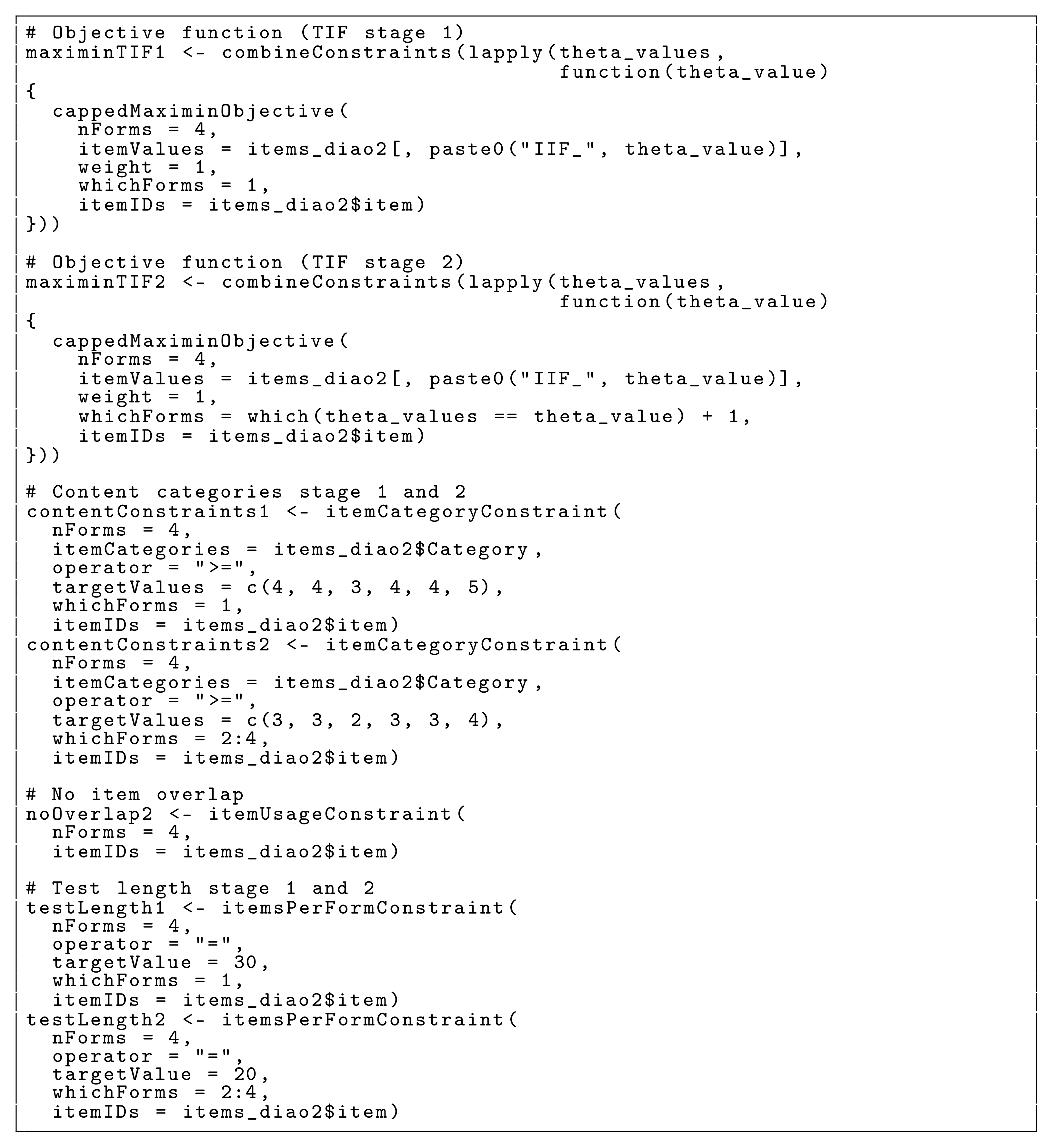
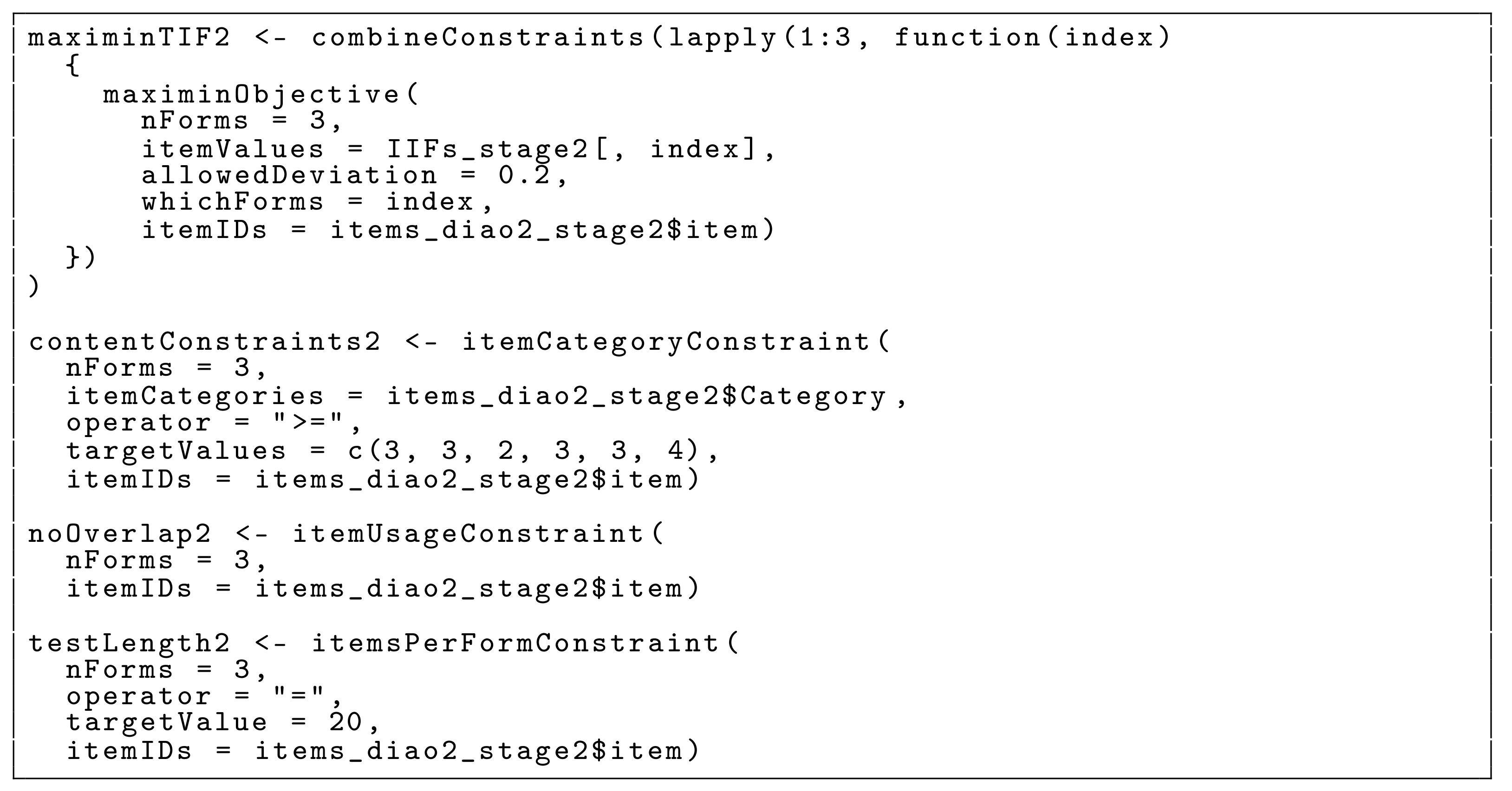
3.4. Multi-Stage Testing
3.4.1. Original Approach
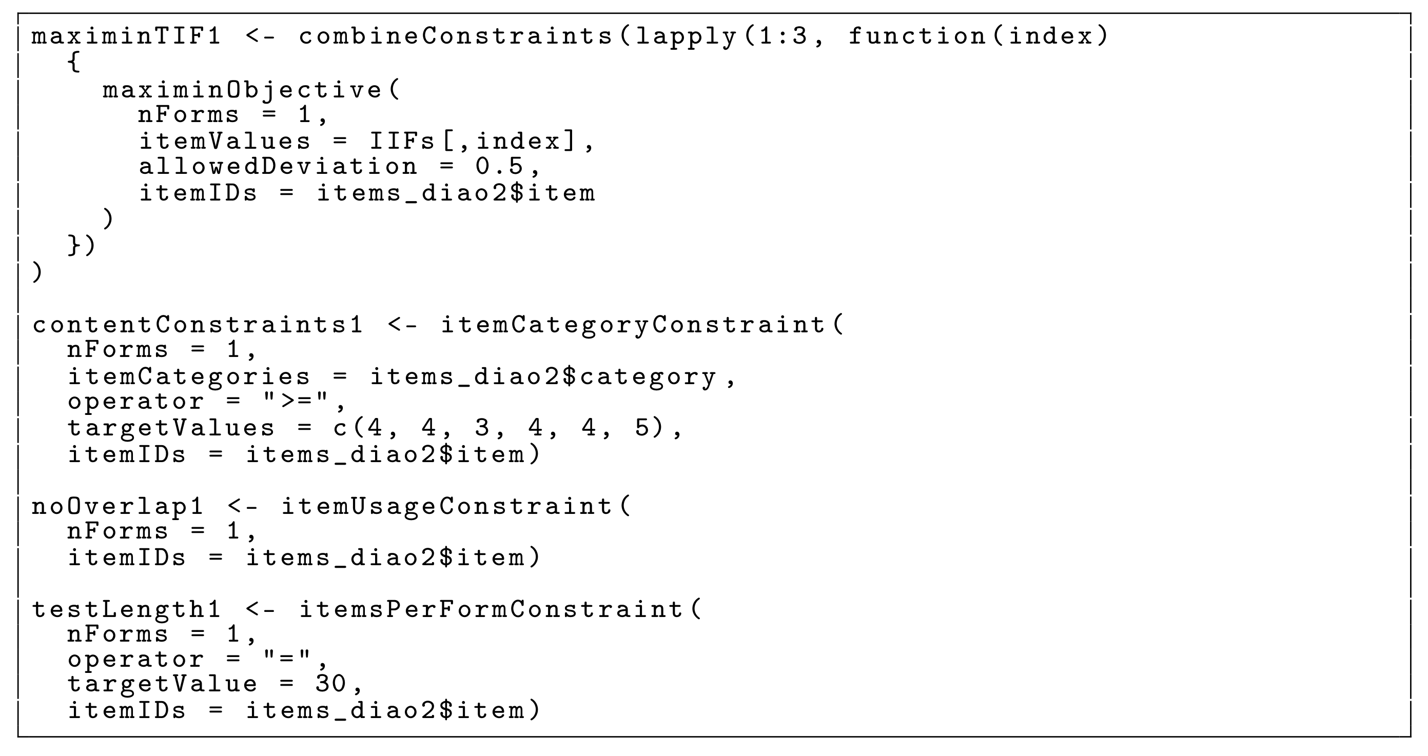
3.4.2. Combined Capped Approach
4. Discussion
4.1. Limitations
4.2. Alternatives
4.3. Conclusions
Supplementary Materials
Author Contributions
Funding
Institutional Review Board Statement
Informed Consent Statement
Data Availability Statement
Acknowledgments
Conflicts of Interest
Abbreviations
| ATA | Automated Test Assembly |
| MIP | Mixed-integer Programming |
| CAT | Computerized Adaptive Testing |
| MST | Multi-stage Testing |
| LSA | Large-scale Assessment |
| HST | High-stakes Assessment |
| IIF | Item Information Function |
| TIF | Test Information Function |
Appendix A
Appendix B

| Item | diffCategory | Format | Domain | Time | Exclusions |
|---|---|---|---|---|---|
| 1 | 2 | cmc | listening | 44.54 | |
| 2 | 4 | cmc | listening | 44.81 | |
| 3 | 4 | mc | writing | 32.36 | 76 |
| 4 | 2 | mc | listening | 48.03 | |
| 5 | 2 | mc | writing | 42.06 | 9 |
Appendix C
| Testlet | Item | Level | Format | Frequency | Infit | Time | Anchor |
|---|---|---|---|---|---|---|---|
| TRA5308 | TRA5308a | IV | multiple choice | 0.19 | 1.22 | 54.00 | 0 |
| TRA5308 | TRA5308b | IV | multiple choice | 0.24 | 1.01 | 66.00 | 0 |
| TRA5308 | TRA5308c | II | multiple choice | 0.42 | 1.22 | 89.00 | 0 |
| TRA5308 | TRA5308d | III | multiple choice | 0.41 | 1.21 | 92.00 | 0 |
| TRB6832 | TRB6832a | III | open answer | 0.51 | 1.21 | 85.00 | 0 |
| TRB6832 | TRB6832b | III | open answer | 0.20 | 1.08 | 61.00 | 0 |
| TRB6832 | TRB6832c | IV | open answer | 0.33 | 1.25 | 84.00 | 0 |
| TRB6832 | TRB6832d | II | open answer | 0.49 | 1.05 | 109.00 | 0 |
| TRC9792 | TRC9792a | I | cmc | 0.70 | 1.10 | 94.00 | 0 |
| TRC9792 | TRC9792b | I | cmc | 0.61 | 1.02 | 110.00 | 0 |
Appendix D
| Item | a | b | c | Category |
|---|---|---|---|---|
| 1 | 0.54 | −0.09 | 0.17 | 6 |
| 2 | 0.71 | −1.07 | 0.24 | 1 |
| 3 | 0.84 | −1.11 | 0.17 | 2 |
| 4 | 1.38 | −0.71 | 0.21 | 3 |
| 5 | 1.26 | −0.44 | 0.12 | 4 |
Appendix E
| Cat. 1 | Cat. 2 | Cat. 3 | Cat. 4 | Cat. 5 | Cat. 6 | |
|---|---|---|---|---|---|---|
| Item Pool | 23 | 26 | 22 | 29 | 29 | 36 |
| HST | 9 | 9 | 7 | 9 | 9 | 11 |
| MST: Stage 1 | 4 | 4 | 3 | 4 | 4 | 5 |
| MST: Stage 2 | 3 | 3 | 2 | 3 | 3 | 4 |
Appendix F


References
- Van der Linden, W.J. Linear Models for Optimal Test Assembly; Springer: New York, NY, USA, 2005. [Google Scholar]
- Luecht, R.M.; Sireci, S.G. A Review of Models for Computer-Based Testing; Research Report 2011-12; College Board: New York, NY, USA, 2011. [Google Scholar]
- Kuhn, J.T.; Kiefer, T. Optimal test assembly in practice. Z. Für Psychol. 2015, 221, 190–200. [Google Scholar] [CrossRef]
- OECD. PISA 2018 Technical Report; Technical Report; OECD Publishing: Paris, France, 2019. [Google Scholar]
- Yan, D.; Von Davier, A.A.; Lewis, C. Computerized Multistage Testing: Theory and Applications; CRC Press: Boca Raton, FL, USA, 2016. [Google Scholar]
- Van der Linden, W.J.; Glas, C.A. Computerized Adaptive Testing: Theory and Practice; Kluwer Academic Publishers: New York, NY, USA, 2000. [Google Scholar]
- R Core Team. R: A Language and Environment for Statistical Computing; R Foundation for Statistical Computing: Vienna, Austria, 2020. [Google Scholar]
- Konis, K.; Schwendinger, F. lpSolveAPI: R Interface to ‘lp_solve’ Version 5.5.2.0, R Package Version 5.5.2.0-17.7; 2020. Available online: https://CRAN.R-project.org/package=lpSolveAPI (accessed on 20 May 2021).
- Diao, Q.; van der Linden, W.J. Automated test assembly using lp_solve version 5.5 in R. Appl. Psychol. Meas. 2011, 35, 398–409. [Google Scholar] [CrossRef]
- Becker, B.; Debeer, D. eatATA: Create Constraints for Small Test Assembly Problems, R Package Version 0.11.2; 2021. Available online: https://CRAN.R-project.org/package=eatATA (accessed on 20 May 2021).
- Makhorin, A. GLPK (GNU Linear Programming Kit). 2018. Available online: https://www.gnu.org/software/glpk/ (accessed on 20 May 2021).
- Berkelaar, M.; Eikland, K.; Notebaert, P. lp_solve 5.5.2.5. 2016. Available online: http://lpsolve.sourceforge.net/5.5/ (accessed on 20 May 2021).
- Ladanyi, L.; Ralphs, T.; Menal, G.; Mahajan, A. coin-or/SYMPHONY: Version 5.6.17. 2019. Available online: https://projects.coin-or.org/SYMPHONY (accessed on 20 May 2020).
- Gurobi Optimization, LLC. Gurobi Optimizer Reference Manual; Gurobi Optimization, LLC: Houston, TX, USA, 2021. [Google Scholar]
- Theussl, S.; Hornik, K. Rglpk: R/GNU Linear Programming Kit Interface, R Package Version 0.6-4; 2019. Available online: https://CRAN.R-project.org/package=Rglpk (accessed on 20 May 2020).
- Berkelaar, M.; Csárdi, G. lpSolve: Interface to ’Lp_solve’ v. 5.5 to Solve Linear/Integer Programs; R Package Version 5.6.15; 2020; Available online: https://CRAN.R-project.org/package=lpSolve (accessed on 20 May 2021).
- Harter, R.; Hornik, K.; Theussl, S. Rsymphony: SYMPHONY in R, R Package Version 0.1-29; 2020. Available online: https://CRAN.R-project.org/package=Rsymphony (accessed on 20 May 2021).
- Gurobi Optimization, LLC. Gurobi: Gurobi Optimizer 9.1 interface, R package version 9.1-1; Gurobi Optimization, LLC: Houston, TX, USA, 2021. [Google Scholar]
- Donoghue, J.R. Comparison of Integer Programming (IP) Solvers for Automated Test Assembly (ATA); Research Report 15-05; Educational Testing Service: Princeton, NJ, USA, 2015. [Google Scholar]
- Luo, X. Automated Test Assembly with Mixed-Integer Programming: The Effects of Modeling Approaches and Solvers. J. Educ. Meas. 2020, 57, 547–565. [Google Scholar] [CrossRef]
- Rasch, G. Studies in Mathematical Psychology: I. Probabilistic Models for Some Intelligence and Attainment Tests; Nielsen & Lydiche: Copenhagen, Denmark, 1960. [Google Scholar]
- Spaccapanico Proietti, G.; Matteucci, M.; Mignani, S. Automated Test Assembly for Large-Scale Standardized Assessments: Practical Issues and Possible Solutions. Psych 2020, 2, 315–337. [Google Scholar] [CrossRef]
- Gonzalez, E.; Rutkowski, L. Principles of multiple matrix booklet design and parameter recovery in large-scale assessments. In IERI Monograph Series: Issues and Methodologies in Large-Scalse Assessments: Volume 3; von Davier, M., Hastedt, D., Eds.; IEA-ETS Research Institute: Hamburg, Germany, 2010; pp. 125–156. [Google Scholar]
- Frey, A.; Hartig, J.; Rupp, A.A. An NCME instructional module on booklet designs in large-scale assessments of student achievement: Theory and practice. Educ. Meas. Issues Pract. 2009, 28, 39–53. [Google Scholar] [CrossRef]
- Pokropek, A. Missing by design: Planned missing-data designs in social science. Res. Methods 2011, 20, 81–105. [Google Scholar]
- Kolen, M.J.; Brennan, R.L. Test Equating, Scaling, and Linking: Methods and Practices; Springer Science & Business Media: New York, NY, USA, 2014. [Google Scholar]
- OECD. PISA 2012 Technical Report; Technical Report; OECD Publishing: Paris, France, 2014. [Google Scholar]
- Choi, S.W.; Lim, S. TestDesign: Optimal Test Design Approach to Fixed and Adaptive Test Construction, R Package Version 1.2.2; 2021. Available online: https://CRAN.R-project.org/package=TestDesign (accessed on 20 May 2021).
- Jiang, B. RSCAT: Shadow-Test Approach to Computerized Adaptive Testing, R Package Version 1.1.0; 2021. Available online: https://CRAN.R-project.org/package=RSCAT (accessed on 20 May 2021).
- Luo, X. Rata: Automated Test Assembly; R Package Version 0.0.2; 2019. Available online: https://CRAN.R-project.org/package=Rata (accessed on 20 May 2021).
- Luo, X. xxIRT: Item Response Theory and Computer-Based Testing in R, R Package Version 2.1.2; 2019. Available online: https://CRAN.R-project.org/package=xxIRT (accessed on 20 May 2021).
- Chang, T.Y.; Shiu, Y.F. Simultaneously construct IRT-based parallel tests based on an adapted CLONALG algorithm. Appl. Intell. 2012, 36, 979–994. [Google Scholar] [CrossRef]
- Sun, K.T.; Chen, Y.J.; Tsai, S.Y.; Cheng, C.F. Creating IRT-based parallel test forms using the genetic algorithm method. Appl. Meas. Educ. 2008, 21, 141–161. [Google Scholar] [CrossRef]
- Verschoor, A.J. Genetic Algorithms for Automated Test Assembly. Ph.D. Thesis, Twente University, Enschede, The Netherlands, 2007. [Google Scholar]
- Veldkamp, B.P. Multiple objective test assembly problems. J. Educ. Meas. 1999, 36, 253–266. [Google Scholar] [CrossRef]
- Van der Linden, W.J.; Li, J. Comment on three-element item selection procedures for multiple forms assembly: An item matching approach. Appl. Psychol. Meas. 2016, 40, 641–649. [Google Scholar] [CrossRef] [PubMed]


| Item | Format | Time | Difficulty | IIF_0 |
|---|---|---|---|---|
| 1 | mc | 27.79 | −1.88 | 0.11 |
| 2 | mc | 15.45 | 0.84 | 0.45 |
| 3 | mc | 31.02 | 1.12 | 0.33 |
| 4 | mc | 29.87 | 0.73 | 0.50 |
| 5 | mc | 23.13 | −0.49 | 0.61 |
Publisher’s Note: MDPI stays neutral with regard to jurisdictional claims in published maps and institutional affiliations. |
© 2021 by the authors. Licensee MDPI, Basel, Switzerland. This article is an open access article distributed under the terms and conditions of the Creative Commons Attribution (CC BY) license (https://creativecommons.org/licenses/by/4.0/).
Share and Cite
Becker, B.; Debeer, D.; Sachse, K.A.; Weirich, S. Automated Test Assembly in R: The eatATA Package. Psych 2021, 3, 96-112. https://doi.org/10.3390/psych3020010
Becker B, Debeer D, Sachse KA, Weirich S. Automated Test Assembly in R: The eatATA Package. Psych. 2021; 3(2):96-112. https://doi.org/10.3390/psych3020010
Chicago/Turabian StyleBecker, Benjamin, Dries Debeer, Karoline A. Sachse, and Sebastian Weirich. 2021. "Automated Test Assembly in R: The eatATA Package" Psych 3, no. 2: 96-112. https://doi.org/10.3390/psych3020010
APA StyleBecker, B., Debeer, D., Sachse, K. A., & Weirich, S. (2021). Automated Test Assembly in R: The eatATA Package. Psych, 3(2), 96-112. https://doi.org/10.3390/psych3020010