Appendix A
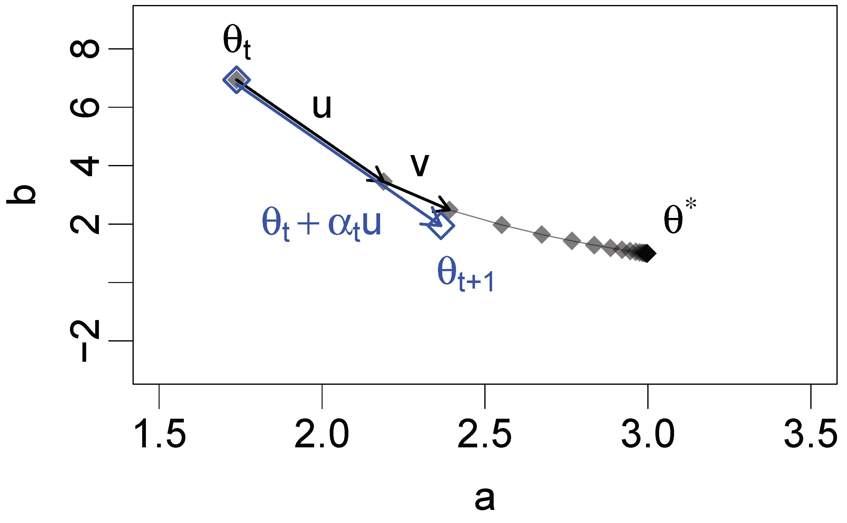
Algorithm A1 shows pseudocode for the QN method, based on a simplified representation of the QN implementation within the
turboEM:::accelerate and
turboEM::: bodyQuasiNewton methods [
28]. The algorithm starts with initial parameters
. First, the
q columns of matrix
U are created from a sequence of EM updates (
F; Algorithm A1, lines 1–11). Then, matrix
V is created based on
U and a further EM update (Algorithm A1, lines 12–16). Finally, QN updates are performed until convergence (Algorithm A1, lines 17–27). Algorithm A1 only shows a skeleton of the QN method. The implementation of the QN update in
turboEM:::bodyQuasiNewton is a little more complex. For instance, parameter constraints can be supplied by the user to keep the parameter updates in
turboEM:::bodyQuasiNewton within certain bounds [
28]. Perhaps more importantly, there is an additional check that the negative log-likelihood is decreased (i.e., the log-likelihood is increased) by the QN update
compared to the last EM update
. If
, the value of
is set to
instead [
28]. This modification is used to ensure global convergence.
| Algorithm A1: Pseudocode for QN |
 |
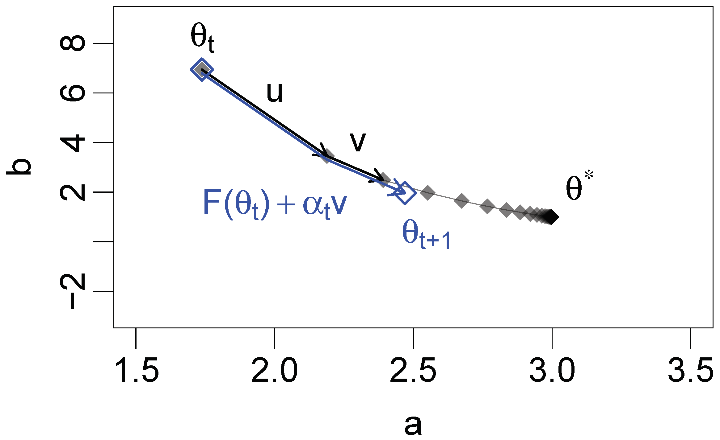
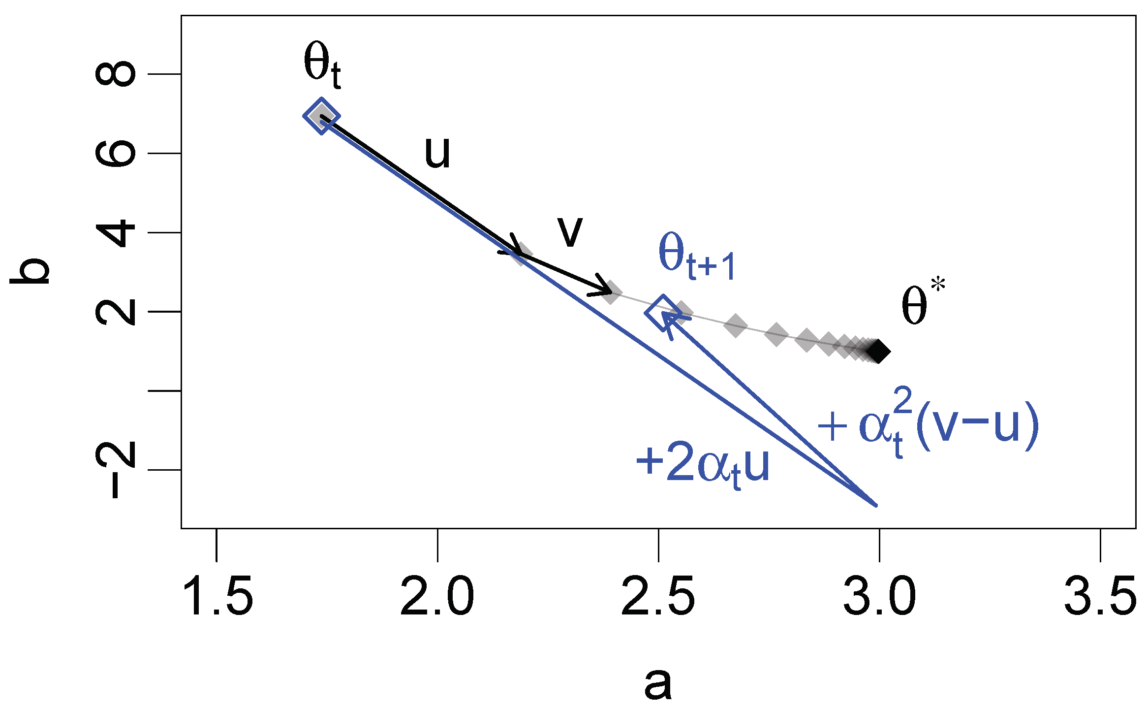
Algorithm A2 shows pseudocode for the first-order SQUAREM method, based on [
13]. It is consistent with the SQUAREM implementation within the
turboEM:::accelerate and
turboEM:::bodySquarem1 methods [
28]. The algorithm operates on an input of initial parameter estimates
. Based on these parameters, the algorithm is run until convergence. First, two successive EM updates are performed (Algorithm A2, lines 2–3) to calculate
u and
v (Algorithm A2, lines 4–5). Based on
u and
v, the steplength
is computed (Algorithm A2, line 6). For global convergence, the steplength is modified if necessary (Algorithm A2, line 7). Then, the SQUAREM update is computed (Algorithm A2, line 8). Finally, an EM update of the SQUAREM update provides a new parameter estimate for the next iteration [
13,
28]. The algorithm can be run in three versions, “1”, “2”, or “3”, depending on which steplength is to be used. By default, the
turboEM:::bodySquarem1 method uses steplength S3, as recommended by [
13]. The implementation of Algorithm A2 in the
turboEM:::bodySquarem1 method includes additional checks on the SQUAREM update [
28]. For instance, if the user has specified constraints on the parameter space, the update must fall within the constraints. If the SQUAREM update does not increase the log-likelihood, the last EM update is used instead. Finally, upper and lower bounds are set on the steplength and modified dynamically to increase stability and convergence [
28]. Pseudo-code for higher-order SQUAREM is not shown here.
| Algorithm A2: Pseudocode for SQUAREM () |
 |
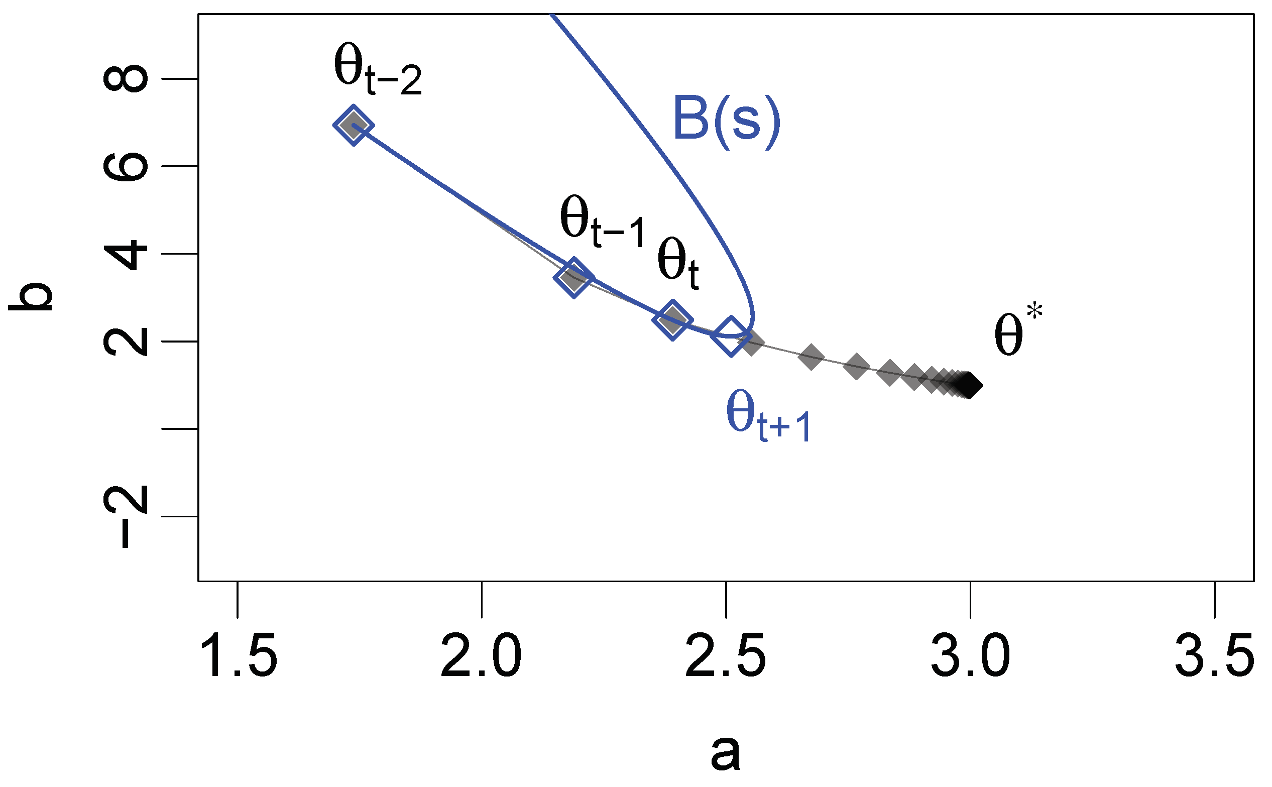
Algorithm A3 shows pseudocode for the PEM acceleration method, consistent with the implementation of PEM in the
turboEM:::bodyParaEM method [
14,
28]. First, an initial PEM update is computed for an initial value of the search parameter
s (Algorithm A3, lines 2–4). If the log-likelihood is not increased by this PEM update, then the PEM update is disregarded and regular EM updates are performed instead (Algorithm A3, lines 5–9). If the log-likelihood does increase, further PEM updates are performed for increasing values of
s, until the log-likelihood no longer increases (Algorithm A3, lines 11–18). The last PEM update for which the log-likelihood increased is retained, and two regular EM updates are performed on this PEM update to create the next member of the parameter estimation sequence (Algorithm A3, lines 19–22). According to [
14], these two EM updates performed on the final PEM update stabilize the algorithm. Finally, the procedure is repeated until convergence.
| Algorithm A3: Pseudocode for PEM |
 |
Appendix E
In this appendix, we wanted to give a brief impression of how far our results for IRT—in particular, 1PL and 2PL—models are likely to generalize to other model classes. To this end, we briefly examined the accelerators’ performance in the context of the Maximum Likelihood (ML) estimation for Gaussian mixture models (GMM). A Gaussian mixture model describes an observable random variable
X with a multimodal distribution generated by the sum of
K subpopulations of
X. Each subpopulation
is produced by an independent random variable
, which follows a multivariate (
d-dimensional) normal distribution with expected value
and variance
. A latent, multinomial random variable
Z determines which subpopulation
a given value of
X comes from. In other words,
X can be written as [
9]
Here,
is an indicator function, which equals 1 if
and 0 otherwise. For a given subpopulation
k,
X therefore follows a multivariate normal distribution, i.e., the conditional probability density function of
X given
is
for
with
and
[
9]. Because
Z is a multinomial variable, the probability distribution of
Z is given by
, with
. The marginal log-likelihood for the GMM is given by [
9]:
Assuming that the GMM is a widely known model and its estimation with the EM algorithm is a standard application of the EM algorithm, we are not going to go into more detail here with the model description or the EM algorithm for this model, but instead refer the interested reader to [
9]. In the following, we are going to describe a brief simulation aimed at garnering an impression of how the accelerators behave in a different model class. To reduce complexity in this brief additional simulation comprising four different settings, only two subpopulations are considered (
), where
is the probability of being in the first subpopulation, and
. To reduce complexity further, the first three settings deal only with one dimension (
), whereas the fourth setting studies the effect of increasing the number of dimensions. During the maximization step, the optimization of
is independent of all other parameters (for
), and the optimizations of the parameters of the subpopulations are independent of each other, although of course, the optimization depends on the membership probabilities calculated during the expectation step, which depend on all parameters. Still, to study the properties of the EM algorithm, it is illustrative to vary only the parameters of one subpopulation. The first subpopulation shall be distributed as
and the second subpopulation as
. Then, three simple cases are studied that are illustrative in their simplicity, but still also relevant in the sense that many one-dimensional datasets can be transformed in such a way that they fall into one of these categories. Furthermore, to study the effect of increasing the dimensions of
, a fourth setting is examined:
- Setting 1.
Let be known, and variances be equal . In this case, acceleration of the EM algorithm for the estimation of proportions is examined. Because can be optimized independently of all other parameters, all other parameters are kept constant.
- Setting 2.
Let be known, and variances be equal . In this case, acceleration of the EM algorithm for the estimation of location and equal variance in two subpopulations is investigated. Because is independent of the parameters of the second subpopulation, its estimation is no longer of interest, and it is kept constant.
- Setting 3.
Let be known . In this case, acceleration of the EM algorithm for the estimation of location and variance of one subpopulation is analyzed. Because , and are independent of the parameters of the second subpopulation, their estimation is no longer of interest.
- Setting 4.
Let be known, and and be unknown . By increasing the dimension of X (), the dimension of is increased to . This case addresses the question of how this increase in dimensions affects the acceleration of the EM algorithm.
To ensure comparability between the four settings in this brief additional simulation, a single Gaussian mixture dataset is simulated. The simulated dataset is shown in
Figure A3. The total number of observations is
N = 100,000 (as in the main simulations of this work, this is to examine a large-assessment setting; as we have also seen in the main simulations, results may be different in smaller samples). For
(Settings 1–3), the dataset is characterized by the real parameter values of
,
,
,
, and
. For
(Setting 4), the same data are used for the first dimension, but additional dimensions are simulated with the real parameter values
and
(not shown).
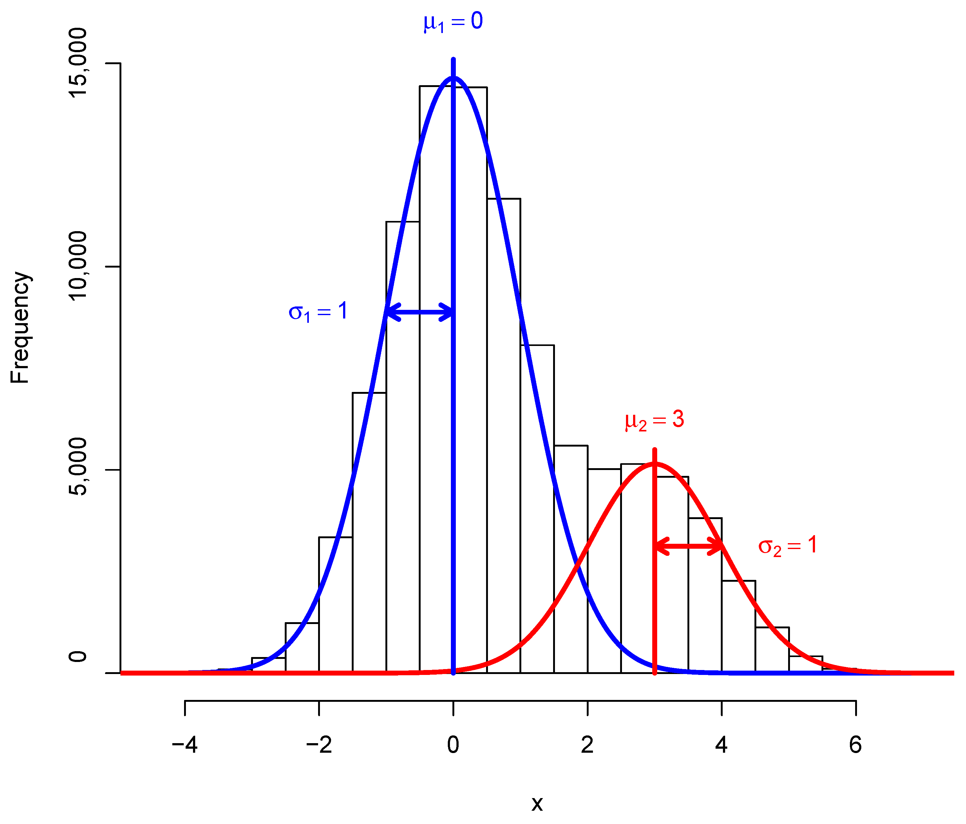
Figure A3.
Simulated Gaussian mixture model (GMM) dataset in one dimension () with two subpopulations (). Blue: the first subpopulation. Red: the second subpopulation. The dataset is simulated in R with the rnorm function and parameter values , , , , and . The total number of observations in the dataset is .
In the following, we are going to present the results obtained from this brief simulation, in which we compared the acceleration methods described in the main text in the four settings outlined above. The implementation of the simulation in R is similar to what we have described in the main text for the IRT simulation, and thus will not be reiterated here. For this brief simulation, which was mostly intended as an illustration of the accelerators’ behavior in model classes other than (logistic) IRT models, we only ran 16 trials in each setting, which were characterized by 16 different starting values for (ranging from 0.05 to 0.95 in equidistanced steps for the first setting), as well as by 16 different pairs of starting values for and or (ranging from 0 to 6 for , and 0.1 to 3 for ) for the second and third setting, respectively. The starting values and in setting 4 were the same as in setting 3; the starting values for are set to zero.
For the most simple setting, setting 1, in which we only estimate one parameter, only the first-order variants of SQUAREM and QN are studied. For PEM, only three initial EM updates that do not count towards the total number of iterations were performed. In line with the main simulations of this work, default tuning parameters were used (otherwise). As convergence criterion,
was used because it does not require additional evaluations of the log-likelihood. The results, averaged for the 16 runs, are shown in
Table A9. All three methods studied (QN (
), SQUAREM (
), and PEM) converge to the fixed point in all 16 runs (
Table A9). The total number of iterations required to reach the fixed point is reduced three- to four-fold on average in all three methods studied compared to standard EM, from 11 to 3 (QN) or 4 (SQUAREM and PEM;
Table A9). However, since the acceleration methods do require at least two evaluations of
F per iteration, the total number of
F evaluations is only reduced by less than half in QN and SQUAREM (from 11 to 6 or 7) and not greatly reduced with PEM (from 11 to 10), which has to perform three additional EM updates to obtain initial points for the Bezier parabola before it can start. As expected, the number of log-likelihood evaluations is larger for the accelerated methods than for EM, increasing the acceleration cost. However, even so, the CPU time spent on QN and SQUAREM is greatly reduced (
Table A9). For PEM, which has the highest number of log-likelihood evaluations due to exploration of the parameter space, the CPU time actually increases compared to EM. However, perhaps in this example, there is not much scope for PEM to show its full power because even the standard EM algorithm only requires 11 steps for completion.
Table A9.
EM acceleration results for GMM setting 1 based on runs performed in R with the package turboEM, with the sixteen different starting values, and with as the convergence criterion. The numbers shown represent a rounded average over the sixteen runs. MLE: Maximum likelihood estimate (fixed point); : Average number of iterations from the starting value to the fixed point; Fevals: Average number of F evaluations; Levals: Average number of log-likelihood evaluations; Conv.: Fraction of converging runs; CPU: Average CPU time in milliseconds; Rel. Time: Computing time relative to standard EM.
| | Method | MLE () | | Fevals | Levals | Conv. | CPU (ms) | Rel. Time |
|---|
| | EM | (0.7496) | 11 | 11 | 1 | 1.00 | 11.62 | 1.00 |
| | QN () | (0.7496) | 3 | 6 | 6 | 1.00 | 8.69 | 0.75 |
| | SQUAREM () | (0.7496) | 4 | 7 | 5 | 1.00 | 10.38 | 0.89 |
| | PEM | (0.7496) | 4 | 10 | 14 | 1.00 | 14.81 | 1.27 |
The average EM acceleration results across the 16 different starting values for the second setting are shown in
Table A10. Because
is two-dimensional, higher-order QN (
) and SQUAREM (
) can now be analyzed in addition to QN (
), SQUAREM (
) and PEM. All algorithms converge in all trials. Like in Case 1, there is an almost four-fold reduction in the total number of iterations needed to reach the fixed point (from 22 on average to 6 on average;
Table A10). Again, all acceleration methods behave fairly similarly; there is also no great difference between QN (
) and QN (
). SQUAREM (
) and PEM require a large number of
F evaluations (20 and 15, respectively), which is close to standard EM (22;
Table A10). However, in terms of CPU time, SQUAREM (
) still performs second best, with SQUAREM (
) performing the best (
Table A10).
Setting 3 loosens the assumption of the variance
being equal in the two subpopulations, leading us to estimate
and
in the second subpopulation, while we assume the remaining parameters to be known. In this setting, EM acceleration is performed with the same techniques as for the second setting. All runs converge, and the number of iterations required to reach the fixed point is reduced five-fold or more by the accelerators (
Table A11). Of the five acceleration methods studied (QN (
), QN (
), SQUAREM (
), SQUAREM (
), and PEM), the second-order QN as well as the two SQUAREM methods perform best in terms of CPU time (
Table A11).
Table A10.
EM acceleration results for GMM setting 2 based on runs performed in R with the package turboEM, with the sixteen different starting values, and with as the convergence criterion. The numbers shown represent a rounded average over the sixteen runs. MLEs: Maximum likelihood estimates (fixed point); : Average number of iterations from the starting value to the fixed point; Fevals: Average number of F evaluations; Levals: Average number of log-likelihood evaluations; Conv.: Fraction of converging runs; CPU: Average CPU time in milliseconds; Rel. Time: Computing time relative to standard EM.
| | Method | MLEs () | | Fevals | Levals | Conv. | CPU (ms) | Rel. Time |
|---|
| | EM | (2.9963, 1.0009) | 22 | 22 | 1 | 1.00 | 36.81 | 1.00 |
| | QN () | (2.9963, 1.0009) | 6 | 9 | 12 | 1.00 | 31.69 | 0.86 |
| | QN () | (2.9963, 1.0009) | 6 | 10 | 12 | 1.00 | 34.50 | 0.94 |
| | SQUAREM () | (2.9963, 1.0009) | 6 | 10 | 6 | 1.00 | 29.00 | 0.79 |
| | SQUAREM () | (2.9963, 1.0009) | 4 | 20 | 5 | 1.00 | 35.25 | 0.96 |
| | PEM | (2.9963, 1.0009) | 6 | 15 | 29 | 1.00 | 36.44 | 0.99 |
Table A11.
EM acceleration results for GMM setting 3 based on runs performed in R with the package turboEM, with the sixteen different starting values, and with as the convergence criterion. The numbers shown represent a rounded average over the sixteen runs. MLEs: Maximum likelihood estimates (fixed point); : Average number of iterations from the starting value to the fixed point; Fevals: Average number of F evaluations; Levals: Average number of log-likelihood evaluations; Conv.: Fraction of converging runs; CPU: Average CPU time in milliseconds; Rel. Time: Computing time relative to standard EM.
| | Method | MLEs () | | Fevals | Levals | Conv. | CPU (ms) | Rel. Time |
|---|
| | EM | (2.9979, 0.9953) | 40 | 40 | 1 | 1.00 | 53.88 | 1.00 |
| | QN () | (2.9979, 0.9953) | 8 | 12 | 17 | 1.00 | 36.44 | 0.67 |
| | QN () | (2.9979, 0.9953) | 6 | 10 | 13 | 1.00 | 27.75 | 0.52 |
| | SQUAREM () | (2.9979, 0.9953) | 7 | 12 | 8 | 1.00 | 26.25 | 0.49 |
| | SQUAREM () | (2.9979, 0.9953) | 4 | 22 | 5 | 1.00 | 25.94 | 0.48 |
| | PEM | (2.9979, 0.9953) | 8 | 19 | 42 | 1.00 | 43.50 | 0.81 |
Finally, in setting 4, we increased the number of dimensions of
X from
to
. Like in setting 3, the parameters of the first subpopulation are considered known. In higher dimensions, these parameters are
,
, and
. The parameters of the second subpopulation are to be estimated:
, and
. The unknown parameter vector is therefore given by
—it has
dimensions. In this setting, it takes fewer iterations to reach the fixed point (even with just standard EM), as few as half of those required in setting 3. The reason for faster convergence may be that more data are available to estimate
. As
is 11-dimensional, even higher orders of QN (
q > 2) and SQUAREM (
k > 2) methods can be studied (
Table A12). As in the other three cases, QN, SQUAREM, and PEM accelerate the EM algorithm four- to five-fold in terms of number of iterations (
Table A12). However, it is worth noting that SQUAREM (
) and SQUAREM (
) actually use a higher number of
F evaluations than the standard EM algorithm, and so do not improve on it for those scores (
Table A12). PEM hardly accelerates the EM algorithm, while the higher-order SQUAREM methods actually decelerate it. Overall, acceleration in terms of CPU time is not very strong in terms of magnitude, with a maximum reduction of about 20% for QN (
) (
Table A12).
Overall, the GMM analysis shows that all three acceleration techniques—QN, SQUAREM, and PEM-work well for Gaussian mixture models (
Table A9,
Table A10,
Table A11,
Table A12). The four- to five-fold decrease in the number of iterations is consistent with what has been observed in previous studies for other models [
10,
12,
13,
14]. In the context of Gaussian mixture models, PEM is consistently more expensive in terms of the number of evaluations of
F and the log-likelihood, and also in terms of CPU time. However, in all four cases, even the high-dimensional one, the fixed point is reached relatively quickly. Perhaps differences in the three acceleration methods will become more apparent in contexts where the standard EM algorithm requires a much higher number of iterations to reach the fixed point. This leads us to the recommendation we have formulated in our discussion of studying the accelerators discussed in this work in the context of other, more complex model classes.
Table A12.
EM acceleration results for GMM setting 4 () based on runs performed in R with the package turboEM, with the sixteen different starting values, and with as the convergence criterion. The numbers shown represent a rounded average over the sixteen runs. For comparison with setting 3, only the maximum likelihood estimates for and are shown. MLEs: Maximum likelihood estimates (fixed point); : Average number of iterations from the starting value to the fixed point; Fevals: Average number of F evaluations; Levals: Average number of log-likelihood evaluations; Conv.: Fraction of converging runs; CPU: Average CPU time in milliseconds; Rel. Time: Computing time relative to standard EM.
| | Method | MLEs () | | Fevals | Levals | Conv. | CPU (ms) | Rel. Time |
|---|
| | EM | (2.9971, 0.998) | 19 | 19 | 1 | 1.00 | 570.69 | 1.00 |
| | QN () | (2.9971, 0.998) | 6 | 9 | 12 | 1.00 | 497.69 | 0.87 |
| | QN () | (2.9971, 0.998) | 5 | 9 | 10 | 1.00 | 490.75 | 0.86 |
| | QN () | (2.9971, 0.998) | 4 | 10 | 9 | 1.00 | 488.19 | 0.86 |
| | QN () | (2.9971, 0.998) | 4 | 10 | 7 | 1.00 | 459.75 | 0.81 |
| | SQUAREM () | (2.9971, 0.998) | 5 | 10 | 6 | 1.00 | 502.94 | 0.88 |
| | SQUAREM () | (2.9971, 0.998) | 3 | 17 | 4 | 1.00 | 543.50 | 0.95 |
| | SQUAREM () | (2.9971, 0.998) | 3 | 21 | 4 | 1.00 | 663.12 | 1.16 |
| | SQUAREM () | (2.9971, 0.998) | 2 | 22 | 3 | 1.00 | 675.44 | 1.18 |
| | PEM | (2.9971, 0.998) | 6 | 15 | 25 | 1.00 | 623.56 | 1.09 |


