Surfactant Temperature-Dependent Critical Micelle Concentration Prediction with Uncertainty-Aware Graph Neural Network

Abstract

The critical micelle concentration (CMC) is a fundamental physicochemical property of surfactants with significant implications across multiple industries. This paper presents an uncertainty-aware graph neural network (GNN) that integrates molecular structure and temperature to simultaneously predict CMC values and prediction uncertainties. Trained on a curated dataset of 2133 CMC values with temperature annotations, our GNN achieves comparatively similar performance on two external test sets from similar works. The model provides adequately calibrated uncertainty estimates that reliably quantify prediction confidence. This dual-output approach enables reliable CMC prediction with quantifiable confidence intervals, addressing a practical need for safety-critical applications where underestimation of uncertainty could have serious consequences.

1. Introduction

The critical micelle concentration (CMC) is one of the most important physicochemical properties of surfactants, with significant implications in the cosmetic, pharmaceutical, household, mining and gas and oil industries. The CMC is directly or indirectly related to surfactant’s surface activity, effective concentration, toxicity, biological activity, and other key characteristics. Due to the considerable structural diversity of surfactants, no comprehensive theoretical methods currently exist to predict CMC as a function of molecular structure.

Molecular dynamics (MD) and quantum-chemical-based quantitative structure–property relationship (QSPR) models have been previously employed for CMC prediction. Turchi et al. [1] presented a method, which employs first principles-based interfacial tension calculations rooted in quantum chemical COSMO-RS theory, for the prediction of the critical micelle concentration of a set of nonionic, cationic, anionic, and zwitterionic surfactants in aqueous solutions. Cárdenas et al. [2] determined interfacial tension and CMC of sugar-based nonionic surfactant n-dodecyl glucoside from atomistic molecular simulations. Approximated value of the CMC was obtained by geometrical analysis of the behavior of the interface.

Additionally, group-contribution methods and probabilistic approaches, including Markov chain modeling, have been applied for surfactant CMC prediction. Mattei et al. [3] developed an extended group-contribution model for predicting CMC values of nonionic surfactants in aqueous solutions at 25 °C. Smith et al. [4] employed a Markov chain model to predict CMC and surface composition in binary surfactant systems.

Conventional QSPR methods—relying on quantum chemical calculations, molecular dynamics simulations or other non-machine learning techniques—often entail high computational costs and remain limited in their ability to incorporate the influence of structural features. In contrast, cheminformatics has emerged as a robust paradigm for molecular design and property prediction, leveraging data-driven models to analyze chemical data of varying scales and complexity.

Machine learning (ML) has become an established tool in cheminformatics, demonstrating success in solving various problems [5,6,7,8], including CMC prediction. Early attempts at utilizing ML models for CMC prediction mostly are multiple linear regression (MLR) models used with different types of descriptors—topological [9,10], quantum-chemical [11,12] or their combination [13]—for CMC prediction of single-type surfactants (mostly nonionic or anionic). Subsequent research expanded descriptor diversity to include fragment-based and structural features [14,15]. A notable exception among them is the partial least squares (PLS) regression model by Anoune et al. [16], which was trained on a combination of different types of descriptors—ranging from compound molecular weight to various electrical (e.g., dipole moment) and topology-dependent properties—to predict CMC of multiple surfactant types. The methodological advancement continued with the adoption of artificial neural networks (ANN) [17,18,19,20], support vector regression (SVR) [15,18,20] and tree-based [20] methods, each demonstrating enhanced predictive capability for structurally diverse surfactants.

The latest advances in the field have focused on graph neural networks (GNNs) [21,22,23], which directly process molecular graph representations to capture complex structural relationships without predefined descriptors, thereby improving generalizability across diverse surfactant structures. The GNN model by Moriarty et al. [22] was augmented with Gaussian processes (GNN/GP) to implement an uncertainty quantification technique that yields confidence intervals alongside CMC predictions. In this case, GNN is trained to produce a latent representation vector for each molecule and then the Gaussian processes is trained on these standardized latent representations to predict normal distribution $N(\mu , \sigma )$ for the CMC value, where μ is the predicted mean CMC value and σ is the predicted standard deviation, representing the uncertainty.

While molecular structure fundamentally determines surfactant behavior, the CMC property exhibits significant dependence on environmental parameters, most notably temperature. Temperature-dependent modeling has been performed by various researchers by implementing GNNs [24,25], tree-based ensemble methods [26] and ANN with quantum-chemical descriptors [27]. Among these, works of Hödl et al. and Brozos et al. seem to be the most effective. The single-property-prediction Attentive FP model by Hödl et al. [25] was able to achieve state-of-the-art CMC prediction performance with mean absolute error (MAE) of 0.241 and root mean squared error (RMSE) of 0.365. Their multiproperty models, predicting pCMC, the surface tension at the CMC (γ_CMC), surface excess concentration (Г_max × 10⁶) and the surfactant efficiency (pC₂₀), achieved even better CMC prediction results of MAE = 0.235 and RMSE = 0.346. While Hödl et al. modeled temperature dependency in the limited range of 20–40 °C, the GNN ensemble approach by Brozos et al. [24] demonstrates superior performance in modeling higher temperature (up to 90 °C) CMC values and displaying correct temperature dependency, although on less diverse surfactant structures compared to Hödl et al.’s dataset. Their model showed R² = 0.97, RMSE = 0.16 and MAE = 0.10 on the “different temperature” test set and R² = 0.95, RMSE = 0.24 and MAE = 0.15 on the “distinct surfactant” test set. It is worth noting that molecules in the Brozos test set were limited to molecular weight up to ~800 g/mol (according to [27]), while the test set from Hödl et al. included molecules with molecular weight of over 2000 g/mol.

To the best of our knowledge, neither Hödl et al.’s or Brozos et al.’s model has the ability to predict uncertainty alongside the actual prediction, and the only implementation predicting both CMC and model uncertainty is reported in Moriarty et al.’s temperature-independent GNN/GP model [22].

Methodological advancements in CMC prediction were accompanied by the problems of data scarcity. Early datasets were limited to approximately 200 experimentally determined values, predominantly comprising nonionic surfactants with limited structural diversity [13]. While presently reported datasets have expanded to encompass more than 1000 data points spanning multiple surfactant classes [24,25,27], the field continues to face challenges related to data diversification, inconsistent experimental conditions, and underrepresentation of certain surfactant categories.

This work aims to address the problem of data scarcity by incorporating and processing datasets from multiple open sources. The processed dataset is utilized for training descriptor-based models and previously reported GNN models; it was initially trained for reaction atom-to-atom mapping [28] and used to solve problems in other fields [29,30,31], but previously not applied to CMC determination. Descriptor-based models are trained and tested to establish a baseline for GNN models. During the training process, the proposed GNN models learn to not only accurately predict surfactant CMC at a given measurement temperature, but to also adequately assess its own uncertainty. The predictive ability of the trained models was tested using the Hödl et al. test set [25] and Brozos et al. published test set [24] and we compare our findings with the results reported on the test sets by Hödl et al. [25] and Brozos et al. [24].

2. Materials and Methods

2.1. Fingerprint-Based Machine Learning Models

To assess the quality of the processed dataset, fingerprint-based machine learning models were trained and evaluated. Molecular fingerprints of 1024 bits were generated using the RDKit [32] Fingerprint (FP) generator, with a path length range of 2 to 14 bonds.

Generated molecular fingerprints and temperature values served as input features for two regression models: Random Forest Regressor (RF) and XGBoost Regressor (XGB). For training and testing of the models, “scikit-learn” version 1.7.1 [33] was used; for XGBoost models, “xgboost” version 3.0.5 [34] was used. Molecular FPs were generated using “rdkit” version 2025.3.5 [32].

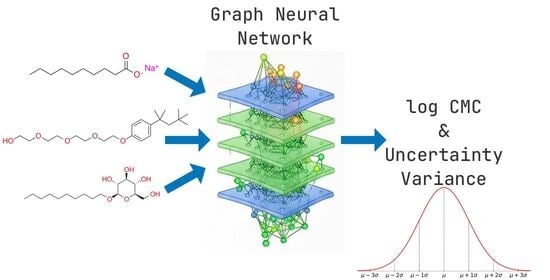
2.2. Graph Neural Network

The described model implements a hierarchical deep learning architecture for predicting CMC from molecular structures. Three GNN architectures were explored; their schematic representations are presented in Figure 1. All GNN architectures are designed to model both the target property and its predictive uncertainty [35] simultaneously. Canonical SMILES (Simplified Molecular Input Line Entry System) of surfactants get converted to molecular graphs via Chython library, version 1.78 [36], which are then passed on to MoleculeEncoder based on Graphormer principles from Chytorch, version 1.57 [37]. MoleculeEncoder is initialized with weights transferred from the rxnmap [38] pretrained model (version 1.4) of the Chytorch zoo module [28].

Molecule Encoder processes molecular graphs through atom, neighbor, and distance embeddings to generate a comprehensive 1024-dimensional representation. This representation captures complex structural and topological features through multi-head attention mechanisms within the Graphormer layer, enabling the model to discern relevant molecular patterns for CMC prediction. The general molecular representation is extracted via a Slicer operation (from Chytorch) and subsequently refined through an MLP (multilayer perceptron) with ReLU/PReLU activations. This encoder pathway effectively distills the high-dimensional graph representation into a compact, information-rich molecular fingerprint optimized for property prediction.

Molecule Encoder is the same for all architectures, but Molecular MLP in Architecture № 1 has more layers compared to Architecture № 2’s Molecular MLP because the temperature in Architecture № 2 is concatenated a few layers earlier to increase temperature values’ effect on the target property prediction, therefore better capturing the temperature–CMC relationship (Molecular MLP between architectures № 2 and № 3 remains the same).

Concurrently, the temperature input (a scalar value) is processed by a separate Temperature MLP. This network consists of three linear layers with batch normalization and PReLU activations. The number of features generated by Temperature MLP and concatenated in Concatenation MLP was calculated to account for 20% of all features.

Concatenation MLP, in Architecture № 1 and Architecture № 2, returns simultaneously a target property and uncertainty, while, in Architecture № 3, the resulting 32 features are fed into two separate MLPs, log CMC Prediction MLP and Uncertainty Prediction MLP. Target property and uncertainty prediction is split into two MLPs based on the hypothesis that independent optimization pathways would yield more precise parameter configurations for each prediction task, thereby enhancing both regression accuracy and uncertainty calibration while mitigating potential optimization conflicts between the dual objectives.

All architectures utilize progressive dropout regularization with rates decreasing from 0.3 to 0.2.

The exploration of multiple GNN architectures was systematically undertaken to identify an optimal balance between model complexity and the inherent information capacity of the single-dimensional temperature variable.

The molecular and temperature features are concatenated and fed into a final MLP that produces a two-dimensional output: the predicted log CMC value and a log-variance term. The log-variance is used to model heteroscedastic uncertainty, allowing the model to predict a confidence interval for each prediction.

Unlike uncertainty implementation in Moriarty et al.’s GNN/GP model [22], which represents a two-stage approach, our model implements an end-to-end approach where the model is trained to directly predict both CMC and uncertainty. Moriarty’s approach excels at providing theoretically sound uncertainty estimates that reflect the model’s confidence based on proximity to training data in chemical space. Our GNN model implementation described above prioritizes practical implementation and computational efficiency, directly predicting uncertainty as part of the model’s output.

This GNN model implementation utilizes transfer learning from the RxnMap model [28], which comprises two functionally distinct stages: (i) a bidirectional Graphormer molecule encoder pretrained on the PubChemQC dataset for HOMO-LUMO gap prediction, and (ii) a BERT-style network trained on reaction datasets for atom-to-atom mapping. Only the molecule encoder weights (i) were transferred to our CMC prediction model; the reaction-mapping component (ii) was excluded. This encoder possesses extensive prior knowledge of chemical space topology through its bidirectional graph transformer architecture. The encoder’s role is strictly to extract general molecular features that comprehensively represent chemical structure, while task-specific feature selection for temperature-dependent CMC prediction is delegated to subsequent MLPs. Rather than learning chemical representation de novo, the transfer learning approach effectively constrains the optimization problem to identifying the hyperplane that optimally describes log CMC property relationships within the pre-established chemical embedding space. This methodology has the potential to not only enhance model generalizability across diverse surfactant classes but also to significantly expand the applicability domain while improving prediction robustness for structurally complex molecules.

A modified loss function combining mean squared error (MSE) and uncertainty terms [35] is used in this GNN implementation:

$$L_{unc}=(1-\lambda )\cdot E\left[L\right]+\lambda \cdot E[{\displaystyle \frac{L}{{\sigma }^2}}+log({\sigma }^2\left)\right],$$

where

• L represents the base loss function (MSE in the current implementation);
• σ² denotes the predicted variance;
• $\lambda$ ∈ [0, 1] is a hyperparameter that balances the standard prediction loss and the uncertainty calibration term;
• $E[\cdot ]$ denotes the expectation over the training samples.

Parameter $\lambda$ determines how much standard MSE loss and negative log-likelihood (NLL) loss contribute to the final uncertainty. With $\lambda =1$, the model focuses entirely on aleatoric uncertainty, trained with the NLL loss for a Gaussian distribution. Aleatoric uncertainty captures noise inherent in the observations. With $\lambda =0$, modified loss is simply the mean of the base loss function. In the log CMC prediction task, aleatoric uncertainty has the potential benefit of capturing inconsistencies related to marginal differences caused by different CMC measurement methods or experimental conditions [39].

The learning procedure aims to train the prediction model such that it can estimate the predictive mean µ and variance σ² of the target property, log CMC, for each CMC measurement at a given temperature.

The GNN models are trained with AdamW optimization and a cosine annealing learning rate schedule with a warm-up of 25 epochs. Early stopping is employed to prevent overfitting. The models’ predictive performance was evaluated on external test sets from Hödl et al. [25] and Brozos et al. [24].

2.3. Performance Metrics

In this work, models’ performance was assessed with metrics such as coefficient of determination (R²), mean absolute error (MAE) and root mean squared error (RMSE).

RMSE is the square root of the average of squared prediction errors, returning the error metric to the original units of the target variable:

$$RMSE=\sqrt{{\displaystyle \frac{1}{n}}\sum _{i=1}^n{(y_i-{\widehat{y}}_i)}^2}$$

MAE measures the average absolute difference between predicted and observed values:

$$MAE={\displaystyle \frac{1}{n}}\sum _{i=1}^n\left|y_i-{\widehat{y}}_i\right|$$

The coefficient of determination, R², represents the proportion of variance in the dependent variable that is predictable from the independent variables:

$$R^2=1-{\displaystyle \frac{{\sum }_{i=1}^n{(y_i-{\widehat{y}}_i)}^2}{{\sum }_{i=1}^n{(y_i-\overline{y})}^2}}$$

Notations used in the formulas above:

• $n$ is the number of observations;
• $y_i$ represents the observed value for the i-th sample;
• ${\widehat{y}}_i$ represents the predicted value for the i-th sample;
• $\overline{y}$ is the mean of the observed values: $\overline{y}={\displaystyle \frac{1}{n}}{\sum }_{i=1}^n{y}_i$.

3. Results and Discussion

3.1. Dataset Preparation

3.1.1. General

The dataset was collected from open-access sources, which include the Qin dataset with 202 entries [21], 43 entries extracted from the Mukerjee book [40], the Chen dataset with 779 entries [26], the Hödl dataset with 1624 entries (only 1395 of which contained CMC values, and 140 of these data points were used as external test set) [25], 844 entries from the National Institute of Standards and Technology (NIST) data collection [41] and 215 data points from various sources [42,43,44,45,46,47,48,49,50]. Additionally, Brozos et al.’s (“distinct surfactants”) test set of 218 data points [24] was used as another external test set.

The collected dataset consisted of 3478 data points with SMILES of surfactants, surfactant type, measurement temperature and log CMC value (surfactant types were provided for all data points except those extracted from the Mukerjee book, the NIST data collection and Brozos et al., for which surfactant types were manually assigned based on examination of molecular structures). All CMC values were reported in logarithmic form (log CMC mol/L); values provided in other units were converted to log CMC prior to inclusion in the dataset. Data points with missing temperature values were discarded during processing.

Two external test sets were used in this work:

• Hödl et al.’s test set [25] comprised 140 data points (for assessing CMC prediction accuracy across all surfactant types, including gemini surfactants, log CMC values range from −0.5 to −6.0 and molecular masses range between 174 and 1196 g/mol);
• Brozos et al’s. test set [24] comprised 218 data points (for assessing CMC’s temperature dependency across multiple surfactant types, log CMC values range from 0.2 to −4.7 and molecular masses are between 90 and 663 g/mol).

The procedure of data preprocessing included the following steps:

• Chemical structure canonicalization: SMILES were canonicalized using the canonicalize method of MoleculeContainer from Chython library. Separately canonicalization using “canonicalize” and “clean_stereo” methods was performed for inspecting different stereoisomers. Stereoisomers without provided anomeric configuration or stereo features were dropped.
• Exact duplicates—defined as identical SMILES, temperature and log CMC values—were removed to prevent overrepresentation in the dataset. Generally, primary sources were prioritized over aggregated literature sources and datasets. Surfactants with multiple measurements at the same temperature were manually examined, and the log CMC values were averaged (“CMC_average”) if the range (Δlog CMC) between the maximum and minimum values was ≤0.01; in other cases, values from less trusted sources were deleted.
• Temperature dependency of each surfactant was manually analyzed by plotting log CMC [mol/L] against temperature [°C]. Measurements significantly deviating from monotonic or U-shaped relationships were removed from the dataset (temperature dependency plots of surfactants in the final dataset are presented in Section 3.1.2).
• Verification of data accuracy through original source: For duplicate entries—defined as identical SMILES and temperature values—present across multiple datasets with conflicting log CMC values, the original cited sources were consulted to verify and select the most accurate and consistent values, ensuring fidelity to the primary experimental data.
• Manual inspection of molecular structures: A final visual audit of all structures was conducted to detect anomalies; any suspicious entries were verified and corrected by consulting the original source literature. Unresolved cases were excluded to ensure structural accuracy and dataset integrity.

Entries from the NIST data collection [41] were separately filtered out based on SMILES inspection and the measurement method, prioritizing tensiometry and conductivity-based methods as opposed to other methods (consistent with the data acquisition approach reported by Hödl et al. [25]).

The final processed dataset excluded all external test set compounds. The resulting dataset after general preparations contains 2133 log CMC values with associated temperatures for 1815 unique surfactants. The complete curated dataset is provided in the Supplementary Materials.

3.1.2. Temperature

The distribution of measurement temperatures for the CMC in the processed dataset is shown in Figure 2. The majority of measurements were conducted at 25 °C, accounting for ~72% of the data. Temperatures below and above 25 °C made up ~7% and ~21% of all measurements, respectively. This distribution highlights preference for measurements near room temperature, particularly at 25 °C, with limited data available at other temperatures.

Examples of temperature–CMC relationships from the final dataset and their plots are presented in Figure 3: U-shaped relationships for cationic and anionic surfactants with a minimum log CMC at 30 °C and 45 °C, respectively, and a U-shaped relationship for sugar-based surfactants with a minimum at 45 °C, monotonically decreasing for nonionic ones with a minimum at 40 °C and non-monotonic for zwitterionic ones with a maximum at 35 °C.

3.1.3. Molecular Mass

Molecular mass values were calculated using the “molecular_mass” property of “MoleculeContainer” from Chython using canonical SMILES of surfactants.

The present distribution in Figure 4 highlights the scarcity of high-mass surfactants. Consequently, structures exceeding ~1098 g/mol were excluded from the log CMC modeling dataset due to their scarcity (representing <1% of curated surfactant entries). This curation step ensured the model’s robustness and applicability to industrially significant surfactant design spaces. Removal also eliminated outliers that would distort model robustness and shifted the molecular mass distribution toward a more Gaussian-like profile (though moderately left-skewed), with the mean mass converging at approximately 500 g/mol. A molecular mass distribution histogram of the final dataset is shown in Figure 5.

The resulting processed dataset contains 2133 log CMC values with associated temperatures for 1815 unique surfactants.

3.1.4. Surfactant Type

The processed dataset included 1815 surfactants, among which 438 were gemini cationic surfactants, 417 were nonionic surfactants, 377 were anionic surfactants, 361 were cationic surfactants, 153 were sugar-based nonionic surfactants, 58 were zwitterionic surfactants, 10 were gemini zwitterionic surfactants and 1 was a gemini anionic surfactant (Figure 6).

The histogram plot (Figure 7) illustrates the distribution of critical micelle concentration (log CMC, mol/L) values for five major surfactant classes—nonionic (includes Sugar-based surfactants), cationic, anionic, zwitterionic and gemini (includes gemini anionic, gemini cationic and gemini zwitterionic)—with the full processed dataset distribution represented as a gray contour line and the overall median indicated by a dashed black line. Lower (<−5 log CMC) and higher (<−1 log CMC) value CMC measurements appear to be less prevalent for all major surfactant types. Zwitterionic surfactants, being the least presented surfactant type, have the fewest CMC measurements.

3.2. Training and Validation Set Preparation

To eliminate potential data leakage, the entire dataset was checked for the presence of any data points from the external test sets from Hödl et al. [25] and Brozos et al. [24] by comparing canonicalized SMILES. The final processed dataset comprised 2133 data points, excluding the Hödl external test set consisting of 140 data points and the Brozos external test set of 218 data points.

The prepared dataset was split into train and validation sets. The validation set of 200 entries (~9% of the total) was prepared in two steps: (1) a single data point was randomly selected from each surfactant with multiple measurements (≥5 measurements—to keep as much temperature-dependency data in the training data as possible) at different temperatures; (2) data points were selected proportionally by category frequency from surfactants with single data point present in the dataset. The train set included 1933 data points.

Around half of the data points in the validation set originally were sourced from the Hödl et al. dataset, with 25% from the Chen et al. dataset; ~70% of the validation set points were at 25 °C, ~7% were below 25 °C and ~24% were above 25 °C.

3.3. Modeling

3.3.1. Predictive Performance of RF and XGB Models

This study employs Bayesian optimization via Optuna [51], version 4.5.0, to minimize cross-validated RMSE for regression models applied to molecular fingerprint data. Both XGB and RF models are run for 100 trials to converge toward optimal solutions while minimizing over-optimization risk through 5-fold CV with enabled shuffling. Overall, 1933 data points of the train set were utilized for performing cross-validation. During cross-validation, data partitioning ensured each sample appeared exactly once in the test fold across all folds, per standard k-fold CV practice.

For Random Forest, optimization centered on tree complexity control and feature subsampling tailored to fingerprint dimensionality:

• max_features explored fractional (0.1–0.5) values and heuristics (“sqrt”, “log2”);
• max_depth explicitly included None (unconstrained trees) and values between 10 and 50 to evaluate depth necessity;
• min_samples_split (2–20);
• min_samples_leaf (1–15);
• n_estimators used log-scale sampling (100–1000);
• bootstrap parameters (max_samples, 0.5–1.0) were conditionally optimized only with enabled bootstrap.

For XGBoost, the search prioritized regularization and subsampling parameters. Key constraints reflect domain knowledge:

• max_depth was restricted to values between 3 and 10 to model chemical relationships without overfitting;
• colsample_bytree (0.3–0.7) and subsample (0.6–0.95) mitigated feature redundancy;
• reg_alpha and reg_lambda were explored over 10⁻⁸ to 10.0 with log-uniform sampling, ensuring robust exploration of orders-of-magnitude effects;
• tree_method “hist” ensured computational efficiency for large feature spaces.

RF’s best trial achieved a CV result of RMSE = 0.651 with the following set of parameters: max_features = 0.2, max_depth = 30, min_samples_split = 3, min_samples_leaf = 1, n_estimators = 846, bootstrap = False. XGB’s best trial achieved a CV result of RMSE = 0.650 with this set of parameters: max_depth = 9, min_child_weight = 9, subsample = 0.859, colsample_bytree = 0.528, reg_alpha = 1.693 × 10⁻⁵, reg_lambda = 3.016 × 10⁻³, learning_rate = 0.110, gamma = 6.618 × 10⁻³.

All of the metrics for XGB and RF models tested on the external test sets are presented in

Table 1. Performance metrics on the external test sets (Hödl et al. [25] and Brozos et al. [24] test set) for optimized fingerprint-based models.

Models	Test Set	R2	MAE	RMSE
RF	Hödl et al. Test Set	0.695	0.393	0.592
XGB	Hödl et al. Test Set	0.677	0.390	0.608
RF	Brozos et al. Test Set	0.727	0.402	0.541
XGB	Brozos et al. Test Set	0.778	0.372	0.488

. Among the tested models, the XGBoost Regressor achieved the highest predictive performance on the Brozos et al. external test set with R² of 0.778 and RMSE of 0.488, and Random Forest Regressor achieved better predictive performance on the Hödl et al. external test set with R² of 0.695 and RMSE of 0.592.

3.3.2. Predictive Performance of GNN Models and Comparison with Previous Studies

After establishing a baseline result with the fingerprint-based models, proposed GNN models were trained on the train set of 1933 data points and validation set of 200 data points (partitioning method is described in Section 3.2). Each model was trained in ~150 epochs with early stopping whilst monitoring the validation set RMSE value. The uncertainty training parameter $\lambda$ described in Section 2.2 was set to 1; we found that other $\lambda$ values, such as 0.1 and 0, yielded weak Spearman rank correlation ρ and poor calibration compared to models trained with $\lambda =1$. Training data R² and RMSE were around 0.96 and 0.24, respectively. The most optimal model for each of the proposed architectures was selected based on the validation set RMSE value. The predictive ability of the trained models was tested on the same external test sets as the fingerprint-based models (Section 3.3.1).

The GNN models developed in this study attained relatively similar performance on each test set (all metrics are reported in

Table 2. Performance metrics on the external test sets (Hödl et al. [25] and Brozos et al. [24]) for the trained GNN models and models by Hödl et al. and Brozos et al. for comparison.

Models	Hödl et al. Test Set				Brozos et al. Test Set
	R2	MAE	RMSE	Spearman ρ	R2	MAE	RMSE	Spearman ρ
GNN Architecture № 1	0.890	0.230	0.355	0.238	0.868	0.255	0.375	0.227
GNN Architecture № 2	0.882	0.241	0.367	0.177	0.850	0.278	0.401	0.377
GNN Architecture № 3	0.877	0.240	0.376	0.230	0.892	0.225	0.340	0.345
Hödl et al. (2025) single-property model *	–	0.241	0.365	–	–	–	–	–
Brozos et al. (2024) model	–	–	–	–	0.95	0.15	0.24	–

* Coefficient of determination R² was not reported by Hödl et al.

). All GNN models demonstrate superior predictive performance for the target property compared to fingerprint-based RF and XGB baselines (Table 1). The best performance on Hödl et al.’s test set was achieved by the GNN model with Architecture № 1, while better performance on Brozos et al.’s test set was achieved with Architecture № 3. This is explained by the fact that most of the data entries in train and validation sets were originally sourced from the Hödl et al. dataset. Therefore, model optimization for temperature-dependent predictions that are present in the Brozos et al. test set will inevitably lead to a slight decrease in the performance on the Hödl et al. test set. Uncertainty prediction analysis is discussed in Section 4.

To ensure methodological consistency in evaluating single-property prediction capability, comparisons were restricted to single-property models from Hödl et al. [25]. Multi-property prediction models (i.e., those leveraging γ_CMC, Г_max × 10⁶ and pC₂₀ property values, alongside pCMC) inherently benefit from expanded datasets during training. Consequently, our GNN was benchmarked against the single-property model of Hödl et al. [25] on their external test set.

Proposed GNN architectures performed similarly compared to Hödl et al.’s single-property prediction model. However, Brozos et al.’s model demonstrates significantly better performance due to the richer temperature-dependency information present in their proprietary dataset compared to our dataset collected from open sources.

Temperature relationship plot analysis for predicted values (Figure 8) reveals that Architecture № 1 was able to capture only monotonically increasing relationships or non-monotonic relationships with a CMC maximum at 30–40 °C. Earlier concatenation of temperature features in Architectures № 2 and № 3 appears to have benefited both performance metrics and allowed us to capture U-shaped (Figure 8a,b) and monotonically decreasing (Figure 8c) relationships. However, the predicted curve for zwitterionic surfactants (Figure 8d) does not replicate the experimental relationship, but the predicted values remain close to the experimentally observed data points. Overall, the attained results demonstrate that earlier concatenation of temperature in Architectures № 2 and № 3 noticeably benefits model’s ability to capture temperature dependence (this result also aligns with the findings of Brozos et al. [24]).

4. GNN Model Uncertainty Prediction Analysis

Uncertainty quantification performance was evaluated in terms of the Spearman rank correlation coefficient ρ between the absolute prediction error and uncertainty score on the test set—the methodology consistent with [35]. Between correlation coefficients of two test sets, GNN Architecture № 3 demonstrated the best overall performance, even though correlation on individual test sets was higher for other architectures (Spearman ρ values for each GNN architecture are displayed in Table 2).

We consider a correlation of 0.3 to be high in this context, as a substantially higher Spearman correlation would typically imply that the model could achieve more accurate point predictions of the target property. Moreover, the observed level of correlation supports the model’s ability to reflect not only its own predictive uncertainty but also the inherent variability and potential experimental error present in the measured CMC values.

GNN models’ uncertainty quantification approximately follows the normal distribution (the actual predicted uncertainty distribution is shown in Figure 9), showing strong calibration at high confidence thresholds, with near-ideal coverage for both 2σ (94.95% vs. target 95.45%) and 3σ intervals (97.71% vs. target 99.73%) and slightly higher coverage at the 1σ level (74.77% coverage vs. 68.27% theoretical). Overall, the model’s uncertainty estimates are reasonably well-calibrated and a similar relationship is observed for other GNN architectures.

Additionally, scatter plots for the proposed GNN models (scatter plot for Architecture № 2 is presented in Figure 10) reveal an interesting relationship—a lower predicted log CMC value generally coincides with a higher predicted uncertainty. This trend is visually evident in the increasing spread of prediction intervals (“whiskers”) at lower log CMC values, likely reflecting the fact that lower CMC values are less represented in the dataset (Figure 7). Higher uncertainty values may also be caused by the particular method’s detection limits at lower CMC measurements.

5. Conclusions

Data from multiple sources was united into a curated comprehensive dataset of 2133 CMC values with associated measurement temperatures. Uncertainty-aware GNN combines high-precision log CMC prediction with built-in uncertainty quantification, delivering both accurate point estimates and well-calibrated uncertainty estimates in a single forward pass. Future work should prioritize dataset expansion for underrepresented surfactant classes (e.g., zwitterionics) and broader temperature coverage beyond the predominant 25 °C measurements. Uncertainty quantification could be further refined by explicitly modeling the measurement method as an aleatoric uncertainty source. Architectural improvements—such as cross-attention or gated fusion mechanisms—could better capture complex temperature–structure interactions, while class-balanced oversampling (e.g., synthetic minority oversampling technique) and ensemble techniques may enhance robustness for minority classes, ultimately yielding a more universally applicable CMC prediction framework.

References

1. Turchi, M.; Karcz, A.P.; Andersson, M.P. First-Principles Prediction of Critical Micellar Concentrations for Ionic and Nonionic Surfactants. J. Colloid Interface Sci. 2022, 606, 618–627. [Google Scholar] [CrossRef] [PubMed]
2. Cárdenas, H.; Kamrul-Bahrin, M.A.H.; Seddon, D.; Othman, J.; Cabral, J.T.; Mejía, A.; Shahruddin, S.; Matar, O.K.; Müller, E.A. Determining Interfacial Tension and Critical Micelle Concentrations of Surfactants from Atomistic Molecular Simulations. J. Colloid Interface Sci. 2024, 674, 1071–1082. [Google Scholar] [CrossRef]
3. Mattei, M.; Kontogeorgis, G.M.; Gani, R. Modeling of the Critical Micelle Concentration (CMC) of Nonionic Surfactants with an Extended Group-Contribution Method. Ind. Eng. Chem. Res. 2013, 52, 12236–12246. [Google Scholar] [CrossRef]
4. Smith, C.; Lu, J.R.; Thomas, R.K.; Tucker, I.M.; Webster, J.R.P.; Campana, M. Markov Chain Modeling of Surfactant Critical Micelle Concentration and Surface Composition. Langmuir 2019, 35, 561–569. [Google Scholar] [CrossRef]
5. Sanchez-Lengeling, B.; Aspuru-Guzik, A. Inverse Molecular Design Using Machine Learning: Generative Models for Matter Engineering. Science 2018, 361, 360–365. [Google Scholar] [CrossRef]
6. Afonina, V.A.; Mazitov, D.A.; Nurmukhametova, A.; Shevelev, M.D.; Khasanova, D.A.; Nugmanov, R.I.; Burilov, V.A.; Madzhidov, T.I.; Varnek, A. Prediction of Optimal Conditions of Hydrogenation Reaction Using the Likelihood Ranking Approach. Int. J. Mol. Sci. 2021, 23, 248. [Google Scholar] [CrossRef]
7. Albrijawi, M.T.; Alhajj, R. LSTM-Driven Drug Design Using SELFIES for Target-Focused de Novo Generation of HIV-1 Protease Inhibitor Candidates for AIDS Treatment. PLoS ONE 2024, 19, e0303597. [Google Scholar] [CrossRef]
8. Bushuev, K.R.; Lobanov, I.S. Machine Learning Method for Computation of Optimal Transitions in Magnetic Nanosystems. Nanosyst. Physics Chem. Math. 2020, 11, 642–650. [Google Scholar] [CrossRef]
9. Huibers, P.D.T.; Lobanov, V.S.; Katritzky, A.R.; Shah, D.O.; Karelson, M. Prediction of Critical Micelle Concentration Using a Quantitative Structure-Property Relationship Approach. 1. Nonionic Surfactants. Langmuir 1996, 12, 1462–1470. [Google Scholar] [CrossRef]
10. Huibers, P.D.T.; Lobanov, V.S.; Katritzky, A.R.; Shah, D.O.; Karelson, M. Prediction of Critical Micelle Concentration Using a Quantitative Structure–Property Relationship Approach. 2. Anionic Surfactants. J. Colloid Interface Sci. 1997, 187, 113–120. [Google Scholar] [CrossRef]
11. Li, X.; Zhang, G.; Dong, J.; Zhou, X.; Yan, X.; Luo, M. Estimation of Critical Micelle Concentration of Anionic Surfactants with QSPR Approach. J. Mol. Struct. THEOCHEM 2004, 710, 119–126. [Google Scholar] [CrossRef]
12. Wang, Z.; Huang, D.; Gong, S.; Li, G. Prediction on Critical Micelle Concentration of Nonionic Surfactants in Aqueous Solution: Quantitative Structure-Property Relationship Approach. Chin. J. Chem. 2003, 21, 1573–1579. [Google Scholar] [CrossRef]
13. Katritzky, A.R.; Pacureanu, L.; Dobchev, D.; Karelson, M. QSPR Study of Critical Micelle Concentration of Anionic Surfactants Using Computational Molecular Descriptors. J. Chem. Inf. Model. 2007, 47, 782–793. [Google Scholar] [CrossRef]
14. Jiao, L.; Wang, Y.; Qu, L.; Xue, Z.; Ge, Y.; Liu, H.; Lei, B.; Gao, Q.; Li, M. Hologram QSAR Study on the Critical Micelle Concentration of Gemini Surfactants. Colloids Surf. A Physicochem. Eng. Asp. 2020, 586, 124226. [Google Scholar] [CrossRef]
15. Creton, B.; Barraud, E.; Nieto-Draghi, C. Prediction of Critical Micelle Concentration for Per- and Polyfluoroalkyl Substances. SAR QSAR Environ. Res. 2024, 35, 309–324. [Google Scholar] [CrossRef]
16. Anoune, N.; Nouiri, M.; Berrah, Y.; Gauvrit, J.; Lanteri, P. Critical Micelle Concentrations of Different Classes of Surfactants: A Quantitative Structure Property Relationship Study. J. Surfactants Deterg. 2002, 5, 45–53. [Google Scholar] [CrossRef]
17. Rahal, S.; Hadidi, N.; Hamadache, M. In Silico Prediction of Critical Micelle Concentration (CMC) of Classic and Extended Anionic Surfactants from Their Molecular Structural Descriptors. Arab. J. Sci. Eng. 2020, 45, 7445–7454. [Google Scholar] [CrossRef]
18. Laidi, M.; Abdallah, E.; Si-Moussa, C.; Benkortebi, O.; Hentabli, M.; Hanini, S. CMC of Diverse Gemini Surfactants Modelling Using a Hybrid Approach Combining SVR-DA. Chem. Ind. Chem. Eng. Q. 2021, 27, 299–312. [Google Scholar] [CrossRef]
19. Soria-Lopez, A.; García-Martí, M.; Barreiro, E.; Mejuto, J.C. Ionic Surfactants Critical Micelle Concentration Prediction in Water/Organic Solvent Mixtures by Artificial Neural Network. Tenside Surfactants Deterg. 2024, 61, 519–529. [Google Scholar] [CrossRef]
20. Boukelkal, N.; Rahal, S.; Rebhi, R.; Hamadache, M. QSPR for the Prediction of Critical Micelle Concentration of Different Classes of Surfactants Using Machine Learning Algorithms. J. Mol. Graph. Model. 2024, 129, 108757. [Google Scholar] [CrossRef]
21. Qin, S.; Jin, T.; Lehn, R.C.V.; Zavala, V.M. Predicting Critical Micelle Concentrations for Surfactants Using Graph Convolutional Neural Networks. J. Phys. Chem. B 2021, 125, 10610–10620. [Google Scholar] [CrossRef]
22. Moriarty, A.; Kobayashi, T.; Salvalaglio, M.; Striolo, A.; McRobbie, I. Analyzing the Accuracy of Critical Micelle Concentration Predictions Using Deep Learning. J. Chem. Theory Comput. 2023, 19, 7371–7386. [Google Scholar] [CrossRef] [PubMed]
23. Theis Marchan, G.; Balogun, T.O.; Territo, K.; Das, D.; Olayiwola, T.; Kumar, R.; Romagnoli, J.A. Toward Harnessing AI for Surfactant Chemistry: Prediction of Critical Micelle Concentration. Comput. Mater. Sci. 2026, 265, 114548. [Google Scholar] [CrossRef]
24. Brozos, C.; Rittig, J.G.; Bhattacharya, S.; Akanny, E.; Kohlmann, C.; Mitsos, A. Predicting the Temperature Dependence of Surfactant CMCs Using Graph Neural Networks. J. Chem. Theory Comput. 2024, 20, 5695–5707. [Google Scholar] [CrossRef]
25. Hödl, S.L.; Hermans, L.; Dankloff, P.F.J.; Piruska, A.; Huck, W.T.S.; Robinson, W.E. SurfPro—A Curated Database and Predictive Model of Experimental Properties of Surfactants. Digit. Discov. 2025, 4, 1176–1187. [Google Scholar] [CrossRef]
26. Chen, J.; Hou, L.; Nan, J.; Ni, B.; Dai, W.; Ge, X. Prediction of Critical Micelle Concentration (CMC) of Surfactants Based on Structural Differentiation Using Machine Learning. Colloids Surf. A Physicochem. Eng. Asp. 2024, 703, 135276. [Google Scholar] [CrossRef]
27. Barbosa, G.D.; Striolo, A. Machine Learning Prediction of Critical Micellar Concentration Using Electrostatic and Structural Properties as Descriptors. J. Chem. Eng. Data 2025, 70, 4019–4030. [Google Scholar] [CrossRef]
28. Nugmanov, R.; Dyubankova, N.; Gedich, A.; Wegner, J.K. Bidirectional Graphormer for Reactivity Understanding: Neural Network Trained to Reaction Atom-to-Atom Mapping Task. J. Chem. Inf. Model. 2022, 62, 3307–3315. [Google Scholar] [CrossRef] [PubMed]
29. Fallani, A.; Nugmanov, R.; Arjona-Medina, J.; Wegner, J.K.; Tkatchenko, A.; Chernichenko, K. Pretraining Graph Transformers with Atom-in-a-Molecule Quantum Properties for Improved ADMET Modeling. J. Cheminform. 2025, 17, 25. [Google Scholar] [CrossRef]
30. Arjona-Medina, J.; Nugmanov, R. Analysis of Atom-Level Pretraining with Quantum Mechanics (QM) Data for Graph Neural Networks Molecular Property Models. arXiv 2024, arXiv:2405.14837. [Google Scholar] [CrossRef]
31. Saifullin, E.R.; Gimadiev, T.R.; Khakimova, A.A.; Varfolomeev, M.A. Game Changer in Chemical Reagents Design for Upstream Applications: From Long-Term Laboratory Studies to Digital Factory Based On AI. In Proceedings of the Abu Dhabi International Petroleum Exhibition and Conference (ADIPEC), Abu Dhabi, United Arab Emirates, 4–7 November 2024; p. D031S088R006. [Google Scholar]
32. RDKit. Available online: https://www.rdkit.org/ (accessed on 18 November 2025).
33. Pedregosa, F.; Varoquaux, G.; Gramfort, A.; Michel, V.; Thirion, B.; Grisel, O.; Blondel, M.; Prettenhofer, P.; Weiss, R.; Dubourg, V.; et al. Scikit-Learn: Machine Learning in Python. J. Mach. Learn. Res. 2011, 12, 2825–2830. [Google Scholar]
34. XGBoost Python Package—Xgboost 3.0.5 Documentation. Available online: https://xgboost.readthedocs.io/en/release_3.0.0/python/index.html (accessed on 18 November 2025).
35. Kwon, Y. Uncertainty-Aware Prediction of Chemical Reaction Yields with Graph Neural Networks. J. Cheminform. 2022, 14, 2. [Google Scholar] [CrossRef]
36. Chython/Chython. Available online: https://github.com/chython/chython (accessed on 18 November 2025).
37. Chython/Chytorch. Available online: https://github.com/chython/chytorch (accessed on 18 November 2025).
38. Chython/Chytorch-Rxnmap. Available online: https://github.com/chython/chytorch-rxnmap (accessed on 18 November 2025).
39. Scholz, N.; Behnke, T.; Resch-Genger, U. Determination of the Critical Micelle Concentration of Neutral and Ionic Surfactants with Fluorometry, Conductometry, and Surface Tension—A Method Comparison. J. Fluoresc. 2018, 28, 465–476. [Google Scholar] [CrossRef]
40. Mukerjee, P.; Mysels, K. Critical Micelle Concentrations of Aqueous Surfactant Systems; National Bureau of Standards: Gaithersburg, MD, USA, 1971; p. NBS NSRDS 36. [Google Scholar]
41. Frey, J.G.; Pearman-Kanza, S.; Munday, S. Critical Micelle Concentration (CMC) Data Collection. Available online: https://resources.psdi.ac.uk/data/a7c82670-d2e2-46c6-920a-74294289aa34 (accessed on 30 December 2025).
42. Perger, T.-M.; Bešter-Rogač, M. Thermodynamics of Micelle Formation of Alkyltrimethylammonium Chlorides from High Performance Electric Conductivity Measurements. J. Colloid Interface Sci. 2007, 313, 288–295. [Google Scholar] [CrossRef] [PubMed]
43. Galgano, P.D.; El Seoud, O.A. Micellar Properties of Surface Active Ionic Liquids: A Comparison of 1-Hexadecyl-3-Methylimidazolium Chloride with Structurally Related Cationic Surfactants. J. Colloid Interface Sci. 2010, 345, 1–11. [Google Scholar] [CrossRef]
44. Angarten, R.G.; Loh, W. Thermodynamics of Micellization of Homologous Series of Alkyl Mono and Di-Glucosides in Water and in Heavy Water. J. Chem. Thermodyn. 2014, 73, 218–223. [Google Scholar] [CrossRef]
45. Cheng, C.; Qu, G.; Wei, J.; Yu, T.; Ding, W. Thermodynamics of Micellization of Sulfobetaine Surfactants in Aqueous Solution. J. Surfactants Deterg. 2012, 15, 757–763. [Google Scholar] [CrossRef]
46. González-Pérez, A.; Ruso, J.M.; Romero, M.J.; Blanco, E.; Prieto, G.; Sarmiento, F. Application of Thermodynamic Models to Study Micellar Properties of Sodium Perfluoroalkyl Carboxylates in Aqueous Solutions. Chem. Phys. 2005, 313, 245–259. [Google Scholar] [CrossRef]
47. Blanco, E.; González-Pérez, A.; Ruso, J.M.; Pedrido, R.; Prieto, G.; Sarmiento, F. A Comparative Study of the Physicochemical Properties of Perfluorinated and Hydrogenated Amphiphiles. J. Colloid Interface Sci. 2005, 288, 247–260. [Google Scholar] [CrossRef]
48. Meguro, K.; Takasawa, Y.; Kawahashi, N.; Tabata, Y.; Ueno, M. Micellar Properties of a Series of Octaethyleneglycol-n-Alkyl Ethers with Homogeneous Ethylene Oxide Chain and Their Temperature Dependence. J. Colloid Interface Sci. 1981, 83, 50–56. [Google Scholar] [CrossRef]
49. Castro, G.; Garrido, P.F.; Amigo, A.; Brocos, P. Boosting the Use of Thermoacoustimetry in Micellization Thermodynamics Studies by Easing an Objective Determination of the Cmc. Fluid Phase Equilibria 2018, 478, 1–13. [Google Scholar] [CrossRef]
50. Eggenberger, D.N.; Harwood, H.J. Conductometric Studies of Solubility and Micelle Formation1. J. Am. Chem. Soc. 1951, 73, 3353–3355. [Google Scholar] [CrossRef]
51. Akiba, T.; Sano, S.; Yanase, T.; Ohta, T.; Koyama, M. Optuna: A Next-Generation Hyperparameter Optimization Framework. In Proceedings of the 25th ACM SIGKDD International Conference on Knowledge Discovery & Data Mining, Anchorage, AK, USA, 4–8 August 2019; Association for Computing Machinery: New York, NY, USA, 2019. [Google Scholar]
Figure 1. Proposed GNN model architecture variants implementing hierarchical deep learning approach: GNN Architecture № 1 with simplest structure predicting both target property and its uncertainty, GNN Architecture № 2 concatenating temperature earlier in the hierarchy compared to Architecture № 1 to increase temperature’s influence on the target property prediction, and GNN Architecture № 3 splitting target property and uncertainty prediction into separate MLPs for better weight optimization. Red font color indicates temperature-derived features from the Temperature MLP are incorporated into the Concatenation MLP.
Chemistry 08 00026 g001
Figure 2. The distribution of temperature in the final dataset (2133 data points) excluding the external test sets. The Y axis is displayed in logarithmic scale.
Chemistry 08 00026 g002
Figure 3. Log CMC temperature dependency plots for cationic (a), anionic (b), nonionic (c), zwitterionic (d) and sugar-based nonionic (e,f) surfactants present in the final dataset.
Chemistry 08 00026 g003
Figure 4. Molecular mass distribution of the processed dataset before removal by ~1098 g/mol upper bound.
Chemistry 08 00026 g004
Figure 5. Molecular mass distribution of the final dataset (2133 data points) after removing data points with molecular mass greater than ~1098 g/mol.
Chemistry 08 00026 g005
Figure 6. The distribution of surfactant types in the processed dataset of 2133 data entries.
Chemistry 08 00026 g006
Figure 7. Distribution of log CMC values for major surfactant categories in the processed dataset, with gemini surfactants of all charge types (cationic, anionic, zwitterionic) placed into a single “Gemini” category. The gray contour line represents the log CMC distribution of the complete dataset of 2133 data points for reference. Overall log CMC median = −3.0. Log CMC median of each surfactant type is represented with dashed line of corresponding color (blue for nonionic, orange for gemini, green for cationic, red for anionic and purple for zwitterionic).
Chemistry 08 00026 g007
Figure 8. Log CMC versus temperature plots for observed (blue dots) and predicted (red squares) values for nonionic (a), anionic (b), cationic (c) and zwitterionic (d) surfactants. Predicted uncertainty (±1σ) is represented with the red background. Results are shown for three GNN architectures (№ 1, № 2, № 3), with each column corresponding to one architecture.
Chemistry 08 00026 g008
Figure 9. Coverage of prediction intervals compared to theoretical coverage under a normal (Gaussian) distribution. The blue solid line shows the percentage of true values falling within predicted intervals of width ±kσ (where k = 0 to 3), based on empirical evaluation across the test set. The red dashed line represents the expected coverage under an ideal Gaussian distribution. Vertical green dashed lines mark ±1σ, ±2σ, and ±3σ thresholds.
Chemistry 08 00026 g009
Figure 10. Scatter plots of values predicted using GNN Architecture № 2 versus true log CMC values: (a) Brozos et al. (2024) [24] external test set (218 data points), R2 = 0.850; (b) Hödl et al. (2025) [25] external test set (140 data points), R2 = 0.882. The red dashed line serves as a visual reference for perfect agreement between predicted and experimental log CMC values.
Chemistry 08 00026 g010