Image-Based Multi-Domain Feature Extraction for IoUT-Oriented Monitoring of Hydrofoil Tip Leakage Flow Cavitation

Abstract

For Internet of Underwater Things (IoUT)−oriented condition monitoring of underwater propulsion systems, continuous visual observations can provide rich information on the spatial distribution and temporal evolution of cavitation, while the direct transmission of complete image sequences may impose a substantial data burden on underwater communication networks. To provide compact and physically interpretable visual monitoring information, this study develops an image-derived multi-domain feature−extraction method for hydrofoil cavitation monitoring. Cavitation image sequences of an original NACA0009 hydrofoil and a hydrofoil with hole−pit structures were analyzed as two experimental configurations exhibiting different cavitation behaviors. Static−background subtraction, RGB−channel−response processing, Canny edge detection, morphological processing, and threshold-based focusing were applied to extract cavitation regions. The normalized cavitation−area time series of the tip leakage vortex (TLV), tip separation vortex (TSV), and six local regions were then constructed from consecutive images and treated as image-derived monitoring signals. Time−domain and spatial features were used to characterize the overall cavitation level and regional distribution, while Fast Fourier Transform (FFT) and Discrete Wavelet Transform (DWT) were further employed to describe spectral fluctuations and multi-scale transient variations. The extracted monitoring features showed clear responses to changes in hydrofoil configuration and operating conditions. Under the baseline condition, the mean TLV and TSV cavitation−area features of the hydrofoil with hole−pit structures were approximately 40.0% and 85.0% lower than those of the original hydrofoil, respectively. Differences were also observed in the regional, frequency−domain, and time−frequency characteristics and remained observable under the two changed operating conditions. These results indicate that continuous cavitation images can be transformed into complementary multi-domain descriptors for characterizing variations in cavitation behavior. The proposed approach therefore provides a potential visual sensing and feature−extraction component for future IoUT-based condition monitoring of underwater propulsion systems, while reducing reliance on the transmission of complete image sequences.

1. Introduction

1.1. Background and Motivation

Cavitation is an important unsteady phenomenon associated with underwater propulsion components. In components with finite tip clearance, the pressure difference between the pressure and suction sides generates tip leakage flow and complex vortex structures, including the tip leakage vortex (TLV) and tip separation vortex (TSV). Low-pressure regions within these vortical structures may induce cavitation, which is associated with energy loss, performance degradation, vibration, hydrodynamic noise, and material erosion [1,2,3,4,5]. Previous studies have investigated various passive and active approaches for modifying tip leakage flow and suppressing cavitation [1,2,6,7,8,9,10,11,12,13,14,15,16,17]. In addition to the hydrodynamic mechanisms and suppression effects, however, the occurrence, extent, spatial distribution, and temporal evolution of cavitation also provide observable information that can be used for cavitation monitoring and may support the future development of cavitation−detection methods.

High-speed imaging provides a direct and non-intrusive means of recording the dynamic evolution of cavitation. Consecutive cavitation images preserve not only the spatial morphology and distribution of cavitation structures but also their temporal variations during development, migration, shedding, and collapse. Compared with isolated images or time-averaged quantities, continuous image sequences therefore contain richer information for characterizing whether and how cavitation behavior changes over time. If such visual information can be further converted into quantitative and machine-readable descriptors, it can provide a basis for image-based cavitation monitoring and may also support the future development of autonomous cavitation−detection methods for underwater propulsion components.

The Internet of Underwater Things (IoUT) provides a potential framework for connecting underwater sensing, information processing, communication, and remote monitoring [18,19,20,21,22,23]. Compared with conventional terrestrial IoT systems, underwater communication is more strongly constrained by limited bandwidth, long propagation delays, unstable transmission channels, and energy consumption. These limitations become particularly important when visual information is considered, because continuous high-resolution or high-speed image sequences generally contain much larger amounts of data than conventional scalar sensing signals. Therefore, directly transmitting complete cavitation image sequences is not necessarily suitable for continuous IoUT-oriented monitoring.

A more practical approach is to extract useful monitoring information from the image sequences before subsequent transmission or analysis. Frame-by-frame cavitation characteristics can be converted into temporally connected image-derived signals, thereby retaining information on cavitation behavior without relying solely on complete raw image sequences. For example, cavitation−area signals can describe variations in the overall cavitation level, measurements from different regions can represent spatial differences, and frequency−domain and time−frequency characteristics can provide additional information on periodic fluctuations and transient variations. From this perspective, the key issue is how to transform continuous cavitation images into compact, quantitative, and physically interpretable descriptors that remain sensitive to changes in cavitation behavior.

Accordingly, the present study focuses on the visual−information processing stage that could support future IoUT-based cavitation monitoring and autonomous detection. Rather than developing a complete IoUT communication architecture, the study investigates how continuous high-speed cavitation images can be converted into image-derived monitoring signals and subsequently characterized from temporal, spatial, frequency−domain, and time−frequency perspectives. Such a representation is intended to provide a methodological basis for extracting useful cavitation information from visual observations and for its potential integration into future monitoring and autonomous−detection systems for underwater propulsion components.

1.2. State of the Art in IoUT-Oriented Cavitation Monitoring

Research related to the present study mainly involves three interconnected areas: IoUT-oriented underwater monitoring, image-based cavitation observation and quantification, and multi-domain feature extraction from continuous cavitation images. IoUT research provides the framework for underwater sensing and information transmission, cavitation imaging provides direct visual observations of unsteady cavitation behavior, and multi-domain analysis provides a means of transforming continuous visual observations into quantitative descriptors. However, the connection among these three aspects, particularly for the monitoring and future autonomous detection of cavitation in underwater propulsion components, remains insufficiently explored.

1.2.1. IoUT-Oriented Underwater Monitoring

IoUT systems integrate underwater sensors, communication nodes, autonomous platforms, and remote terminals to support applications such as marine environmental observation, underwater exploration, infrastructure inspection, and equipment monitoring [22,24,25]. Unlike terrestrial IoT systems, underwater networks operate under more restrictive communication conditions. At the operational level, terrestrial IoT and IoUT also differ because air and water constitute fundamentally different propagation media. Water is much denser than air and, more importantly for communication, has markedly different electromagnetic and acoustic propagation properties. Consequently, radio−frequency communication that is widely used in terrestrial IoT is strongly attenuated underwater, whereas acoustic communication can support longer-range links at the cost of lower bandwidth and greater propagation delay, and optical communication can provide higher data rates over shorter distances but is more sensitive to turbidity and alignment. These characteristics often lead to relatively sparse and geographically distributed IoUT deployments, in contrast to the dense and highly localized sensor networks commonly used in terrestrial buildings and industrial environments. Typical IoUT applications include marine environmental observation, tidal and offshore−energy monitoring, underwater infrastructure monitoring, and ocean−hazard sensing [18,19,20,24,25,26]. Acoustic, optical, and radio−frequency communication technologies provide different combinations of transmission range, data rate, latency, energy consumption, and environmental adaptability [26]. Consequently, efficient representation of sensing information is important when large amounts of data must be processed or transmitted through underwater networks.

To reduce communication and processing burdens, previous IoUT studies have investigated edge-side processing, virtual sensing, anomaly detection, adaptive communication, and compact data representation [27,28,29,30,31,32,33]. These approaches indicate a general tendency to process part of the acquired information close to the sensing side instead of relying exclusively on the transmission of complete raw datasets. Such a strategy is particularly relevant to visual sensing because image sequences generally require substantially more data than conventional scalar measurements.

Most underwater monitoring systems, however, still rely mainly on conventional signals such as pressure, temperature, salinity, vibration, or acoustic measurements. These signals are efficient for measuring specific physical quantities but provide limited direct information about the spatial morphology and temporal evolution of cavitation structures. Cavitation images can provide complementary visual information, but the direct use of continuous image sequences creates a data−volume challenge. Therefore, transforming cavitation images into compact image-derived descriptors represents a potentially useful information−processing step for future IoUT−oriented cavitation monitoring and autonomous detection.

1.2.2. Image-Based Cavitation Observation and Quantification

Underwater imaging has been widely used for environmental perception, equipment inspection, target observation, and visual monitoring [34,35,36,37,38]. Underwater images are commonly affected by scattering, uneven illumination, low contrast, color distortion, blurred boundaries, and background interference. Image enhancement and segmentation are therefore often required before quantitative information can be extracted [34,36,37,38,39,40]. Recent learning-based image−restoration studies have also explored multi-scale normalization and feature aggregation to recover image information under severe exposure degradation [41]. Although such approaches have been developed for different imaging scenarios, they illustrate the broader potential of data-driven enhancement for improving feature representation under challenging visual conditions. For monitoring applications, however, improvement in visual appearance alone is not sufficient. The processed images must ultimately provide quantitative information that is related to the physical phenomenon of interest.

High-speed photography has been widely applied in cavitation studies because it can directly record cavitation inception, growth, migration, shedding, and collapse. Grayscale transformation, background subtraction, pseudo-color reconstruction, edge detection, threshold segmentation, morphological processing, and other image−processing approaches have been used to identify cavitation regions and obtain quantities such as cavitation area, cavity length, boundary location, and morphological variation [42,43,44,45,46,47]. These techniques provide an important basis for quantitative cavitation analysis.

Nevertheless, many cavitation−image studies have primarily focused on representative images, time-averaged characteristics, mean cavitation areas, or comparisons of cavitation morphology among different experimental conditions. Such analyses are valuable for investigating cavitation mechanisms and evaluating flow−control effects, but the temporal continuity contained in consecutive images is not always fully utilized. For TLV and TSV cavitation, which exhibit pronounced unsteadiness and spatial evolution, treating consecutive images as temporally connected observations can provide additional information beyond that available from individual images or averaged quantities. This creates the possibility of converting frame-by-frame cavitation characteristics into continuous monitoring signals rather than treating each image only as an independent visual record.

1.2.3. Multi-Domain Feature Extraction for Cavitation Monitoring

Once frame-by-frame cavitation characteristics are organized as time−series signals, different aspects of cavitation behavior can be described from multiple information domains. Time−domain characteristics provide information on the overall cavitation level and temporal fluctuations, while regional image features describe the spatial distribution and local response of cavitation. Because the TLV, TSV, and other local cavitation regions may respond differently to changes in hydrofoil configuration and operating conditions, spatially resolved features can complement global cavitation−area measurements [1,2,12,15,16].

Frequency−domain analysis provides another perspective on the dynamic characteristics contained in cavitation−area signals. Periodic components, harmonic behavior, and the distribution of fluctuation amplitudes over different frequency ranges may contain information that cannot be directly obtained from mean cavitation areas or time−domain curves. For non-stationary cavitation signals, time−frequency analysis can further describe how different fluctuation components evolve with time, thereby revealing local transient variations associated with intermittent cavitation development, shedding, collapse, and vortex instability [42,43,45].

The individual techniques used to obtain these characteristics, such as image segmentation, Fast Fourier Transform (FFT), and Discrete Wavelet Transform (DWT), are established methods. The monitoring-oriented issue considered here is therefore not the novelty of these individual algorithms, but how continuous cavitation images can be transformed into temporally connected signals and subsequently represented by complementary temporal, spatial, frequency−domain, and time−frequency descriptors. In related condition−monitoring research, recent unsupervised learning frameworks have demonstrated that informative representations extracted from measured response signals can support automated condition discrimination and damage localization under complex ambient excitation [48]. This development also suggests a potential future direction in which compact cavitation descriptors could be combined with data-driven models for autonomous detection. Existing cavitation−image studies often emphasize one or a limited number of these information domains, while their combined use as compact visual descriptors for cavitation monitoring and for supporting future autonomous detection remains to be further investigated.

1.2.4. Comparative Assessment of Existing Approaches

Representative approaches related to IoUT-oriented cavitation monitoring are compared in

Table 1. Comparison of representative approaches related to underwater cavitation monitoring.

Method Category	Typical Input	Main Output	Main Limitation
Conventional IoUT monitoring	Pressure, vibration, acoustic and other sensor signals	Low-dimensional monitoring data	Limited direct visual information on cavitation evolution
Underwater image processing	Underwater images/video	Enhanced or segmented images	Mainly improves image quality or target visibility
Image-based cavitation analysis	Cavitation images	Area, length, morphology and boundary features	Often focuses on representative or averaged characteristics
Signal−processing−based monitoring	Time-series signals	Temporal, spectral and time−frequency features	Limited spatial visual information when used alone
Present study	Continuous cavitation image sequences	Image−derived temporal, spatial, frequency and timefrequency descriptors	Limited operating conditions and offline analysis

in terms of input data, principal output, and major limitations.

Conventional IoUT monitoring mainly relies on low-dimensional sensor signals, whereas underwater image−processing and cavitation−image studies provide richer visual information but often focus on image quality, morphology, or averaged characteristics. Signal−processing methods further describe temporal dynamics but may not retain spatial information. The present study combines continuous cavitation images with multi-domain feature extraction to provide compact image-derived descriptors for cavitation monitoring and as potential inputs for future autonomous−detection methods.

1.3. Research Gaps, Objectives, and Main Contributions

Although previous studies have provided substantial advances in underwater sensing, cavitation imaging, and signal analysis, several issues remain relevant to image-based cavitation monitoring. First, existing IoUT-oriented monitoring systems predominantly rely on conventional sensing signals, whereas continuous visual observations have been less extensively investigated as a source of compact monitoring information for underwater propulsion components. Second, cavitation−image studies commonly focus on representative images, averaged cavitation characteristics, or flow−control effects, leaving the temporal continuity and local spatial information contained in consecutive images underutilized for monitoring purposes. Third, temporal, spatial, frequency−domain, and time−frequency characteristics are often examined separately, and their complementary value for characterizing variations in cavitation behavior remains insufficiently investigated.

To address these issues, the present study investigates whether continuous cavitation image sequences can be transformed into compact and physically interpretable descriptors for cavitation monitoring. Cavitation images obtained from an original NACA0009 hydrofoil and a hydrofoil with hole−pit structures are considered as two experimental configurations exhibiting different cavitation behaviors. Frame-by-frame cavitation information from the TLV, TSV, and selected local regions is organized into temporally connected cavitation−area signals and subsequently characterized from temporal, spatial, frequency−domain, and time−frequency perspectives.

The methodological novelty of the present study does not lie in the individual use of Canny edge detection, morphological processing, FFT, or DWT, which are established image and signal−processing techniques. Rather, the contribution lies in their monitoring-oriented integration for transforming consecutive cavitation images into temporally connected image-derived signals and subsequently organizing the resulting information into complementary temporal, spatial, frequency−domain, and time−frequency descriptors. In contrast to approaches centered primarily on image enhancement, representative or time-averaged cavitation characteristics, or conventional scalar monitoring signals, the proposed workflow retains both spatially resolved visual information and the temporal dynamics contained in continuous cavitation observations. The extracted descriptors are examined under the baseline condition and two changed operating conditions to evaluate their cross-condition responsiveness to variations in hydrofoil configuration and operating condition.

Within an IoUT context, the present work focuses on the visual sensing and feature-representation stage rather than on the development of a complete underwater communication architecture. By converting data-intensive cavitation image sequences into compact quantitative descriptors, the proposed approach provides a methodological basis for IoUT-oriented cavitation monitoring and may support the future development of autonomous cavitation−detection methods for underwater propulsion components.

2. Materials and Methods

2.1. Experimental Data and Operating Conditions

The cavitation image sequences analyzed in this study were obtained from controlled experiments conducted on a NACA0009 hydrofoil and a hydrofoil equipped with hole-pit structures. The hydrofoil geometry and experimental configuration were based on the previous experimental study [15]. The present study focuses on the subsequent processing and monitoring-oriented analysis of the acquired cavitation images rather than on the development of a new experimental facility.

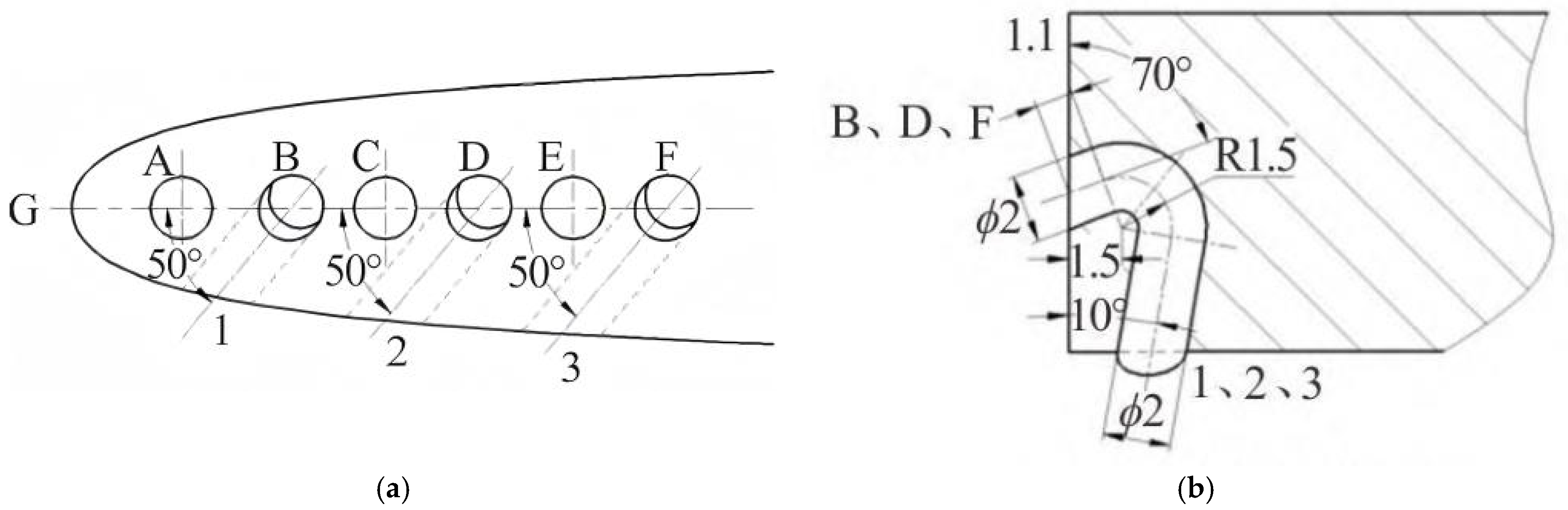
The original NACA0009 hydrofoil had a chord length of 100 mm, a maximum thickness of 9.9 mm, and a spanwise length of 105 mm. For the modified hydrofoil, the hole-pit structures were arranged within the first 20% of the chord length from the leading edge of the hydrofoil tip. Three hemispherical pits and three jet through-holes were alternately distributed in the chordwise direction. The detailed geometric arrangement of the hole-pit structures is shown in Figure 1.

As shown in Figure 1a, the hemispherical pits were located at positions A, C, and E, whereas the jet through-holes were located at positions B, D, and F. Taking the hydrofoil leading−edge point G as the chordwise origin, the center positions A−F were located at x/c = 0.035,0.070, 0.100, 0.130, 0.160, and 0.190, respectively. The diameters of both the hemispherical pits and the jet through−holes were 2 mm. The structural spacing satisfied GA = AB = 3.5 mm and BC = CD = DE = EF = 3 mm. In the tip−surface view shown in Figure 1a, the axes of the jet through-holes were oriented at 50° relative to the chordwise reference direction. The detailed sectional geometry of the jet through-holes is shown in Figure 1b. The principal hydrofoil geometry and operating conditions used in the cavitation-image analysis are summarized in

Table 2. Hydrofoil geometry and operating conditions used in the cavitation−image analysis.

Parameter	Baseline	Case 1	Case 2
Chord length, c (mm)	100	100	100
Maximum thickness (mm)	9.9	9.9	9.9
Spanwise length (mm)	105	105	105
Tip clearance (mm)	3	5	5
Angle of attack (°)	10	10	8
Incoming velocity (m/s)	7.92	7.41	7.94
Experimental role	Baseline analysis	Enlarged tip clearance	Reduced angle of attack at enlarged tip clearance

.

The original hydrofoil and the hydrofoil with hole−pit structures are considered here as two experimental configurations exhibiting different cavitation behaviors. They are not assumed a priori to represent two predefined cavitation states. Instead, the differences in their cavitation images are used to examine whether the proposed image-derived descriptors respond to variations in cavitation behavior.

For the quantitative temporal analysis, 3000 consecutive image samples were used for each analyzed cavitation−area signal. The resulting TLV and TSV time−series signals contained 3000 sampling points over a duration of 30 s, with a temporal interval of 0.01 s between adjacent samples. Accordingly, an effective analysis sampling frequency of 100 Hz was used for the subsequent time−domain, frequency−domain, and time−frequency analyses. The analyzed images had a spatial resolution of 1280 × 1024 pixels. The principal image−sequence parameters used in the present analysis are summarized in

Table 3. Image−sequence parameters used for quantitative cavitation analysis.

Parameter	Value
Image resolution	1280 × 1024 pixels
Number of analyzed samples	3000
Analysis duration	30 s
Temporal interval	0.01 s
Effective analysis sampling frequency	100 Hz
Analyzed regions	TLV, TSV, and six local regions A−F
Analysis type	Offline image post-processing

.

In the present study, 100 Hz denotes the effective sampling frequency used for the image-derived time−series analysis. The nominal camera acquisition frame rate and any original downsampling procedure could not be reliably recovered from the archived experimental metadata; therefore, 100 Hz is reported only as the effective sampling frequency of the analyzed image-derived signals.

2.2. Cavitation Image Preprocessing and Region Extraction

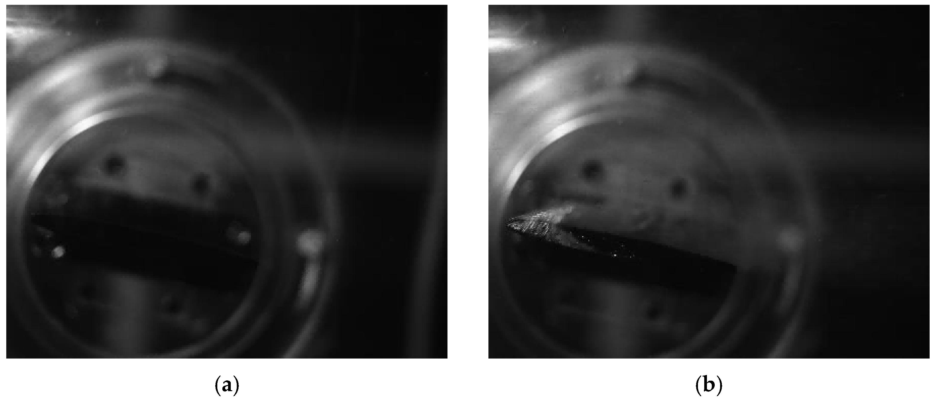
Figure 2 shows the static experimental background and a representative cavitation image before preprocessing. The original images contain stationary background structures, relatively low contrast between the cavitation structures and the surrounding flow field, and locally blurred or discontinuous boundaries. These characteristics complicate the direct extraction of quantitative cavitation information.

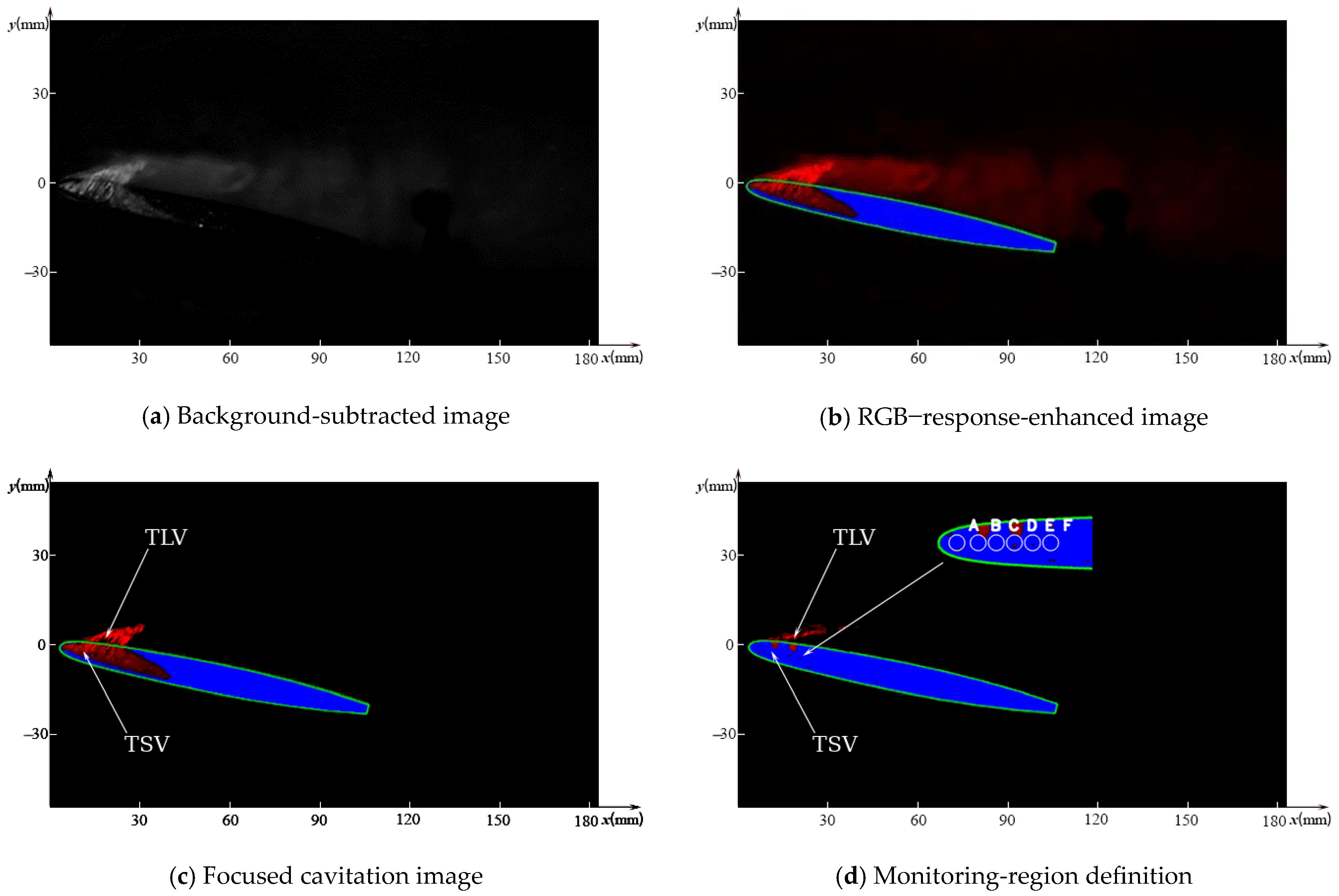
Therefore, a consistent image−processing procedure was applied to all analyzed image sequences before the construction of the image−derived monitoring signals. The procedure consisted of static−background subtraction, RGB−channel−response-based enhancement, Canny edge detection, morphological processing, and threshold-based focusing of the principal tip−leakage cavitation region. The same processing procedure was applied to the two hydrofoil configurations and the three operating conditions to maintain consistency in the subsequent quantitative analysis.

First, static−background subtraction was performed to reduce interference from stationary structures in the experimental images. A reference image representing the static experimental background was subtracted from each cavitation image using a JavaScript batch-processing procedure implemented in ImageJ (version 1.54f). Let I_raw(x,y) denote the original cavitation image and I_bg(x,y) denote the static−background image. The background-subtracted image I_sub(x,y) is expressed as

$$I_{sub}\left(x,y\right)=I_{\mathrm{raw}}\left(x,y\right)-I_{\mathrm{bg}}\left(x,y\right)$$

(1)

After background subtraction, the contrast between the cavitation structures and the surrounding regions remained relatively weak. The RGB channels of the background-subtracted images were therefore separated and reconstructed according to their different intensity responses in the original image−processing procedure. This RGB−response-based reconstruction increased the distinction among the cavitation region, hydrofoil surface, and background and facilitated the subsequent extraction of cavitation boundaries. The purpose of this processing step was to improve feature separability for quantitative cavitation analysis rather than to claim an improvement in the overall perceptual quality of the images.

The enhanced images were subsequently processed using Canny edge detection [49] to identify the principal cavitation boundaries. Because locally fragmented or discontinuous boundaries could remain after edge detection, morphological closing was applied to connect neighboring boundary segments and improve the spatial continuity of the extracted cavitation regions.

Because the present study focuses on cavitation associated with the hydrofoil tip-leakage region, image regions outside the principal focused region were excluded from the subsequent quantitative analysis. During the original image−processing procedure, the red−channel intensity distribution of the RGB−response-enhanced images was examined to distinguish the principal focused tip−leakage cavitation region from lower-intensity background and out-of-focus regions. The principal cavitation region was found to be concentrated mainly at red−channel intensity values above 145. Accordingly, the following fixed criterion was adopted:

R > 145

(2)

Pixels satisfying Equation (2) were retained for the subsequent focused−region analysis, whereas pixels below this threshold were excluded. Importantly, the same threshold was applied to all analyzed image sequences for both hydrofoil configurations and all three operating conditions without case-specific adjustment, thereby maintaining processing consistency among the compared datasets.

The $R>145$ criterion should nevertheless be regarded as a dataset-specific empirical processing setting rather than as a universally validated cavitation−segmentation threshold. Its applicability may depend on illumination conditions, camera settings, background characteristics, and the RGB−response−enhancement procedure. Because the complete archived image−processing dataset does not permit reliable retrospective reprocessing using alternative threshold values, a systematic threshold−sensitivity analysis could not be performed in the present study. Therefore, no claim is made that R = 145 represents an optimal threshold beyond the present experimental image set. Future work should evaluate the sensitivity of the extracted cavitation descriptors to threshold variation and, where possible, compare the segmentation results with manually annotated reference images.

As shown in Figure 3d, the processed images were further organized according to the TLV, TSV, and six local regions A−F for subsequent quantitative cavitation−area analysis. The definitions and use of these monitoring regions are described in Section 2.3.

The principal image−processing procedures and settings are summarized in

Table 4. Image−processing procedure and principal settings used for cavitation−region extraction.

Processing Step	Method or Setting	Purpose
Background removal	Static−background subtraction	Suppress stationary experimental background
Batch processing	JavaScript procedure implemented in ImageJ	Perform consistent frame-by−frame processing
Feature enhancement	RGB−channel−response−based reconstruction	Increase distinction between cavitation and surrounding regions
Boundary extraction	Canny edge detection	Identify principal cavitation boundaries
Morphological processing	Closing operation	Connect locally fragmented boundary segments
Tip−region focusing	Fixed empirical criterion, $R>145$	Retain the principal focused tip−leakage cavitation region
Application scope	Same processing procedure for all analyzed sequences	Maintain consistency among configurations and operating conditions

.

2.3. Monitoring Regions and Cavitation−Area Signal Construction

Following cavitation−region extraction, quantitative analysis was performed using the TLV, TSV, and six local monitoring regions A–F shown in Figure 3d. The TLV and TSV regions represent the two principal cavitating vortex structures in the hydrofoil−tip flow field and were used to characterize their overall temporal evolution. In addition, regions A–F were introduced to describe local spatial variations in cavitation along the hydrofoil−tip region.

The locations of A–F were defined with reference to the chordwise structural positions shown in Figure 1a. Taking the hydrofoil leading−edge point G−as the chordwise origin, the center positions A–F correspond to x/c = 0.035, 0.070, 0.100, 0.130, 0.160, and 0.190, respectively. Positions A, C, and E correspond to the hemispherical−pit locations, whereas B, D, and F correspond to the jet−through-hole locations. The same spatial reference positions were maintained throughout the analyzed image sequences, providing a consistent basis for comparing local cavitation variations between the two hydrofoil configurations and among the different operating conditions.

For each monitoring region, the cavitation area was calculated frame by frame from the extracted cavitation pixels. Let $s\text{\_}i\left(n\right)$ denote the cavitation area associated with monitoring region $i$ in the $n$-th analyzed frame, where $i$ represents the TLV, TSV, or one of the local regions A–F. To reduce the influence of the absolute image scale and facilitate comparison among different image sequences, the extracted cavitation area was nondimensionalized as

$$s_i^{*}={\displaystyle \frac{s_i(n)}{S_h}}$$

(3)

where $s_i^{*}(n)$ is the dimensionless cavitation area, $s_i(n)$ is the extracted cavitation area in the $n$-th frame, and $S_h$ denotes the end−face area of the hydrofoil tip. The same normalization procedure was applied to all analyzed image sequences.

The frame-by-frame dimensionless cavitation areas were subsequently arranged in chronological order to construct continuous image-derived time−series signals,

$$s_i^{*}=\left[s_i^{*}\left(1\right),s_i^{*}\left(2\right),\dots s_i^{*}(N)\right]$$

(4)

where N = 3000 is the number of consecutive samples in each analyzed signal. With an effective analysis sampling frequency of 100 Hz, the temporal interval between adjacent samples was $\Delta t=0.01 \mathrm{s}$, corresponding to a total analysis duration of 30 s. In this manner, the consecutive cavitation images were converted from individual visual frames into temporally connected quantitative signals.

The TLV and TSV area signals were used to characterize the temporal evolution of the principal cavitation structures, whereas the A–F measurements provided local spatial information along the hydrofoil−tip region. These image-derived signals were subsequently characterized from temporal, spatial, frequency−domain, and time−frequency perspectives, as described in Section 2.4.

2.4. Multi-Domain Feature Extraction

The image-derived cavitation−area signals constructed in Section 2.3 were characterized from temporal, spatial, frequency−domain, and time−frequency perspectives. These feature domains were used to describe different aspects of cavitation behavior rather than as independent detection algorithms. The temporal features characterize the overall cavitation level and its variation with time, the local A–F measurements provide spatial information, the frequency−domain features describe the distribution of periodic and broadband fluctuations, and the time−frequency features characterize the temporal evolution of fluctuations at different scales.

For the temporal characterization, the mean dimensionless cavitation area of each monitoring signal was calculated as

$${\overline{s}}_i^{*}={\displaystyle \frac{1}{N}}{\displaystyle \sum _{n=1}^N{s}_i^{*}}(n)$$

(5)

where N = 3000, The mean value was used to represent the overall cavitation level within the corresponding monitoring region, while the complete time−series signal retained information on temporal fluctuations. For the local regions A–F, the mean dimensionless areas at the six chordwise locations were compared to characterize the spatial distribution of cavitation along the hydrofoil−tip region.

To characterize the frequency content of the cavitation−area fluctuations, Fast Fourier Transform (FFT) analysis was applied to the image-derived time−series signals. Before the FFT calculation, the mean value of each signal was removed to reduce the dominance of the zero-frequency component:

$${\tilde{s}}_i^{*}(n)=s_i^{*}(n)-{\overline{s}}_i^{*}$$

(6)

The discrete Fourier transform of the mean-removed signal was then calculated as

$$X_i(k)={\displaystyle \sum _{n=1}^N{s}_i^{*}}(n)\exp \left[-j{\displaystyle \frac{2\pi k\left(n-1\right)}{N}}\right],\hspace{1em}k=0,1,\dots ,N-1$$

(7)

For the present signals, N = 3000 and the effective analysis sampling frequency was $f_s=100$ Hz. Accordingly, the single-sided spectra were evaluated over the range of 0–50 Hz, corresponding to the Nyquist frequency of 50 Hz. It should be noted that the 50 Hz upper frequency limit is determined by the effective analysis sampling frequency of 100 Hz. Because the nominal camera acquisition frequency and the original downsampling procedure could not be reliably reconstructed from the archived experimental metadata, the 0–50 Hz range should be interpreted as the frequency scale of the analyzed image-derived signals rather than as a fully reconstructed representation of the original camera-frequency content. Accordingly, the spectral characteristics are used primarily for comparative analysis between signals processed using the same procedure. The nominal frequency spacing associated with the 3000-sample analysis window was

$$\Delta f={\displaystyle \frac{f_s}{N}}={\displaystyle \frac{100}{3000}}\approx 0.0333 \mathrm{Hz}$$

(8)

The spectral amplitude and its distribution over the analyzed frequency range were used to characterize periodic components, harmonic behavior, and broadband fluctuations of the cavitation−area signals. To provide quantitative spectral descriptors for the cross-condition evaluation, the dominant non-zero frequency and the corresponding maximum spectral amplitude were additionally extracted from the TLV and TSV signals under Cases 1 and 2. The dominant frequency, $f_{\mathrm{d}\mathrm{o}\mathrm{m}}$, was defined as the frequency corresponding to the maximum amplitude of the mean-removed single-sided spectrum, excluding the zero-frequency component. For the quantitative amplitude descriptor, the single-sided spectral amplitude was calculated as $A(f_k)=2\left|X(k)\right|/N$ for the positive non-Nyquist frequency components, and the corresponding maximum value was denoted as $A_{\mathrm{m}\mathrm{a}\mathrm{x}}$. These descriptors were used for descriptive and comparative characterization of the spectral responses rather than as classification thresholds. Because the cavitation−area signals also contain non-stationary fluctuations, Discrete Wavelet Transform (DWT) was used to provide a multi-scale time−frequency representation. Each signal was decomposed into seven detail components, D₁–D₇, and a seventh-level approximation component, A₇:

$$s_i^{*}(t)=A_7(t)+{\displaystyle \sum _{j=1}^7{D}_j}(t)$$

(9)

At the effective sampling frequency of 100 Hz, the dyadic decomposition corresponded approximately to the frequency ranges 25–50 Hz for D₁, 12.5–25 Hz for D₂, 6.25–12.5 Hz for D₃, 3.13–6.25 Hz for D₄, 1.56–3.13 Hz for D₅, 0.78–1.56 Hz for D₆, 0.39–0.78 Hz for D₇, and 0–0.39 Hz for A₇. Thus, the detail components describe fluctuations at progressively lower frequency scales, whereas A₇ retains the low-frequency variation trend.

The same temporal, spatial, FFT, and DWT procedures were applied to both hydrofoil configurations under the baseline condition and the two changed operating conditions summarized in Table 2. The purpose of the multi-domain analysis was to determine whether changes in cavitation behavior were reflected consistently in complementary descriptors of cavitation level, spatial distribution, spectral fluctuation, and multi-scale temporal variation.

2.5. Cross-Condition Evaluation and Data−Representation Assessment

To examine whether the extracted image-derived features remained responsive when the operating condition changed, the same image−processing, area−normalization, and multi-domain feature−extraction procedures were applied to the baseline condition, Case 1, and Case 2. No case-specific modification of the processing workflow was introduced. The baseline condition was used for the primary comparison between the two hydrofoil configurations, whereas Case 1 and Case 2 were used for cross-condition evaluation under changed operating conditions.

For each 30 s cavitation−area signal, the mean value was used to characterize the overall cavitation level, while the complete time−series signal was retained to describe its temporal variation. Because the available dataset does not contain independently repeated experimental runs for all operating conditions, repeatability-based uncertainty estimates and statistical significance tests were not performed. The 3000 consecutive samples in each signal represent temporal observations within a single analyzed sequence and are therefore not treated as independent experimental repetitions.

For comparisons between the original hydrofoil and the hydrofoil with hole−pit structures, the relative reduction in the mean dimensionless cavitation area was calculated as

$${\eta }_i={\displaystyle \frac{\overline{s_{i,\mathrm{ori}}^{*}}-\overline{s_{i,\mathrm{hp}}^{*}}}{\overline{s_{i,\mathrm{ori}}^{*}}}}\times 100\%$$

(10)

where $\overline{s_{i,ori}^{*}}$ and $\overline{s_{i,hp}^{*}}$ denote the mean dimensionless cavitation areas of the original hydrofoil and the hydrofoil with hole−pit structures, respectively. The same comparison procedure was applied to the TLV, TSV, and local monitoring regions under the three operating conditions. These comparisons are used to evaluate the responsiveness of the extracted features to changes in hydrofoil configuration and operating condition rather than to demonstrate predictive classification performance beyond the analyzed dataset.

In addition to feature responsiveness, the reduction in data dimensionality obtained by converting the image sequences into image-derived monitoring signals was estimated. Each analyzed frame contained 1280 × 1024 = 1,310,720 pixels, whereas the monitoring representation consisted of eight scalar area values per time step, corresponding to the TLV, TSV, and six local regions A−F. For a sequence of N−frames, the dimensionality− reduction factor can therefore be expressed as

$$R_{\dim }={\displaystyle \frac{1280\times 1024\times N}{8N}}=\mathrm{163,840}$$

(11)

Thus, in terms of the number of image pixels relative to the extracted monitoring quantities, the area−signal representation reduces each image frame from 1,310,720 spatial pixels to eight area descriptors before subsequent temporal, spectral, and time−frequency characterization. This comparison is intended to quantify the compactness of the proposed feature representation rather than to represent an experimentally measured communication−compression ratio. Actual transmission load would additionally depend on image encoding, numerical precision, communication protocol, and network implementation.

The present study therefore evaluates the proposed approach at the visual sensing and feature−representation level. No underwater communication link, edge−computing platform, or automatic cavitation classifier was implemented. The extracted compact descriptors are instead intended to provide candidate monitoring information that could be integrated into future IoUT−based cavitation−monitoring and autonomous−detection systems.

3. Results

The results are first presented under the baseline operating condition to examine the temporal and spatial responses of the image-derived cavitation features. Frequency−domain and time−frequency characteristics are then analyzed, followed by an evaluation under the two changed operating conditions.

3.1. Temporal and Spatial Characteristics of Cavitation-Area Signals

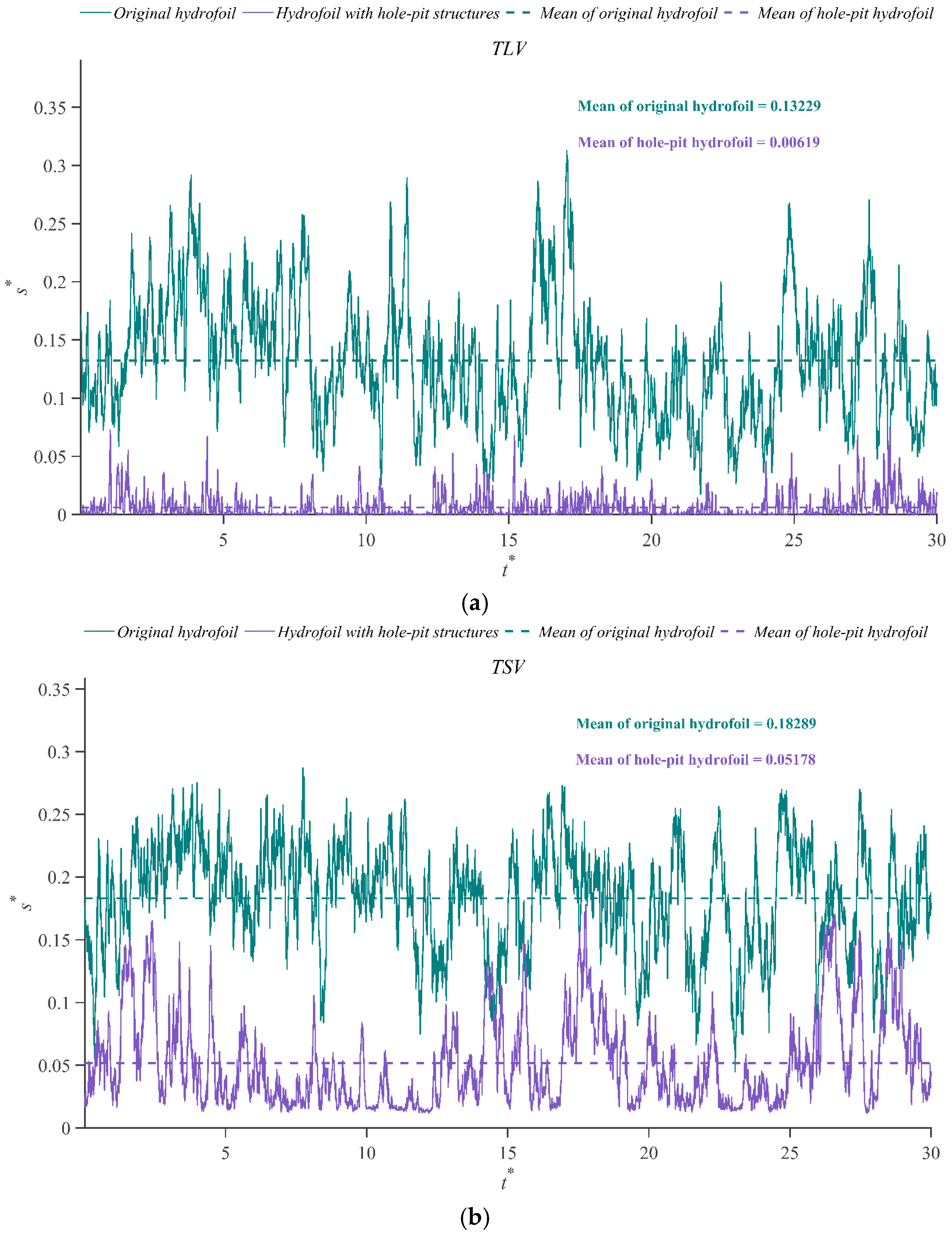
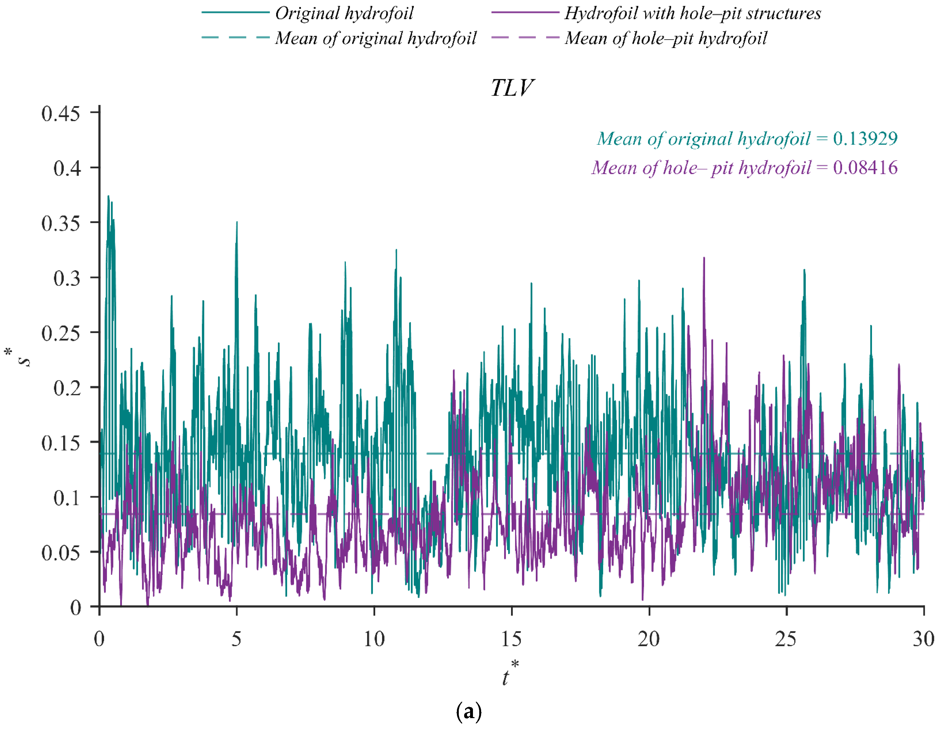
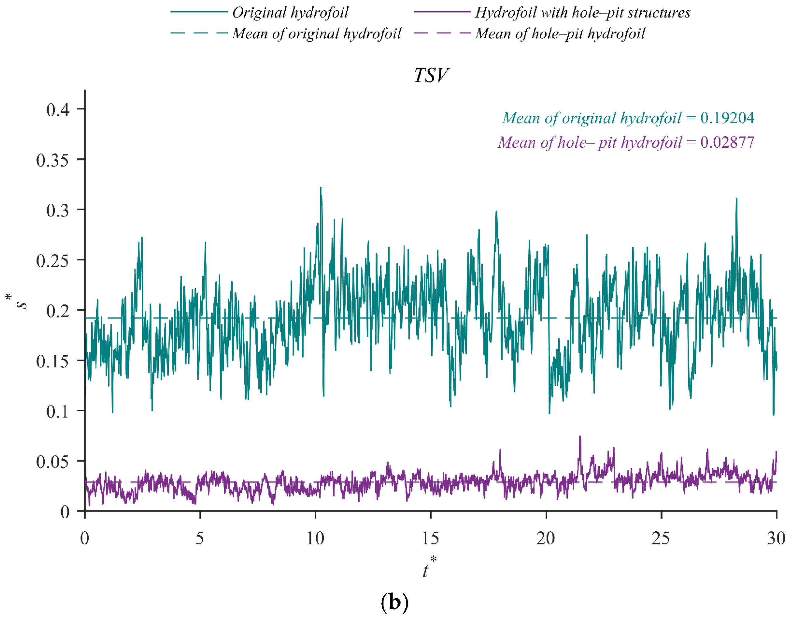
Figure 4 presents the temporal variations in the dimensionless TLV and TSV cavitation−area signals for the original hydrofoil and the hydrofoil with hole−pit structures under the baseline condition. Both signals exhibit continuous temporal fluctuations over the 30 s analysis period, indicating that the consecutive cavitation images retain information on the unsteady evolution of the cavitating structures rather than only their time-averaged extent.

The mean dimensionless cavitation areas provide a compact measure of the overall cavitation level within the two principal monitoring regions. Compared with the original hydrofoil, the mean TLV and TSV cavitation areas of the hydrofoil with hole−pit structures were approximately 40.0% and 85.0% lower, respectively. These differences demonstrate that the image-derived area signals respond clearly to changes in hydrofoil configuration. The response magnitude was greater in the TSV region than in the TLV region under the baseline condition, indicating that the two monitoring regions provide different but complementary information on cavitation behavior.

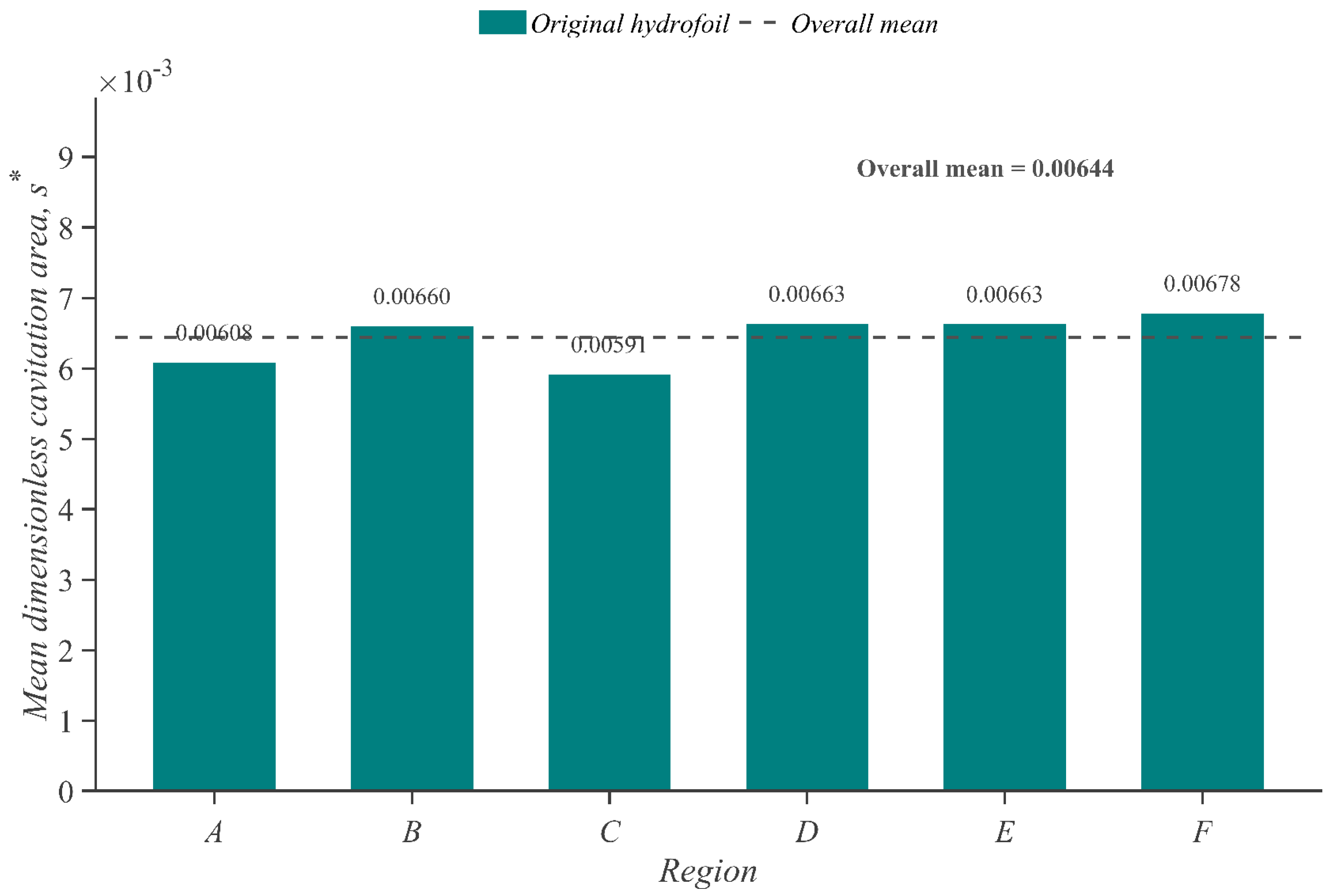
In addition to the global TLV and TSV signals, the local regions A–F were examined to characterize spatial variations along the hydrofoil−tip region. Figure 5 presents the mean dimensionless cavitation areas at the six local positions for the original hydrofoil. The mean values were relatively similar among the six regions, indicating a comparatively uniform spatial distribution of the local cavitation−area measure under the baseline condition.

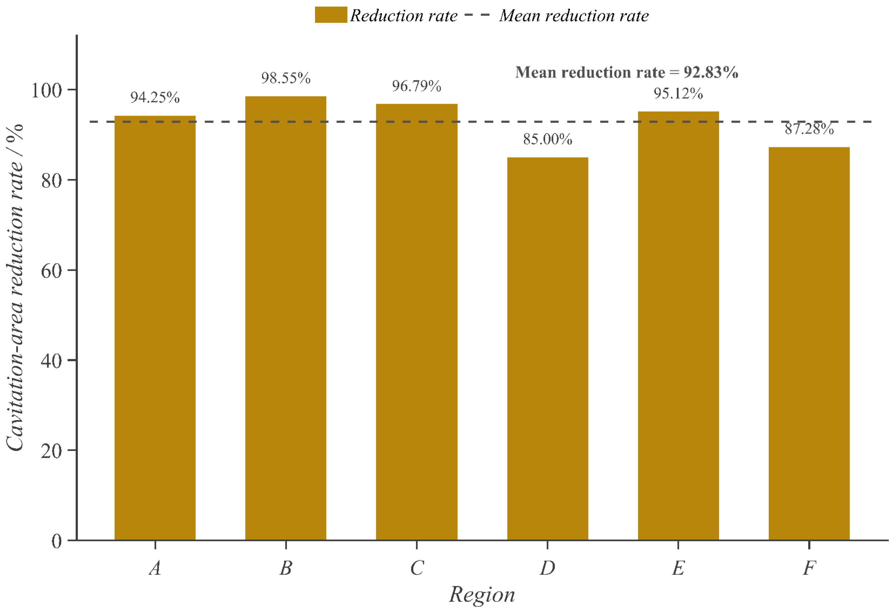
Figure 6 further compares the relative reductions in mean cavitation area between the two hydrofoil configurations at regions A–F. Larger reductions were observed at regions A, B, C, and E, whereas regions D and F exhibited comparatively smaller reductions. This spatial variation shows that the response of a local cavitation−area descriptor depends on its monitored position. Consequently, the six local regions provide complementary spatial information that cannot be represented by the global TLV and TSV areas alone.

Overall, the baseline results show that the image-derived cavitation−area representation provides two levels of monitoring information. The TLV and TSV signals describe the temporal evolution and overall level of the principal cavitation structures, whereas the A–F measurements describe their local spatial variation. These temporal and spatial characteristics are subsequently complemented by frequency−domain and time−frequency analysis.

3.2. Frequency−Domain Characteristics

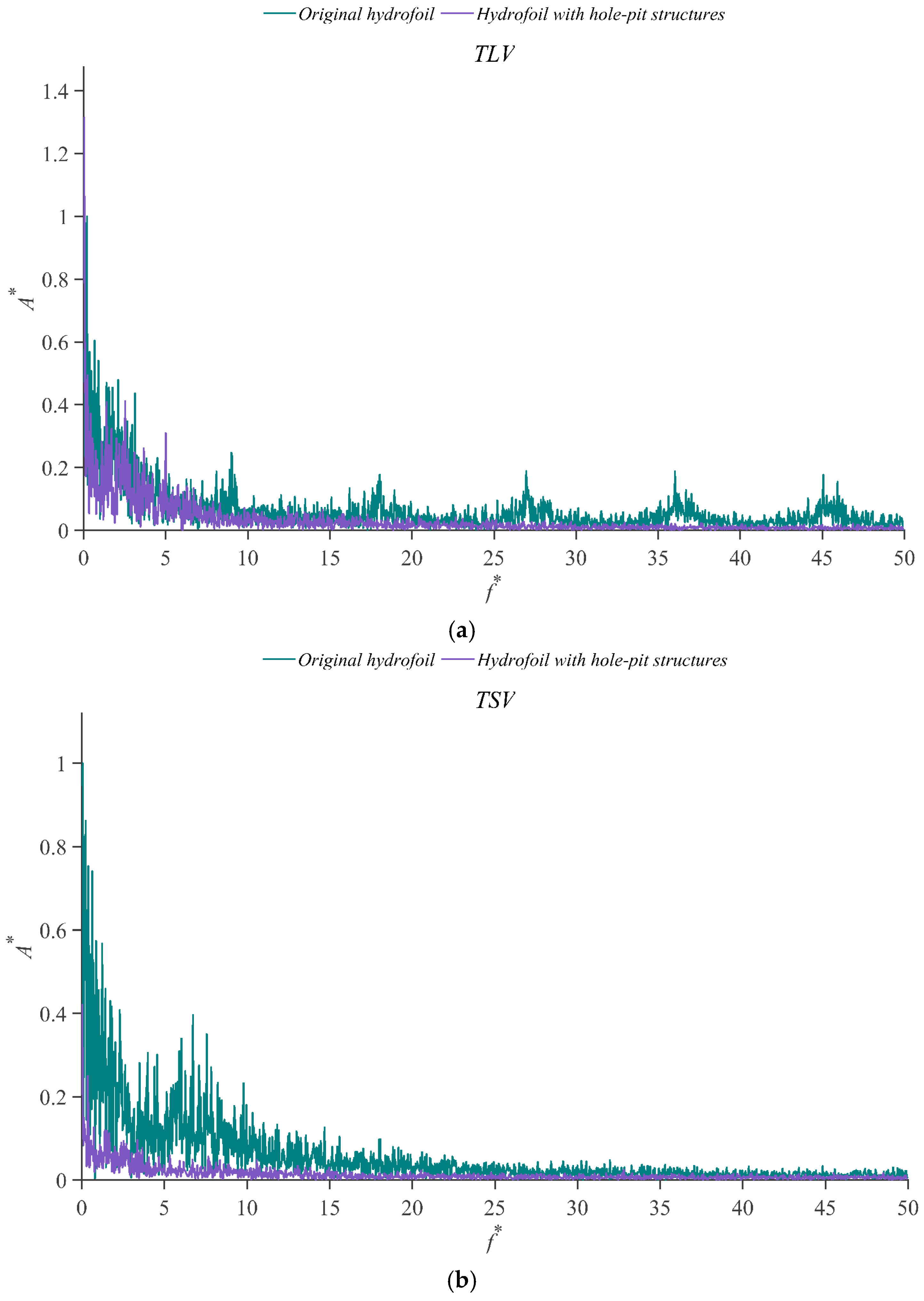
Figure 7 presents the frequency−domain characteristics of the TLV and TSV cavitation−area signals for the original hydrofoil and the hydrofoil with hole−pit structures under the baseline condition. The spectra were obtained using the FFT procedure described in Section 2.4, with the mean value removed before transformation so that the spectral distributions primarily represent the fluctuating components of the cavitation−area signals.

For the TLV signal of the original hydrofoil, several relatively distinct spectral peaks were observed, indicating the presence of periodic or harmonic components in the cavitation−area fluctuations. In contrast, the TLV spectrum of the hydrofoil with hole−pit structures exhibited lower spectral amplitudes over a substantial part of the analyzed frequency range, with the spectral amplitudes more strongly concentrated in the low-frequency region. The difference was particularly evident in the higher-frequency components. These results indicate that the frequency−domain representation captures differences in the unsteady TLV cavitation behavior that are not fully described by the mean cavitation area alone.

For the TSV signal, the spectral distribution differed from that of the TLV. Distinct harmonic behavior was less evident, while differences in spectral amplitude between the two hydrofoil configurations remained observable over a broad portion of the analyzed frequency range. This result is consistent with the different temporal responses of the TLV and TSV area signals and further indicates that the two monitoring regions contain complementary dynamic information.

Overall, the frequency−domain results show that changes in hydrofoil configuration are reflected not only in the mean cavitation−area level but also in the distribution of fluctuation amplitudes across frequency. Therefore, the FFT-derived spectral characteristics provide an additional description of cavitation dynamics that complements the temporal and spatial area features.

3.3. Time−Frequency Characteristics

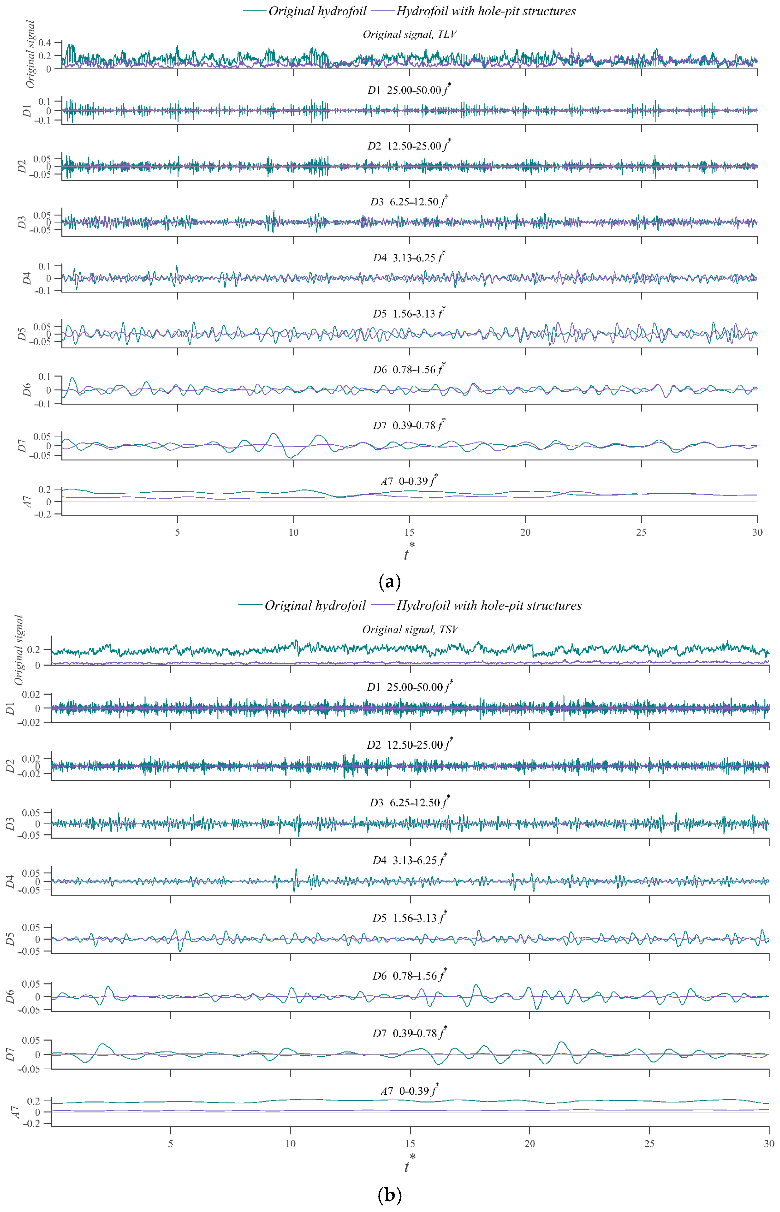
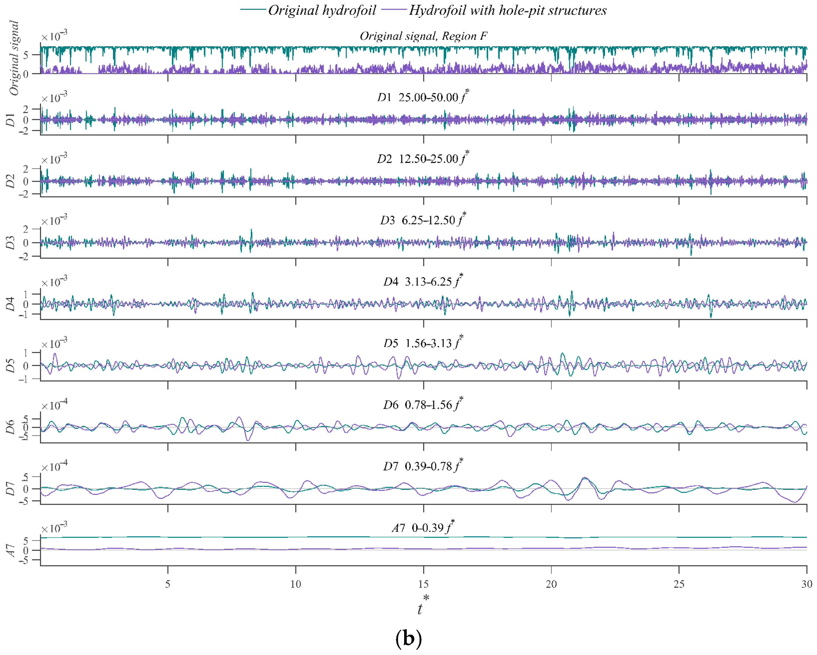
Figure 8 presents the DWT results of the TLV and TSV cavitation−area signals for the two hydrofoil configurations under the baseline condition. The decomposition separates the original area signals into detail components D₁–D₇ and the low−frequency approximation component A₇,thereby allowing for the temporal evolution of fluctuations at different frequency scales to be examined.

For the TLV signal of the original hydrofoil, similar fluctuation patterns were observed in several higher-frequency detail components, which is consistent with the harmonic characteristics identified by the FFT analysis in Figure 7a. In comparison, the hydrofoil with hole-pit structures exhibited lower fluctuation amplitudes in several higher-frequency components, whereas the differences in the lower-frequency components were less pronounced. This result shows that the DWT representation retains the frequency-dependent differences observed in the FFT spectra while additionally revealing how these fluctuations evolve with time.

For the TSV signal, the fluctuation amplitudes were more strongly represented in the lower-frequency components, and the temporal patterns differed among the wavelet scales. Differences between the two hydrofoil configurations remained observable in multiple detail components as well as in the low-frequency variation trend. Compared with the TLV, the TSV therefore exhibited a different multi-scale temporal response, further demonstrating that the two cavitation regions contain complementary dynamic information.

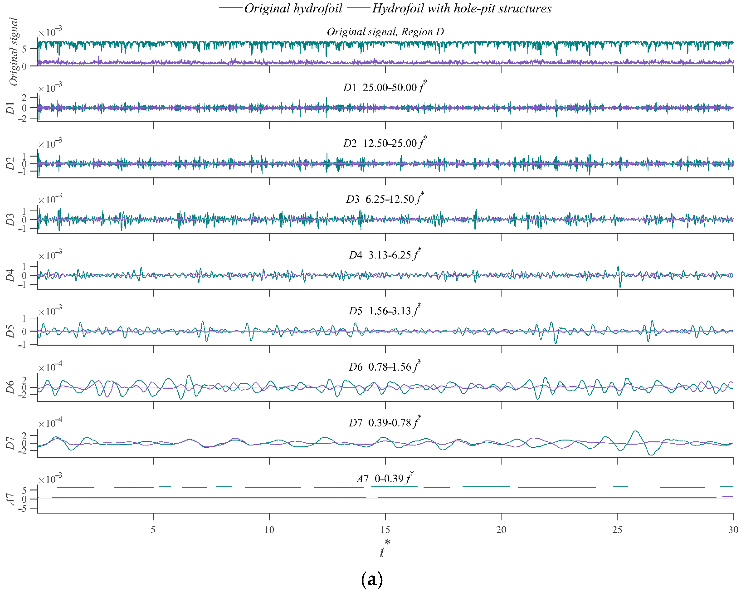
To further examine whether the time–frequency representation can reveal local differences that are less evident from the mean cavitation−area values, regions D and F were selected for additional analysis. These two regions exhibited comparatively smaller relative reductions in mean cavitation area in the spatial analysis of Section 3.1. Their DWT results are shown in Figure 9.

In region D, differences between the two hydrofoil configurations were more apparent in several higher-frequency detail components, whereas some lower-frequency components exhibited relatively similar amplitudes during portions of the analyzed period. In region F, differences were likewise observed in part of the higher-frequency range, while relatively pronounced low-frequency fluctuations occurred during several time intervals.

The results from regions D and F are particularly relevant because their relative reductions in mean cavitation area were smaller than those of several other local regions. The additional differences revealed by the wavelet components indicate that a limited response in a time-averaged area feature does not necessarily imply similar temporal dynamics. Accordingly, the DWT-derived characteristics complement the mean−area and FFT features by retaining information on both fluctuation scale and temporal localization.

Overall, the baseline results demonstrate complementary roles for the different feature domains. The mean cavitation area describes the overall cavitation level, the A–F measurements characterize local spatial variation, FFT describes the distribution of fluctuation amplitudes over frequency, and DWT further resolves the temporal evolution of fluctuations at different scales.

3.4. Cross-Condition Evaluation of the Extracted Features

To examine whether the image-derived features remained responsive under changed operating conditions, the same processing and multi-domain feature−extraction procedure was applied to Case 1 and Case 2. As summarized in Table 2, Case 1 represents an operating condition with an enlarged tip clearance, whereas Case 2 combines the enlarged tip clearance with a reduced angle of attack. Because the incoming velocity also varies among the three cases, these additional cases are treated as cross-condition evaluations rather than as controlled single-parameter sensitivity tests.

This evaluation therefore does not aim to establish universal cavitation thresholds or classification performance. Instead, it examines whether the temporal, spatial, frequency domain, and time–frequency descriptors identified under the baseline condition continue to exhibit observable differences between the two hydrofoil configurations when the operating condition changes.

3.4.1. Temporal and Spatial Responses

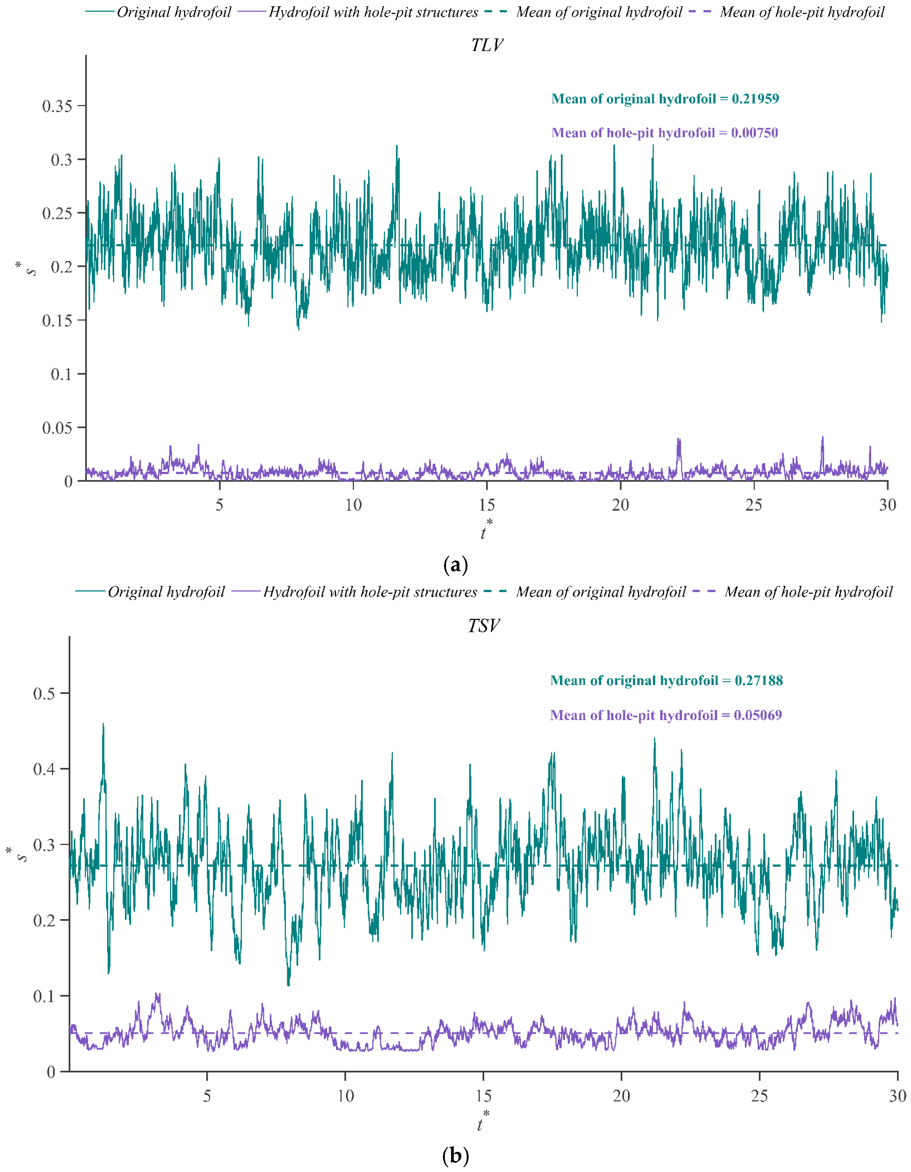
Figure 10 presents the TLV and TSV cavitation−area signals under Case 1. Clear differences between the two hydrofoil configurations remained observable throughout the analyzed period. For the TLV, the mean dimensionless cavitation area decreased from 0.219591 for the original hydrofoil to 0.007503 for the hydrofoil with hole-pit structures, corresponding to a relative reduction of 96.58%. For the TSV, the corresponding mean value decreased from 0.271885 to 0.050687, representing a reduction of 81.36%.

Compared with the baseline results, the relative responses of TLV and TSV changed considerably. Under the baseline condition, the relative reduction was larger for TSV than for TLV, whereas under Case 1 the TLV exhibited the larger relative reduction. This change indicates that the relative response of an individual monitoring region is dependent on the operating condition and that neither TLV nor TSV should be treated as a universally dominant indicator.

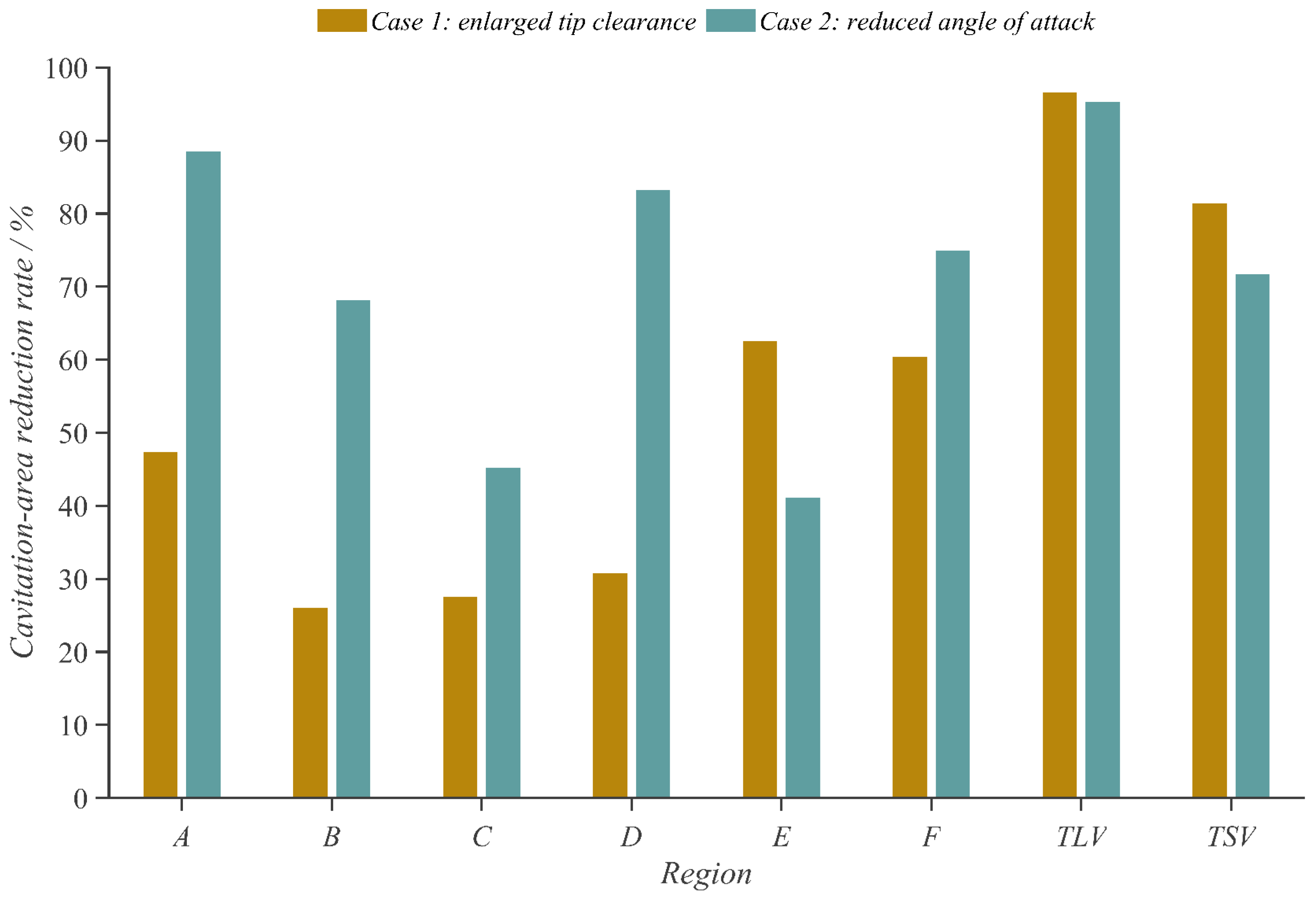
The local A–F measurements also retained spatial differences under Case 1. The relative reductions in regions A–F were 47.37%, 25.99%, 27.51%, 30.75%, 62.50%, and 60.34%, respectively. Thus, the magnitude of the local response was not uniform along the chordwise monitoring positions, with regions E and F exhibiting larger relative reductions than regions B-D under this operating condition.

Figure 11 presents the corresponding temporal signals under Case 2. The mean dimensionless TLV cavitation area decreased from 0.132286 to 0.006186, corresponding to a relative reduction of 95.32%, whereas the mean TSV cavitation area decreased from 0.182888 to 0.051783, corresponding to a reduction of 71.69%. Clear differences between the two hydrofoil configurations therefore remained observable in both principal monitoring regions.

For the local regions A–F under Case 2, the corresponding reduction rates were 88.54%, 68.17%, 45.16%, 83.20%, 41.09%, and 74.96%, respectively. The spatial distribution of these relative reductions differed markedly from that obtained under Case 1. For example, regions A and D showed substantially larger relative responses in Case 2, whereas region E showed a smaller response than in Case 1. This result further indicates that the information provided by a single local monitoring position may change with the operating condition.

Figure 12 summarizes the relative reductions in mean cavitation area for regions A–F, TLV, and TSV under the two additional operating conditions.

Differences between the two hydrofoil configurations were observed for all monitored regions under both cases, but their magnitudes varied substantially with monitoring location and operating condition. The results therefore support the use of multiple image-derived area descriptors rather than reliance on a single global or local area feature. The reported percentages are specific to the operating conditions examined here and are not intended as universal reduction rates for other tip clearances, angles of attack, or inflow conditions.

3.4.2. Frequency-Domain Responses

The frequency-domain characteristics under the two changed operating conditions were subsequently examined using the same FFT procedure as that applied to the baseline signals. Because the signal mean was removed before transformation as described in Section 2.4, the spectra primarily represent the fluctuating components of the image-derived cavitation-area signals.

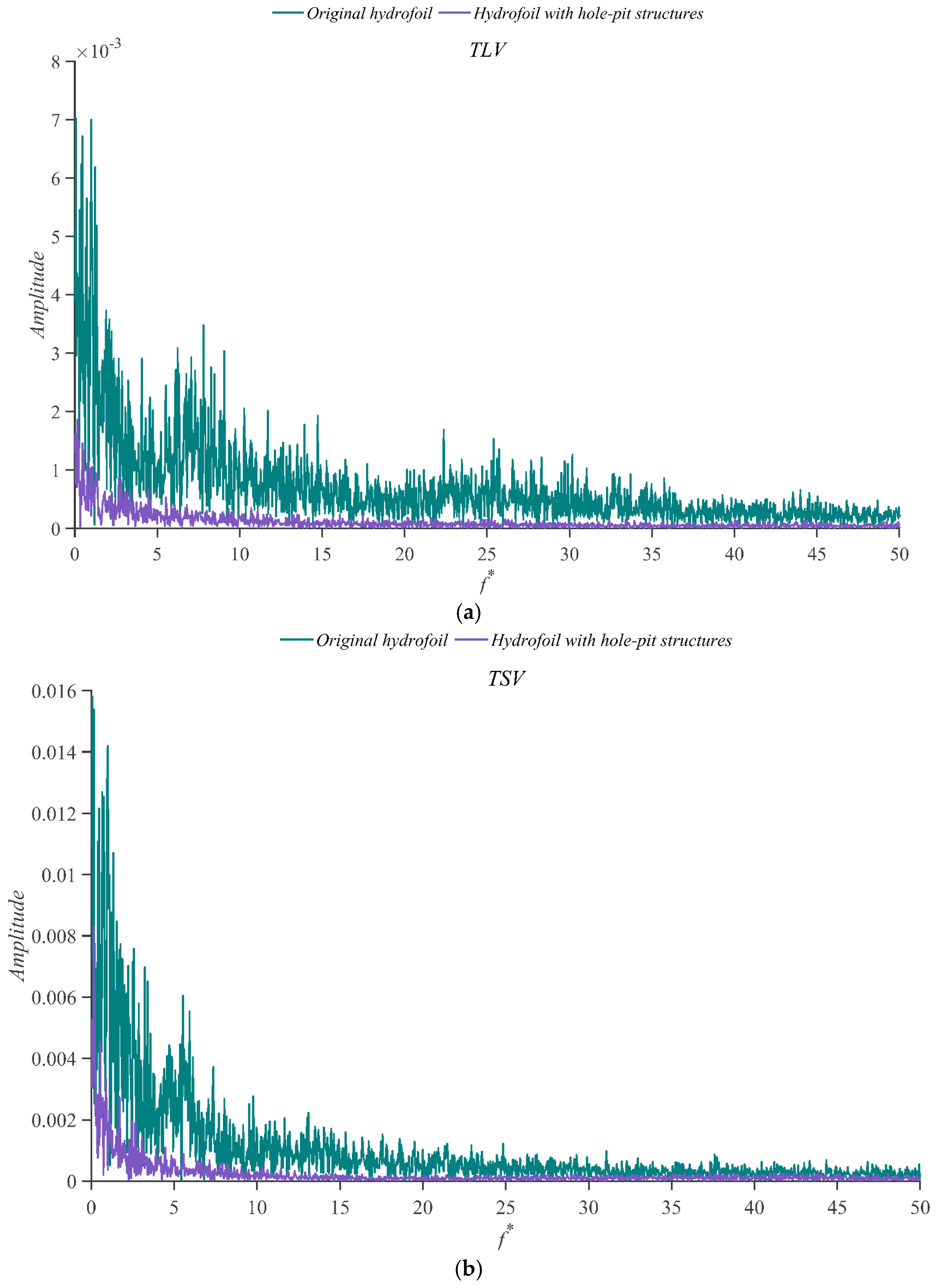
Figure 13 presents the TLV and TSV spectra under Case 1. For the original hydrofoil, the spectral amplitudes were concentrated mainly in the lower-frequency portion of the analyzed range. The hydrofoil with hole-pit structures exhibited lower amplitudes over a substantial part of the spectrum, while the overall low-frequency-dominated distribution remained evident. Differences between the two hydrofoil configurations were observed for both TLV and TSV.

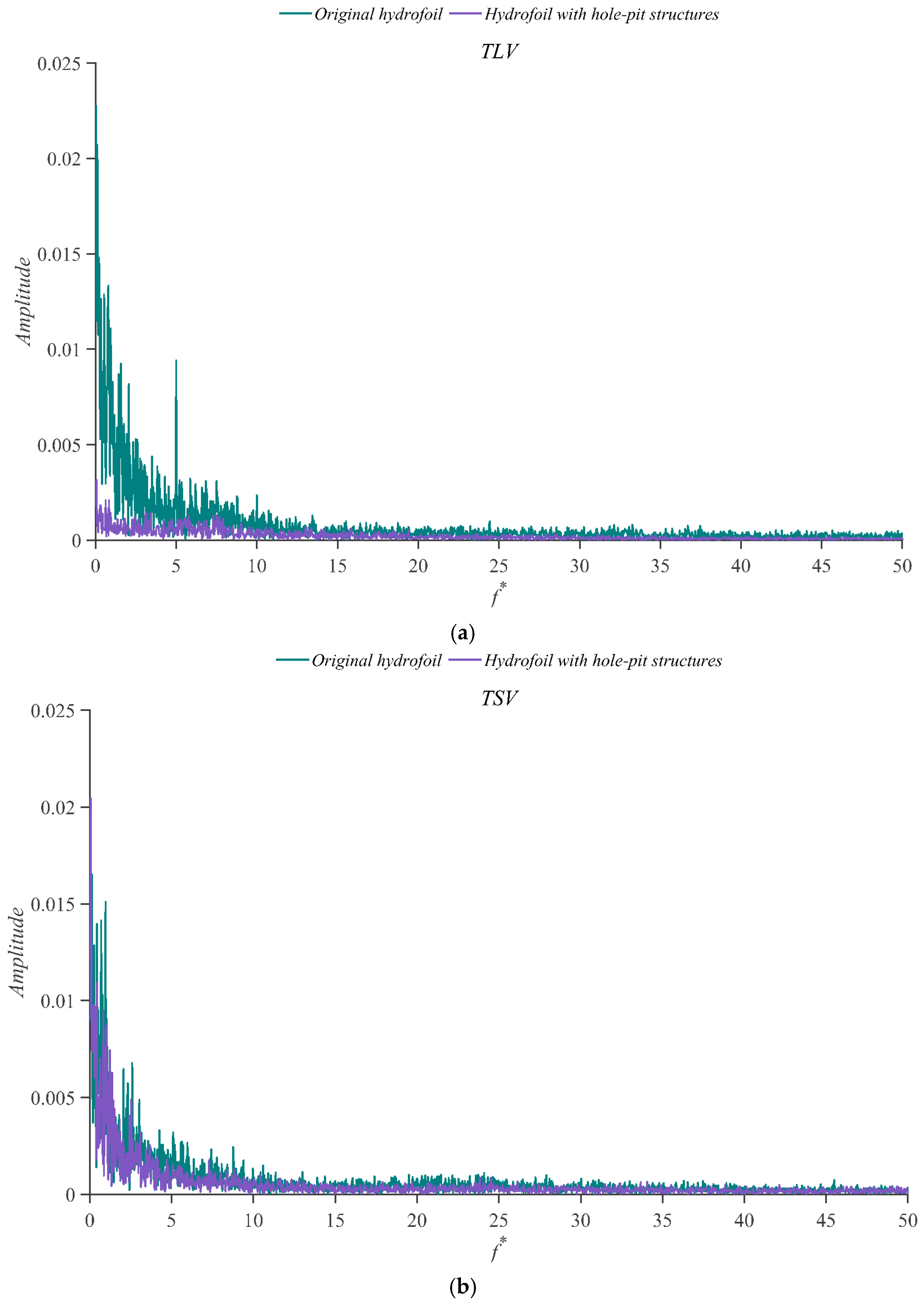
Figure 14 shows the corresponding spectra under Case 2. Similar to Case 1, the fluctuation amplitudes were predominantly concentrated in the lower-frequency range, while differences between the two hydrofoil configurations remained observable across much of the analyzed spectrum. The relative spectral responses of TLV and TSV were not identical, consistent with the different temporal-area responses described in Section 3.4.1.

The quantitative FFT descriptors in

Table 5. Quantitative FFT descriptors of the TLV and TSV cavitation-area signals under Cases 1 and 2.

Condition	Region	fdom, Original (Hz)	fdom, Hole-Pit (Hz)	Amax, Original	Amax, Hole-Pit
Case 1	TLV	0.067	0.167	0.007030	0.001862
Case 1	TSV	0.067	0.167	0.015802	0.008314
Case 2	TLV	0.033	0.067	0.022813	0.003155
Case 2	TSV	0.133	0.067	0.016519	0.020452

provide numerical characterization of the spectral differences observed in Figure 13 and Figure 14. Under Case 1, the dominant frequencies of both the TLV and TSV signals shifted from 0.067 Hz for the original hydrofoil to 0.167 Hz for the hydrofoil with hole-pit structures, while the corresponding maximum spectral amplitudes decreased from 0.007030 to 0.001862 for the TLV and from 0.015802 to 0.008314 for the TSV. Under Case 2, the dominant TLV frequency changed from 0.033 to 0.067 Hz, accompanied by a decrease in Amax from 0.022813 to 0.003155. For the TSV, the dominant frequency changed from 0.133 to 0.067 Hz, whereas Amax increased from 0.016519 to 0.020452. These results indicate that the configuration-dependent spectral response is not characterized by a uniform decrease in spectral amplitude and varies with both the monitored cavitation region and operating condition.

Taken together, the graphical spectra and the quantitative FFT descriptors indicate that the low-frequency-dominated spectral character of the cavitation-area fluctuations is retained across the operating conditions considered, while the dominant frequency and maximum spectral amplitude exhibit configuration- and region-dependent variations. Thus, the FFT-derived representation provides dynamic information that is complementary to the mean-area descriptors and remains informative when the operating condition changes.

3.4.3. Time–Frequency Responses

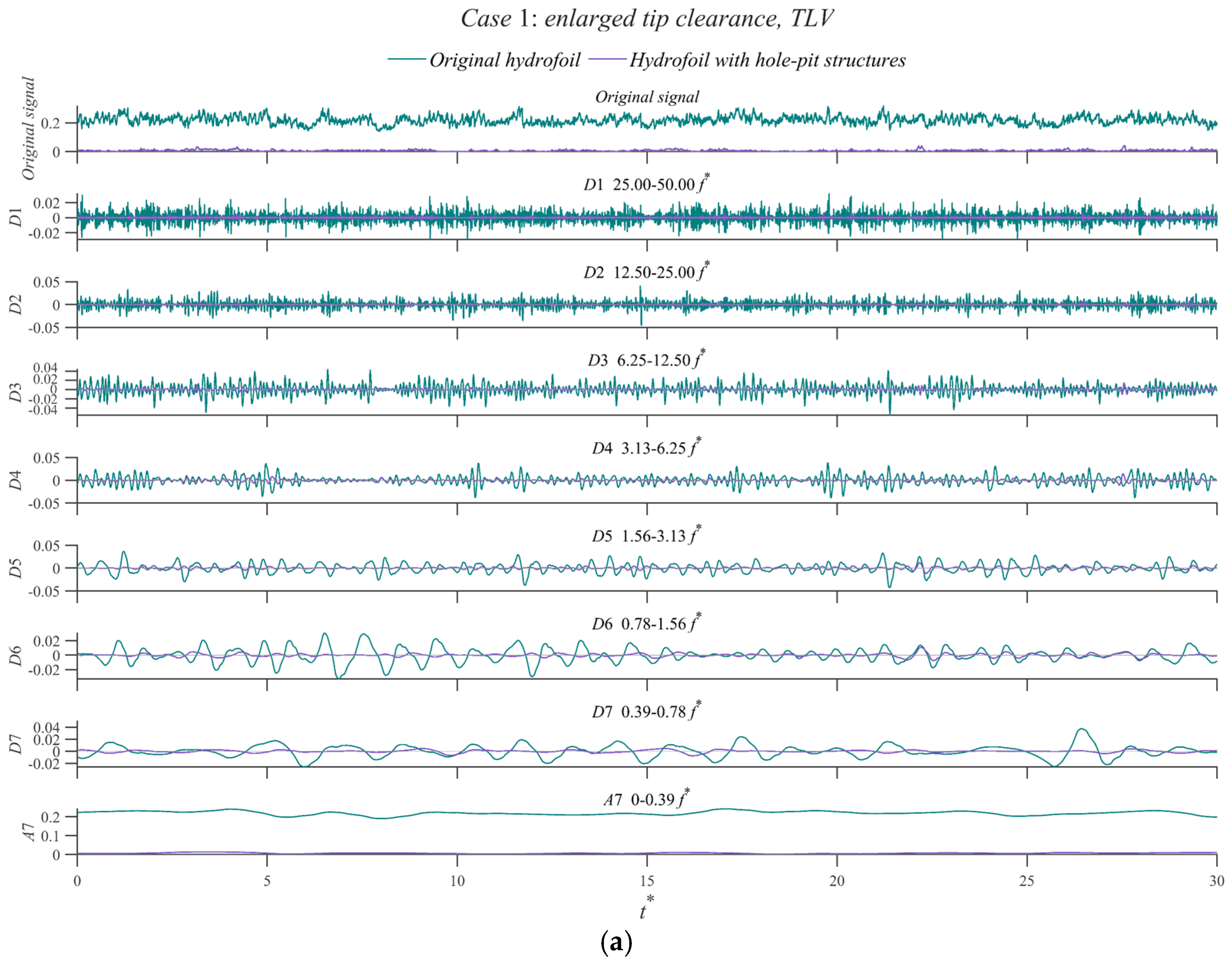
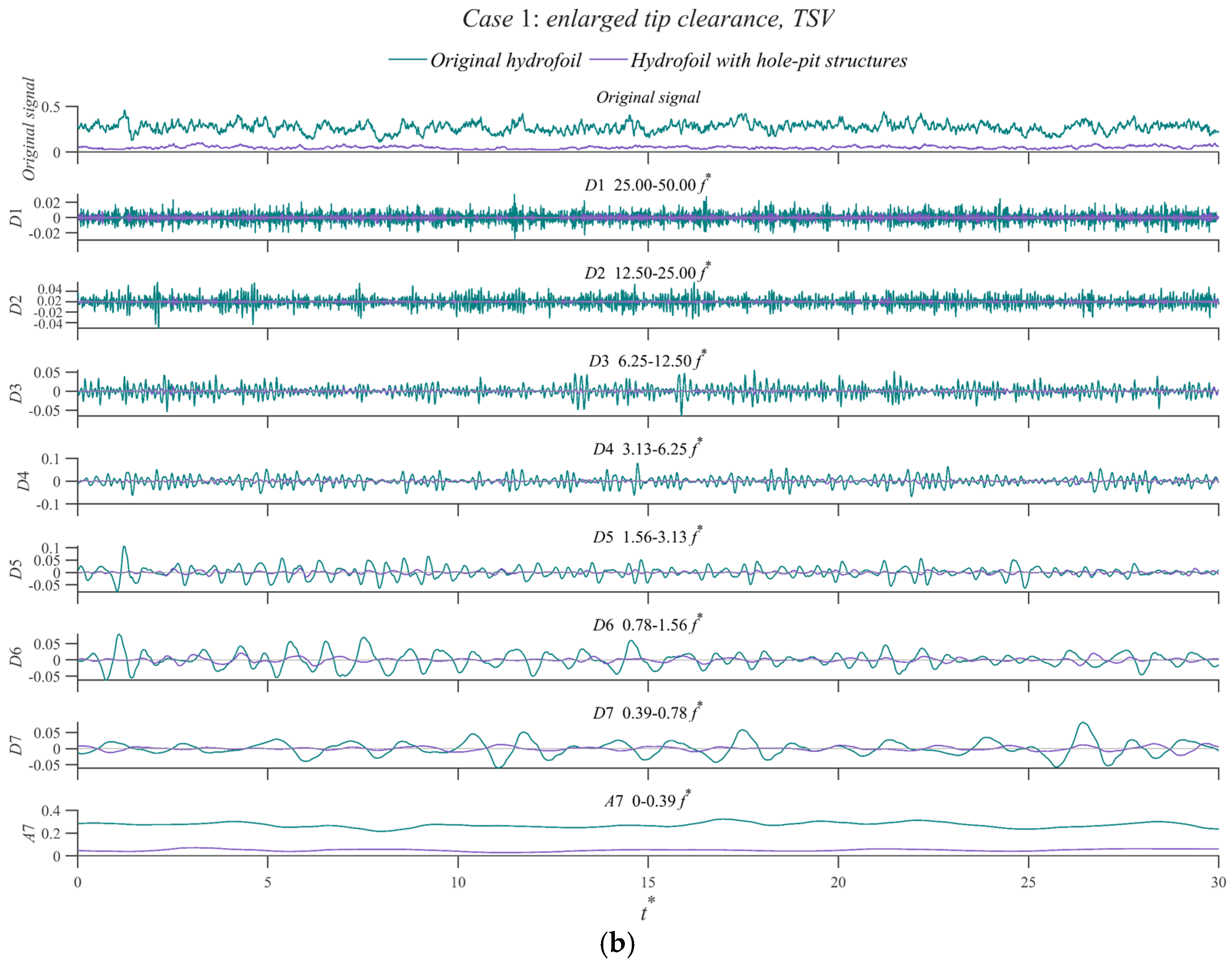
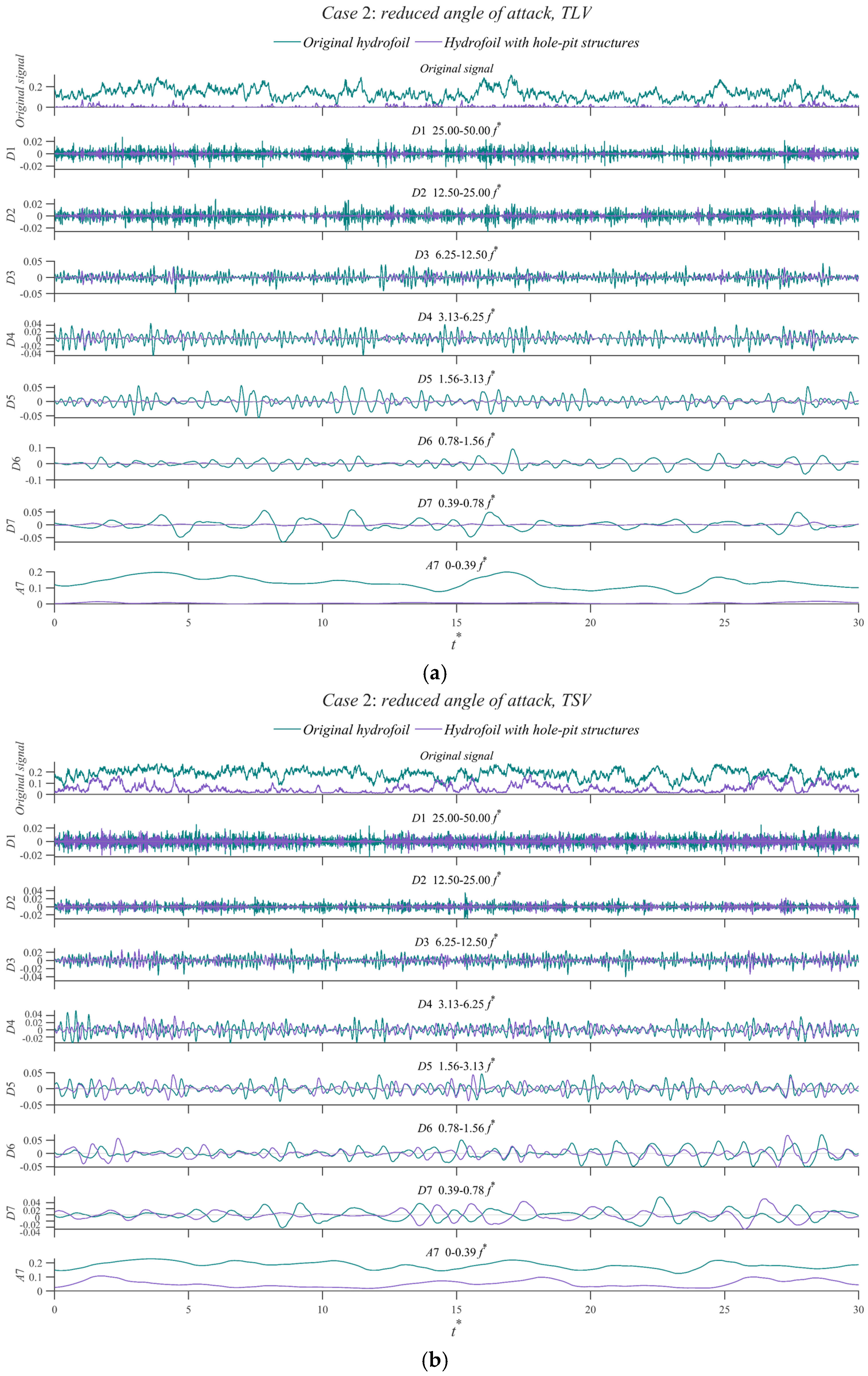
The DWT results were further examined to determine whether the multi-scale temporal differences observed under the baseline condition remained visible under the two changed operating conditions. Figure 15 and Figure 16 present the decomposition results for Cases 1 and 2, respectively.

Figure 15 shows the DWT components of the TLV and TSV signals under Case 1. Differences between the two hydrofoil configurations were observed in several detail components, particularly within the higher-frequency scales. At the same time, the low-frequency approximation component A7 retained the slowly varying trend of the corresponding cavitation-area signals.

The differences in the detail components show that the two hydrofoil configurations exhibit different local fluctuation patterns even after the signals are separated into individual frequency scales. These observations are consistent with the spectral−amplitude differences identified in Figure 13, while the DWT representation additionally preserves the temporal locations of the fluctuations.

Figure 16 presents the DWT results under Case 2. Differences between the two hydrofoil configurations remained visible in multiple detail components of both the TLV and TSV signals. The low-frequency approximation component was retained for both configurations, whereas several higher-frequency detail components exhibited differences in fluctuation amplitude and temporal variation.

The results from Cases 1 and 2 therefore show that the multi-scale characteristics identified under the baseline condition are not restricted to a single operating condition. In particular, configuration-dependent differences remain observable in several wavelet detail components, whereas A₇ retains the slower temporal variation of the cavitation−area signals. The DWT representation consequently complements the time−domain and FFT results by providing temporally localized information at multiple fluctuation scales.

Overall, the cross-condition evaluation shows that the relative magnitude of individual features varies with operating condition and monitoring location, but differences between the two hydrofoil configurations remain observable in temporal, spatial, frequency−domain, and time−frequency representations. The results should therefore be interpreted as evidence of cross-condition responsiveness within the present experimental dataset, rather than as proof of universal discrimination capability. This multi-domain representation provides the basis for the subsequent discussion of feature complementarity and its potential use in image-based cavitation monitoring.

4. Discussion

4.1. Complementarity of Multi-Domain Cavitation Features

The results demonstrate that no single image-derived feature provides a complete description of the cavitation behavior observed in the present experiments. Instead, the temporal, spatial, frequency−domain, and time−frequency representations describe different aspects of the cavitation process. The mean cavitation area provides a compact measure of the overall cavitation level, whereas the complete area time series retains information on temporal fluctuations. The local regions A–F further introduce spatial resolution along the hydrofoil−tip region, while FFT and DWT characterize dynamic information that is not directly represented by time-averaged area measurements.

The distinction from previous monitoring approaches is primarily associated with the type and continuity of information retained for analysis. Conventional underwater or IoUT-oriented monitoring based on pressure, vibration, acoustic, or other scalar signals provides compact measurements of specific physical quantities but generally contains limited direct information on the spatial morphology of cavitation. Underwater image-processing studies preserve rich visual information, but their outputs often emphasize image enhancement, segmentation, or target visibility rather than temporally connected monitoring descriptors. Cavitation−image studies provide physically meaningful quantities such as cavity area, length, morphology, and boundary position, but many analyses rely primarily on representative frames or time-averaged characteristics. Conversely, conventional signal−processing approaches can describe temporal, spectral, and time−frequency behavior but do not inherently preserve spatially localized visual information. The present study does not replace these approaches; rather, it connects continuous cavitation imagery with temporally connected area signals and complementary spatial, spectral, and multi-scale temporal descriptors within a single monitoring-oriented representation. This integrated representation constitutes the principal distinction of the present workflow.

The complementary roles of the TLV and TSV signals are particularly evident from their different responses under the examined operating conditions. Under the baseline condition, the relative reduction between the two hydrofoil configurations was larger for the TSV than for the TLV, whereas under Case 1 and Case 2 the TLV exhibited the larger relative reduction. This variation indicates that the usefulness of an individual cavitation-area descriptor depends on the operating condition. Consequently, TLV and TSV measurements should be regarded as complementary monitoring variables rather than interchangeable indicators or universally dominant features.

A similar conclusion can be drawn from the local A–F measurements. The spatial distribution of the relative cavitation−area reductions changed substantially between the baseline condition, Case 1, and Case 2. For example, regions D and F showed comparatively smaller reductions under the baseline condition, whereas the relative responses of the six local regions changed considerably under the additional operating conditions. These observations suggest that a feature extracted from a single spatial location may not remain equally informative when the operating condition changes. Spatially distributed measurements therefore provide information that would be lost if cavitation were represented only by a single global area value.

The frequency−domain and time−frequency results provide a further level of complementary information. FFT analysis revealed differences in the distribution of fluctuation amplitudes across frequency even when the mean cavitation area alone could not describe the dynamic characteristics of the signals. DWT additionally retained the temporal localization of fluctuations at different scales. This distinction is particularly relevant for regions D and F, where the relative reductions in mean cavitation area were comparatively small, but differences remained visible in several wavelet components. Thus, a relatively small change in a time−averaged area descriptor does not necessarily imply similar unsteady cavitation behavior.

The cross-condition results further reinforce the need for a multi-domain representation. Although the relative magnitude of individual features varied with monitoring position and operating condition, configuration-dependent differences remained observable in temporal, spatial, frequency−domain, and time−frequency representations. The principal value of the proposed approach therefore lies not in any individual image−processing or signal−processing algorithm, but in organizing continuous cavitation observations into a set of complementary quantitative descriptors. Such a representation is more suitable for monitoring-oriented analysis than reliance on a single averaged quantity and provides a broader feature basis for future cavitation−detection methods.

4.2. Implications for IoUT-Oriented Cavitation Monitoring

The relevance of the proposed approach to IoUT-oriented monitoring lies primarily in the representation of visually acquired cavitation information rather than in the implementation of a complete underwater communication system. Continuous cavitation images contain detailed spatial and temporal information, but their direct transmission would require substantially larger data volumes than conventional scalar sensing signals. The present workflow addresses this issue at the feature−representation stage by converting each processed image into a small set of physically interpretable monitoring quantities associated with the TLV, TSV, and six local regions A–F. This positioning is consistent with the scope defined in the present study, which focuses on visual sensing and feature representation rather than on the development of an underwater communication architecture.

For the analyzed images, each frame contains $1280 \times 1024 = \mathrm{1,310,720}$ spatial pixels, whereas the area-based monitoring representation contains eight descriptors at each time step. As defined in Section 2.5, this corresponds to a pixel−count-to-descriptor count reduction factor of 163,840. The value should not be interpreted as a measured communication−compression ratio, because the actual data volume transmitted through an IoUT link would additionally depend on image encoding, bit depth, numerical precision of the extracted features, packet structure, communication protocol, and network configuration. Instead, the reduction factor quantifies the compactness of the proposed information representation before any communication−layer implementation.

The compact representation is potentially useful for underwater monitoring because it preserves several forms of cavitation information without requiring the complete image sequence to be used as the primary monitoring output. The TLV and TSV area signals retain the overall temporal evolution of the principal cavitating structures, the A–F descriptors provide spatially distributed information, and the FFT- and DWT-derived characteristics further describe spectral and multi-scale temporal variations. Thus, the proposed representation differs from a simple image−compression strategy: rather than attempting to reconstruct the original visual data, it extracts monitoring-oriented quantities that are directly related to the observed cavitation behavior.

This approach may complement conventional underwater monitoring based on pressure, vibration, acoustic, or other scalar sensor measurements. Such sensors are efficient for measuring specific physical quantities, whereas image-derived descriptors can retain direct information about the spatial distribution and temporal evolution of cavitation. The two forms of sensing should therefore be regarded as potentially complementary rather than mutually exclusive. In a future IoUT implementation, the extracted visual descriptors could be combined with other sensing variables to provide a more informative representation of propulsion−system operating conditions.

The present results also indicate a possible pathway toward future edge-assisted cavitation monitoring. Image acquisition and preprocessing could be performed near the sensing side, followed by the extraction of compact cavitation descriptors for subsequent storage, transmission, or higher-level analysis. However, this study did not implement an underwater communication link, edge−computing platform, communication protocol, or real-time transmission experiment. Therefore, no claim is made regarding achievable bandwidth savings, communication latency, energy consumption, or real-time computational performance in an actual IoUT network. These aspects require dedicated hardware and network-level validation in future work.

Overall, the proposed method can be interpreted as a visual sensing and feature−extraction component that could be incorporated into a broader IoUT monitoring framework. Its main contribution at this stage is the conversion of data-intensive cavitation image sequences into compact, physically interpretable, multi-domain descriptors. Such descriptors may reduce reliance on the transmission of complete image sequences and provide suitable inputs for future cavitation−monitoring and autonomous−detection systems, while the practical communication and real-time implementation remain to be established experimentally.

4.3. Limitations and Future Development

Several limitations should be considered when interpreting the present results. First, the analysis was based on two hydrofoil configurations and three experimental operating conditions, and independently repeated experimental runs were not available for all cases. Importantly, the 3000 consecutive samples used to construct each cavitation−area signal represent temporal observations within a single analyzed image sequence rather than 3000 independent experimental replicates. They therefore cannot be treated as independent samples for estimating experimental repeatability or statistical significance. Accordingly, the reported percentage differences and cross-condition comparisons should be interpreted primarily as descriptive and comparative results within the present dataset rather than as inferential evidence applicable to a broader operating envelope. Future experiments should include independent repeated acquisitions under identical operating conditions and a wider range of tip clearances, angles of attack, inflow velocities, and cavitation conditions to enable uncertainty quantification and more rigorous statistical evaluation.

Second, the temporal sampling information used for the frequency−domain and time−frequency analyses constitutes an additional limitation. The nominal camera acquisition frequency and the original downsampling procedure could not be reliably recovered from the archived experimental metadata. Consequently, although the analyzed image-derived signals have an effective sampling frequency of 100 Hz and a corresponding Nyquist limit of 50 Hz, the influence of the original acquisition and downsampling procedures on the retained frequency content cannot be retrospectively quantified. In particular, the absolute physical interpretation of higher−frequency spectral components should therefore be treated with caution. The FFT and DWT results in the present study are primarily used for comparative characterization among signals processed using the same analysis procedure rather than for reconstructing the complete original frequency content of the cavitation dynamics.

Third, the cavitation−region extraction procedure contains dataset-dependent image-processing settings. In particular, the R > 145 criterion was determined empirically from the red−channel intensity distribution of the available experimental images and was applied consistently to all analyzed image sequences. However, a systematic threshold−sensitivity analysis or independent manual−segmentation validation was not available for the present dataset. The threshold should therefore be regarded as a dataset-specific processing criterion rather than as a universally optimal segmentation threshold under different illumination conditions, camera settings, background characteristics, or imaging environments. In addition, the local monitoring regions A–F were defined according to fixed structural reference positions for the present hydrofoil configuration. Future work should evaluate threshold sensitivity and agreement with manually annotated reference images and should investigate adaptive or data-driven segmentation methods together with standardized spatial registration of monitoring regions under varying imaging conditions and hydrofoil geometries.

Fourth, the present multi-domain analysis is intended to characterize cavitation behavior rather than to provide a completed cavitation classifier. No classification decision threshold, feature−selection procedure, supervised or unsupervised classification model, or predictive−performance metric such as accuracy, sensitivity, specificity, precision, recall, or F1 score was evaluated in the present study. Accordingly, the temporal, spatial, frequency−domain, and time−frequency characteristics reported here should be interpreted as monitoring descriptors for descriptive and comparative analysis rather than as evidence of demonstrated automatic cavitation detection. Future work should evaluate the separability and predictive value of these descriptors using independent experimental datasets before incorporating them into cavitation−detection models. Future work should also include a formal ablation study comparing area-only, FFT-only, DWT-only, and combined multi-domain feature sets within a defined detection or classification framework.

Fifth, the present study was performed through offline image processing and did not implement an underwater communication link, edge−computing device, or real-time IoUT monitoring platform. The dimensionality−reduction analysis therefore quantifies the compactness of the image-derived representation rather than actual communication bandwidth, latency, or energy savings. Future work should integrate the proposed feature−extraction workflow with edge-side processing hardware and underwater communication systems, and experimentally evaluate computational cost, transmission load, latency, and performance stability under realistic underwater imaging and networking conditions. Such developments would provide the necessary transition from the present monitoring-oriented feature representation toward practical IoUT-based cavitation monitoring and autonomous detection.

5. Conclusions

This study developed an image-based multi-domain feature−extraction approach for hydrofoil tip leakage flow cavitation monitoring. Consecutive cavitation images were processed to construct dimensionless cavitation−area signals for the TLV, TSV, and six local regions A–F. Temporal and spatial characterization was then combined with FFT and DWT analyses to obtain complementary information on the overall cavitation level, regional distribution, spectral fluctuations, and multi-scale temporal variations.

Under the baseline operating condition, the mean TLV and TSV cavitation areas of the hydrofoil with hole−pit structures were approximately 40.0% and 85.0% lower than those of the original hydrofoil, respectively. The local A–F measurements further showed that the response magnitude depended on the monitored position. Under the two changed operating conditions, differences between the two hydrofoil configurations remained observable in the TLV, TSV, and local cavitation−area descriptors, although their relative magnitudes varied with operating condition and monitoring location. These results indicate that reliance on a single global or local area feature may be insufficient for characterizing changes in cavitation behavior.

The frequency−domain and time−frequency analyses provided additional dynamic information beyond the mean cavitation−area features. For Cases 1 and 2, quantitative FFT analysis showed that the dominant non-zero frequencies of the TLV and TSV signals ranged from 0.033 to 0.167 Hz, while the corresponding maximum spectral amplitudes exhibited configuration- and region-dependent variations. In particular, the maximum spectral amplitude decreased for the TLV under both changed operating conditions and for the TSV under Case 1, whereas an increase was observed for the TSV under Case 2. DWT further retained the temporal localization of fluctuations at different scales and revealed dynamic differences even in local regions where the mean cavitation−area response was comparatively small. The combined results therefore support the use of temporal, spatial, frequency−domain, and time−frequency descriptors as complementary monitoring features rather than as isolated indicators.

From an IoUT-oriented perspective, the proposed approach converts data-intensive cavitation image sequences into a compact set of physically interpretable image-derived descriptors. The present study addresses the visual sensing and feature−representation stage and does not claim implementation of a complete underwater communication network or autonomous cavitation classifier. The extracted descriptors instead provide candidate monitoring information for future integration with edge-side processing, underwater communication, and autonomous cavitation−detection systems. Further work should extend the operating range, include independent repeated experiments, improve adaptive cavitation−region extraction, extend quantitative spectral and wavelet characterization to broader datasets, evaluate feature separability through formal ablation and predictive studies, and assess the proposed representation in a practical IoUT monitoring platform.