1. Introduction
The rapid expansion of cyber infrastructure, driven by the proliferation of mobile and smart devices, has resulted in unprecedented global connectivity, with billions of individuals now integrated into the Internet ecosystem [
1]. The Internet of Things (IoT) refers to the devices that automatically connect to the Internet for data transmission and reception. With billions of connected devices in homes and hospitals, the market is expected to grow to over
$2.4 trillion annually by 2027 [
2]. According to Statista, currently, there are 19.8 billion connected devices, and it predicts there will be 40.6 billion by 2034 [
3]. The devices with weak authentication, lack of encryption, and built-in security mechanisms are vulnerable and prime targets for threats like malware attacks [
4].
IoT devices like Internet cameras, routers, and smart TVs are mostly attacked by IoT malware, which is malicious software created by malicious authors to control these devices. IoT malware is counted as a severe threat because of stealing users’ private information, building botnets to launch attacks on other devices, and breaking the whole network infrastructure. Additionally, Zscaler reports that IoT malware attacks are growing quickly, increasing by 400% by 2023 and 45% in 2024, mainly because many IoT devices are easy to hack, with 66% of these attacks targeting routers [
5,
6,
7]. Commonly, IoT malware is categorized as viruses, worms, and botnets that exploit vulnerable devices by scanning the Internet, gaining access, and infecting them with malicious binary [
8,
9,
10]. Mirai, a renowned IoT malware, appeared in 2016 and became an architecture for inventing new variants like Okiru, Satori, etc., since its source code was published on the Internet [
11]. Estimates suggest that Mirai and its variants have infected nearly 2,500,000 IoT devices worldwide [
12]. A recent report discovered that the leading malware families hitting IoT devices are Mirai (36.3%) and Gafgyt (21.2%) [
7]. Based on the statistics, IoT malware is a major threat to IoT devices due to a lack of efficient anti-malware to safeguard these devices. There is an urgent need to design and propose an accurate, fast, and lightweight IoT malware analysis and detection system.
The major analysis methods are static, dynamic, and hybrid for feature extraction to train ML algorithms for detecting IoT malware. Static is a lighter, faster, and safer method because it extracts features directly from the binary file without running it. Examples are byte sequences, opcodes, strings, header information, and control flow graph (CFG) [
13,
14,
15]. However, the dynamic method is slower, riskier, and heavier because feature extraction from files requires execution within a controlled and isolated environment via monitoring and recording their behavior [
16,
17]. Instances of the dynamic method could be API trace calls, network traffic, and so on. Using a combination of static and dynamic is known as the hybrid method, which has a higher computational overhead than the aforementioned methods [
18].
To propose accurate and swift detection, machine-learning (ML) models need to train on only minimal discriminative features. To achieve this, the feature selection (FS) phase is an essential requirement before training ML algorithms because FS improves their performance by eliminating redundant and noisy features while retaining the ideal features. Therefore, the trained models can precisely distinguish between malicious and non-malicious behaviors. Typically, the FS methods are categorized as filter, wrapper, and embedded. Filter approaches rank features using statistical measurements, requiring less calculation time. Examples encompass information gain (IG) and variance threshold. Wrapper approaches like recursive feature elimination depend on classifier outcomes to identify the optimal feature set, which is more precise due to iterative learning processes and cross-validation. Finally, embedded methods employ ensemble and hybrid learning techniques during model training, which provide superior performance and are less computational than wrapper methods. Instances include Decision Trees (DT), Random Forests (RF), and Light-Gradient-Boosting-Machine (LGBM) [
19].
Numerous researchers have proposed IoT malware detection systems. However, significant gaps persist in this domain, and existing solutions are inadequate due to a lack of public datasets, a reliable FS approach, neglect of its critical role, high dimensionality and class imbalance issues, a lack of rapid detection, dependence on resource-intensive tools, and not being designed for actual operation and implementation on IoT devices.
To address the aforementioned gaps, two novel FS approaches are proposed as an essential solution for enhancing IoT malware detection. The development of a reliable FS approach in this domain depends critically on the chosen method and its ability to accurately identify optimal features. An appropriate FS strategy not only mitigates the dimensionality problem and enhances detection accuracy but also substantially reduces training and inference times, thereby making the model feasible for deployment on resource-constrained IoT devices. In this study, FS approaches were designed, proposed, and implemented by integrating filter, wrapper, and embedded methods to select minimal yet highly discriminative features, effectively resolving the challenges of high dimensionality that typically lead to prolonged training and prediction times, as well as excessive resource consumption conditions inherently misaligned with the constrained nature of IoT devices. The first proposed FS approach is called Intelligent Hybrid Feature Selector 1 (IHFS1), which combines filter-embedded methods utilizing variance threshold (VTH) and the LGBM algorithm. However, the second approach, Intelligent Hybrid Feature Selector 2 (IHFS2), integrates filter-wrapper methods employing VTH and recursive feature elimination with cross-validation (RFE-CV) that uses LGBM as an estimator. To implement the proposed FS approaches, a feature vector was needed. For this purpose, we proposed a fully automated and free-disassembler static analysis pipeline to extract the operation code (opcode) via disassembling the machine code of both IoT malware and benign samples.
Key objectives of this research are to:
Create a self-benign dataset by collecting benign Executable and Linkable Format (ELF) files from widely used Advanced RISC Machine (ARM) IoT operating systems and combining them with public malware samples from the most prevalent families (Mirai, Gafgyt, and Tsunami). This ensures that the dataset reflects the dominant architecture and threat landscape of current IoT environments;
Propose an efficient static analysis pipeline without utilizing existing disassembler tools to extract an informative and accurate static feature, namely opcodes, from the entire dataset;
Propose two novel FS approaches by hybridizing filter, wrapper, and embedded methods to solve the high-dimensionality issue, select the least discriminative feature set, reduce the computational overhead with inference time, and enhance the models’ performance;
Address the imbalance issue that is mostly seen in the cybersecurity era, typically in the IoT malware field;
Evaluate the efficiency and effectiveness of the selected feature sets by training and assessing the performance of various supervised ML classifiers, including tree-based, linear-based, and probabilistic models, in terms of performance metrics and inference time. This evaluation aims to identify an accurate, fast, and lightweight ML detector that is feasible for future deployment on IoT devices to detect IoT malware in near real-time, which is essential for defending IoT devices against threat hazards;
Validate the computational effectiveness and the system’s generalization ability by testing trained models on unseen data and measuring their prediction times, making it practical for deployment in IoT devices.
Core contributions of this research are as follows:
Proposed and validated two novel hybrid FS approaches, IHFS1 and IHFS2, as effective dimensionality reduction techniques for IoT malware detection. The approaches achieved a substantial reduction in dataset dimensionality by efficiently condensing the original feature space, thereby decreasing training and inference times while preserving the predictive performance of ML classifiers. The improvements in computational efficiency were further validated through statistical significance testing (t-test), confirming that the observed gains were not due to chance;
Prepared a distinct IoT malware dataset designated as ARMIoTDS-25 by integrating the ARM samples referenced in [
20] with a self-collected ARM-benign dataset;
Proposed and validated a highly effective static analysis pipeline for IoT malware detection, incorporating a novel, fully Python-based disassembling mechanism that eliminates reliance on heavyweight external tools such as Radare2. To the best of the current knowledge, this is the first study to perform static analysis without incurring traditional disassembler overhead, thereby achieving substantial computational advantages and confirming its suitability for deployment in resource-constrained IoT environments;
Handled the class imbalance issue between IoT malware and benign samples effectively by proposing and configuring eight balanced ML models;
Demonstrated that numerous high-performing classifiers, particularly RF, DT, LGBM, Support Vector Machine (SVM), Gaussian Naïve Bayes (GNB), and Logistic Regression (LR), can attain optimum detection accuracy using the chosen feature sets, validating their superiority and confirming that these features are not specific to a single classifier. This finding is crucial and facilitated the construction of a computationally efficient malware detector for resource-restricted IoT devices;
Developed a highly accurate, swift, and lightweight malware detector and validated its deployment feasibility in a native ARM64-simulated environment that mimics the hardware parity of IoT devices (e.g., Raspberry Pi) using a minimal opcode feature set selected by the proposed IHFS2. The system attained a remarkably low error rate and high-throughput performance with minimal overhead on unseen samples, proving its practical viability for real-world security applications.
The arrangement of the other sections is as follows: in
Section 2, an overview of prior studies is presented, which proposed IoT malware detection using opcode features.
Section 3 provides the methodological details about the phases involved in proposing the two novel FS approaches. Comprehensive experiments, critical results and discussion, and comparison with the recent state-of-the-art studies are discussed in
Section 4. Limitations and future works are presented in
Section 5. Finally, conclusions are drawn in
Section 6.
2. Related Study
Recently, several studies have been published on proposing IoT malware detection, due to the increase in malware attacks and their risks on IoT devices. However, new investigations are required in this era because most of the previous works remain theoretical and do not align with the resource-restrained nature of IoT devices.
In the IoT security era, recent studies have explored strategies ranging from network monitoring to static analysis. Particularly, the studies by Alomari et al. [
21] and Adeyemi et al. [
22] proposed Network Intrusion Detection Systems (NIDS) that leverage ML to analyze traffic patterns for detecting malware attack types. In the domain of host-based analysis, Chaganti et al. [
10] employed deep learning on raw byte sequences for the detection and classification of cross-architecture malware. However, this study diverges from these approaches by focusing specifically on disassembled opcode sequences. Unlike network traffic analysis, which typically detects threats during transmission or post-infection communication, opcode analysis captures the semantic execution logic of the program. This distinction is critical, as it enables pre-execution detection, allowing the proposed system to identify and block malicious binaries before they can execute their payload.
Most researchers have applied the static analysis method to extract various types of static features, such as opcodes, using machine learning to propose IoT malware detection. For this purpose, a comprehensive review was conducted to compare the proposed FS approaches and evaluate the performance of eight ML classifiers against recent studies. This section summarizes those studies as follows:
Azmoodeh et al. [
23] proposed an IoT malware detection based on opcode sequences using eigenspace and Deep Convolutional Neural Networks (DCNN) to detect malicious and benign files. A private dataset is used, named IoBT (Internet of Battlefield Things) [
24], consisting of 1078 benign files collected from Pi Store and 128 ARM malware disassembled files obtained from VirusTotal. Through a static analysis tool called Objdump, only 1078 benign files were disassembled. Then, a feature vector using 1-gram (opcode frequency) was created, and 4543 features were obtained. Applied FS using Class-Wise Information Gain (CWIG) reduced the features to 82 and converted them to a graph. Finally, a deep eigenspace was trained on the generated opcode frequency graph to classify malicious and benign samples. The proposed system achieved 99.68% accuracy with a precision, a recall, and an F1-score of 98.59%, 98.37%, and 98.48%, respectively.
Darabian et al. [
25] constructed an IoT malware detection framework by hybridizing the Sequential Pattern Mining (SPM) algorithm with multiple ML classifiers. The study utilized a private dataset comprising 247 malicious and 269 benign files. Each file was disassembled using IDA Pro to extract opcode sequences, which were transformed into categorized opcode frequency vectors. Maximal Frequent Patterns (MFPs) were mined from these sequences, resulting in a compact 36-feature representation. The model was trained and evaluated using K-Nearest Neighbors (KNN), Multilayer Perceptron (MLP), AdaBoost, SVM, RF, and DT, achieving a near 99% accuracy on unseen data.
Riaz et al. [
26] established two models for IoT malware detection. Model-1 is a hybrid deep-learning model combining Convolutional Neural Network (CNN) with Long Short-Term Memory (LSTM), while Model-2 is an ML model consisting of LR, SVM, Particle Swarm Optimization (PSO), and Genetic Algorithm (GA) with KNN separately. Both models were evaluated on the IoBT dataset. The benign samples were disassembled by Radare2 to create the dataset. Then, they used Bag of Words (BoW) to create a feature vector that includes 284 opcode frequency features combined with 8 string features and 7 import features. Later, PSO was used to select 64 features that were passed to the classifier to detect benign and malicious classes in both proposed models. Experimental results showed that model-1 (CNN+LSTM) achieved a higher accuracy of 99.79% than model-2’s accuracy, which attained 99.36%, 99.08%, 98.49%, and 98.44% for LR, SVM, GA-KNN, and PSO-KNN, respectively.
Lee et al. [
27] introduced an IoT malware detection and classification based on opcode category sequences utilizing multiple ML models. Their approach involved grouping opcodes into six functional categories and computing 2-g frequency maps, resulting in a compact 36-dimensional feature vector. While the feature representation is low-dimensional, the disassembly process relies on Radare2 and Objdump tools, introduces significant computational overhead, and limits its applicability for deployment on IoT devices. The detection experiment was conducted using the full dataset, which includes 22,019 malware and 2592 benign samples, without applying any balancing techniques to address the class imbalance issue. Evaluation was performed via repeated 5-fold cross-validation, raising concerns about overfitting and generalization. The 5-NN, SVM, DT, RF, and MLP achieved accuracies of 98.5%, 93.8%, 99%, 99.5%, and 99%.
Salim and Khammas [
28] utilized four deep-learning techniques, namely Recurrent Neural Network (RNN), CNN, LSTM, and Feedforward Neural Network (FNN), for detecting IoT malware. It used a balanced dataset with 500 malware samples obtained from IoTPOT and 500 goodware samples attained from Ubuntu for the training phase. They disassembled samples to extract opcodes using an unknown reverse engineering tool, then used IG as the feature selection to determine the importance of each feature based on a threshold (α > 0.30). A final feature vector is prepared by applying text filtering, tokenization, and padding. The algorithms were trained on different numbers of features (100, 203, 302, 500, 682, 800, and 1000), and then, 302 features were selected as optimal. The trained models are tested against 2971 unseen samples, including both classes, and attained accuracies of 99%, 98%, 97%, and 88% and F1-scores of 92%, 91%, 91%, and 87%, respectively. The experimental outcomes showed that RNN and CNN performed better than LSTM and FNN for IoT malware detection.
Gülataş et al. [
29] used opcode static analysis to propose an IoT malware detection system. A private dataset is used, including a 212 Microprocessor without Interlocked Pipelined Stages (MIPS) IoT malware samples obtained from the MalwareBazaar repository and 201 normal samples collected from the firmware of the IoT device vendors. This study used Radare2 to conduct static analysis and disassemble all samples. Through text mining, they created a feature vector containing 142 opcode frequency features and combined it with (file size, function count, stripped or not-stripped) features to create a final feature vector with 145 features. The final dataset is assessed using LR, Naïve Bayes (NB), KNN, DT, SVM, and Artificial Neural Network (ANN). The experimental outcomes revealed that the proposed ML models gained accuracies of 97.6%, 64.6%, 97.6%, 98.8%, 98.8%, and 91.4%, respectively.
Lin et al. [
30] designed a resource-intensive feature vector for IoT malware detection and classification using opcode sequences united with their execution order. A private dataset is utilized, comprising 324,071 malwares and 96,720 normal files. The samples were disassembled via the Angr tool to obtain their CFGs, then each CFG was united with its equivalent opcode sequence to form an Attribute Control Flow Graph (ACFG), passed via transformer, Weisfeiler Lehman (WL) algorithm, and Breadth-First Search (BFS) algorithm to form a final feature vector. Through training RF, KNN, SVM, and MLP on a vector containing 128 opcode features (including their execution order plus opcode sequence), the proposed classifiers attained 99% and 97% accuracy for binary and multi-class classification, respectively, based on a validation set (20% of the dataset) during the training phase.
Ramamoorthy et al. [
31] proposed an architecture-agnostic framework for classifying IoT malware variants using binary lifting and statistical entropy-based features derived from opcode sequences. This study obtained 1267 ARM malware and 238 benign samples from [
20]. Through static analysis, they extracted intermediate representation (IR) opcodes via Radare2’s ESIL. A feature vector was created using Term Frequency–Inverse Document Frequency (TF-IDF) vectorization encompassing 5000 IR opcode features, from which the top 3000 were selected using a chi-square. An additional 29 features were then added, resulting in a final dataset containing 3029 features. The experimental results indicated that RF achieved an accuracy and F1-score of 97.17%, whereas the accuracy of LR, SVC, MLP, and LSTM were 90%, 90%, 94%, and 89%, respectively.
Table 1 provides a comprehensive comparative summary of the prior studies and this research, highlighting the features used, the FS method, the accurate model based on the F1 score, and the main research gaps.
While numerous studies have been conducted on IoT malware detection, as shown in
Table 1, several key limitations persist. A comparative summary reveals that prior studies often overlook the significance of the FS phase, rely on conventional techniques that may not identify the most discriminative features, depend on heavyweight disassemblers, use imbalanced and small datasets that bias models, fail to evaluate models on real-world data, and omit key deployment metrics like inference time. These shortcomings highlight a critical need for an operative and reliable solution tailored for IoT devices, with a focus on deployment feasibility. The following sections detail a novel methodology that directly addresses these critical gaps.
3. Methodology of the Proposed System
This section illustrates the details of the proposed system’s architectural framework. As
Figure 1 demonstrates, the proposed system comprises five primary phases, namely IoT collection and data preparation, IoT static malware analysis, data pre-processing, feature selection, and evaluation using supervised balanced ML models. The phases are explained in detail in the following subsection.
3.1. Phase 1: IoT Malware Dataset Collection and Preparation
Developing an efficient IoT malware detection system is vastly based on having a comprehensive dataset. One of the most significant limitations was that there is only one publicly available IoT malware dataset that includes both malware and benign ELF samples [
20]. Another limitation is that there is no publicly available IoT benign dataset that includes a diverse number of benign ELF samples. To tackle this, two different datasets have been collected for this research. The first dataset is public, called the IoT–malware dataset, published in 2022, which contains both IoT malware and benign ELF files. It provided 65,956 ELFs, of which 64,741 are IoT malware belonging to 13 families, namely Mirai, Gafgyt, Tsunami, Dofloo, etc., and 1215 benign ELFs, which were collected from MalwareBazaar, VirusShare, VxUnderground, and Contagio repositories. Additionally, the provided samples are compiled for ten different CPU architectures [
20]. For this research, only the IoT malware belonging to the Mirai, Gafgyt, and Tsunami families with benign samples that were compiled for ARM architecture are utilized, as a recent survey by Eclipse indicates that the majority of IoT devices are based on ARM architecture [
32]. This dataset is denoted as dataset-1 (DS-1). However, the second dataset is not public; it has been collected from the three most used Linux-based operating systems on IoT devices based on ARM architecture, namely Raspberry Pi OS Lite (Raspbian) [
33], Debian [
34], and Ubuntu [
35]. Each one is downloaded from its official website. Then, benign files are extracted and collected from their system locations, namely “/bin”, “/sbin/”, and “/usr/bin”, to create the self-benign dataset, denoted as dataset-2 (DS-2). The statistics of both the collected and used IoT datasets for this research are shown in
Figure 2.
After the collection, the datasets were prepared for the next phase. DS-1 and DS-2 have been checked by a hash function (SHA-256) to validate that both are free of duplicate samples. Then, the datasets were cleaned from the ELF files that were corrupted and had no section headers. Additionally, the benign samples of DS-1 have been checked by VirusTotal to verify that they are benign. Moreover, to propose an efficient IoT malware analysis and detection system, a new dataset is prepared by combining DS-1 and DS-2, which is denoted as ARM-IoT-Dataset-2025 (ARMIoTDS-25), which is a collection of multi-family malware and benign ELF files.
Table 2 shows the statistical distribution of the ARMIoTDS-25. To the best of our knowledge, this is the first IoT malware dataset that includes a diverse number of ARM malware and benign family samples, including statically linked, dynamically linked, stripped, and non-stripped ELF files.
As seen in
Table 2, the dataset contains a large number of IoT malware and benign samples, and it is highly imbalanced. Following the deduplication process, the prepared dataset within all mentioned families is split into 80% training and 20% testing (hold-out set). This splitting has been done after ensuring no duplicate samples exist to prohibit data leakage and achieve a robust outcome. Constructing a robust IoT malware detection system requires evaluation on real-world data that were not involved in the training and validation process to confirm a final and unbiased measure of how well the trained models generalize to new data.
Table 3 presents the ARMIoTDS-25’s description after splitting.
3.2. Phase 2: IoT Static Malware Analysis
This phase includes four steps, which are loading the dataset, the dataset disassembling process, feature extraction, and feature engineering. Before starting this phase, an isolated environment has been prepared to prevent any infections. In this research, static analysis is applied because it is lightweight, swift, and more secure, which allows files to be analyzed without execution, ensuring that malicious code is not directly run and thereby preventing the environment from risk. Additionally, static analysis requires fewer computing resources, making it more appropriate than dynamic analysis for resource-limited IoT devices.
3.2.1. Loading the Dataset
The train set and test set of ARMIoTDS-25 have been loaded for analysis separately. As a result, they passed all the other steps of this phase and prepared for the data-preprocessing phase.
3.2.2. Dataset Disassembling Process
Disassembling is a fundamental and essential technique of static analysis. The disassembling process converts the binary code of the files into assembly language to understand the functionality and logic of the code [
36] using disassembler tools like Radare2, IDA Pro, Ghidra, etc. Radare2 is the most adopted tool among malware researchers for analyzing and disassembling files. However, one of the main challenges in this research was to conduct a disassembling process without utilizing existing disassembler tools as used by previous studies [
25,
26,
29,
30]. This challenge was addressed by developing a custom Python-based disassembler. Unlike prior studies that rely on heavyweight disassembler tools, automation of IoT static malware analysis was achieved through programmatic parsing and disassembly of ELF binaries. This design enables the development of a practical malware analysis and detection framework with potential for deployment on IoT devices.
The proposed disassembler addresses the limitations of heavyweight tools like Radare2 by providing an efficient solution for static malware analysis on IoT devices, particularly Raspberry Pi.
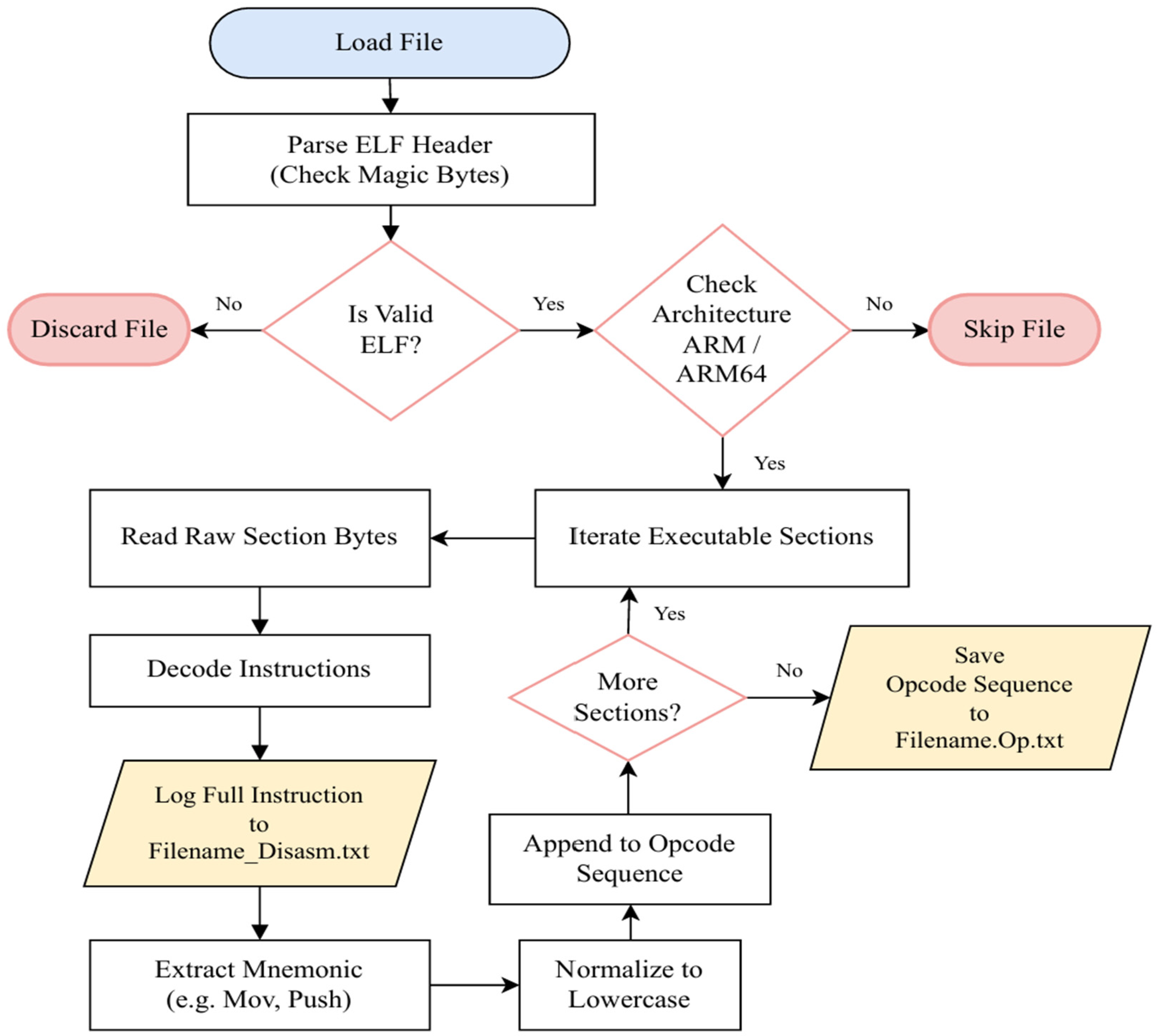
Figure 3 shows its core design and structure, with its details as follows:
The proposed disassembler encapsulates a robust system by integrating two libraries, Pyelftools and Capstone, to sequentially process machine bytes, thereby significantly reducing analysis time.
- 2.
Operational workflow
It begins with rigorous input validation using ELF magic bytes to ensure file integrity and filter out non-binary files, preventing dataset contamination. To maximize efficiency for the target environment, the system focuses exclusively on ARM architectures, given their dominance in the IoT ecosystem.
Figure 3 shows that the proposed disassembler uses a section-targeting method to find and extract executable payloads. This allows the system to capture relevant instruction sequences even from non-standard or obfuscated sections, ensuring a comprehensive feature set for subsequent analysis;
- 3.
Dual-output mechanism
This proposed disassembler is characterized by its dual-output process, producing two distinct data artifacts from each input ELF file, as illustrated in
Figure 3, both crucial for manual auditing and the subsequent feature engineering step.
As a result, the entire dataset is analyzed and disassembled using the proposed disassembler, as shown in
Figure 3. The computational efficiency of this pipeline was validated against Radare2, confirming that the entire process could be executed using the proposed disassembler. As detailed in
Table 4, the proposed disassembler demonstrates a substantial performance advantage: its speed is 9.10 times faster, and its source logic size is 415 times smaller than the task-equivalent components of Radare2, corresponding to improvements of 89% and 99.76%, respectively. By eliminating the need to install and configure external disassembler tools like Radare2, this method decreases system overhead and improves portability, resulting in an efficient and lightweight disassembler ideal for deployment on resource-limited IoT devices.
3.2.3. Opcode Feature Extraction
This process involves extracting meaningful features from raw data that are more representative and useful for the ML models. An informative and robust static feature called opcode is extracted from each disassembled file, which can effectively differentiate malware from a benign file because opcode captures program behavior by leveraging low-level information through analyzing IoT files statically. Opcodes are the machine language instructions that a CPU executes, which can be extracted during static analysis after disassembling the files into assembly code [
37], as done in this research.
Although the raw disassembly logs provide a granular view of the binary’s execution state, they contain memory offsets and register allocations that introduce stochastic noise into the learning process. As illustrated in the lower processing block of
Figure 3, the extraction methodology filters extraneous data to isolate the semantic logic (opcode sequence) of each disassembled file. Consequently, in this step, only opcodes (mnemonics, e.g., mov, ldr, and push) are extracted as features from the entire dataset and stored in a text format. This process ensures a noise-free, structure-preserving input for subsequent vectorization, capturing the fundamental execution flow of the binary without the overhead of dynamic execution.
3.2.4. Feature Engineering Using Opcode Frequency Profiling
The main goal of feature engineering is to transform extracted features into a suitable format that can be used by ML models and learn from them. The opcode frequency profiling technique is used to find a discriminative feature to effectively distinguish IoT malware from benign files due to its computational efficiency, which makes it more suitable for IoT devices. It provides a structured, numerical representation of a program’s low-level behavior, and its power is confirmed by many studies for IoT malware detection [
26,
29,
38].
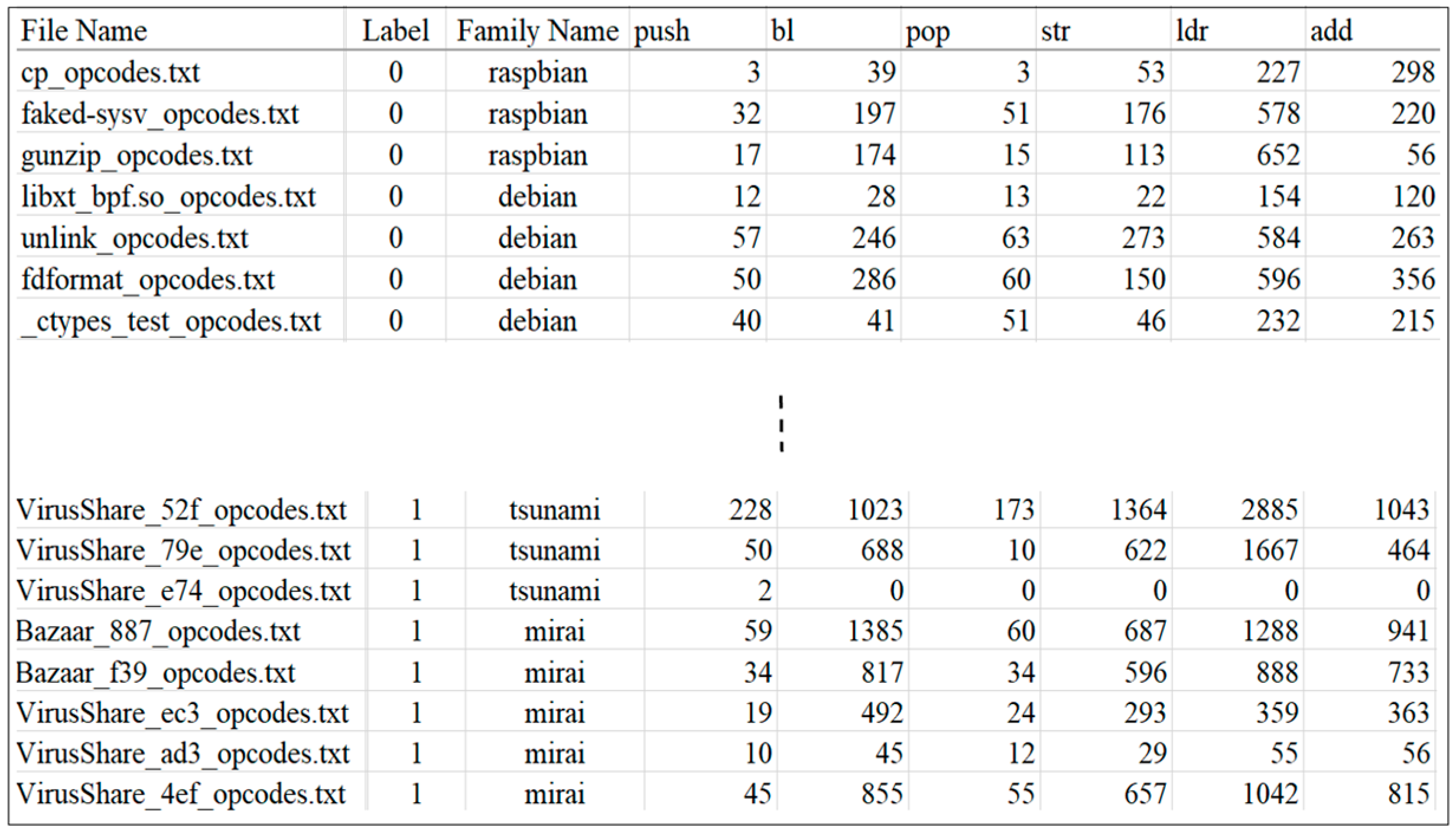
The opcode frequency profiling technique comprises two essential components. First, the raw opcode counting method based on 1-gram (unigram) analysis was applied to construct an absolute opcode frequency dictionary for each file. This approach is analogous to the Bag-of-Words (BoW) model commonly used in Natural Language Processing (NLP), where each opcode is treated as a token, and its absolute frequency (raw count) is utilized to represent the file. This method records the statistical autograph of the code by counting the occurrences of each unique opcode. This design choice renders the resultant features inherently robust against ‘dead code’ obfuscation. Unlike normalized relative frequencies, the absolute counts of functional opcodes are not diluted by the insertion of padding. Second, a feature vector generation method was implemented to convert the dictionaries into standardized, fixed-length numerical vectors. In these vectors, each dimension signifies a distinct opcode, with its value indicating the associated absolute frequency (raw count). Missed opcode values were automatically assigned to zero. Consequently, a final dataset was generated, comprising 1183 distinct opcode features, resulting in a structured, high-dimensional numerical representation of both malware and benign samples.
Figure 4 displays fifteen entries from the dataset generated after completing all of the steps of this phase.
3.3. Phase 3: Data Pre-Processing
It is a crucial stage before applying machine learning. It produces the appropriate information that the ML models can use to learn. In this research, the preprocessing phase includes two main steps, explained as follows.
3.3.1. Data Cleaning
Cleaning involves checking and removing duplicate data that could confuse evaluation and decision-making procedures. Data cleaning is essential, as it ensures that the ML models produce more accurate and reliable results. For this purpose, the file name and family name have been excluded from the entire dataset; see
Figure 4. Solely the label and opcode features were loaded for data cleaning. This step is used to clean the extracted feature vector from the duplicate records, confirming there is no duplicate or near-duplicate data in the train set and the test set. As an outcome, 5488 and 1092 duplicate records were found and removed from the train set and the test set, respectively. The remaining records from the cleaned sets within their classes’ distribution are revealed in
Table 5. The train set is denoted as op-train-set, while the test set is denoted as op-test-set for clarity. Since IoT malware detection is a binary classification problem, normally, classifier models have two classes, as in this research, where there are (Malware = 1) and (Benign = 0).
3.3.2. Feature Scaling Using Z-Score Normalization
Scaling the features is a crucial step of data pre-processing before training ML algorithms, especially for those that depend on distance calculations, like SVM or NN, to prevent feature dominance. Scaling enhances the ML algorithm’s performance because it guarantees that all features contribute equally to the model training. Z-score normalization, also known as Standard Scaler, is employed to scale the datasets utilizing Equation (1). This method converts the data to have a mean of zero and a standard deviation of one [
39].
where:
Zscaled: The data point’s scaled value;
x: The data point’s original value;
μ: The feature’s mean to which the data point belongs;
σ: The feature’s standard deviation to which the data point belongs.
After the completion of this phase, it is critical to note that only op-train-set serves as input for the feature selection and model training phases, whereas op-test-set is utilized to evaluate the eight trained ML models on real unseen data to ensure unbiased evaluation and confirm their performance and generalization ability.
3.4. Phase 4: Feature Selection (FS)
This phase is counted as a major one before classification procedures. FS is a process of selecting a subset of optimal features from the dataset and discarding irrelevant features that do not have discriminative power in distinguishing two different classes, such as the positive class (i.e., IoT malware file) and the negative class (i.e., IoT benign file), typically in the IoT malware detection era. FS’s critical role is not solely limited to dimensionality reduction but also evolves the models’ performance and avoids overfitting.
This phase explains the details of designing, proposing, and implementing two novel intelligent hybrid FS approaches. The VTH filter and LGBM-embedded methods are integrated for proposing the first FS approach named IHFS1, while the second FS approach is proposed through hybridizing the VTH filter and RFE-CV wrapper methods that utilize LGBM as an estimator, denoted as IHFS2. Before delving into the main structure of IHFS1 and IHFS2, the details of each FS method employed in this study are presented as follows:
The VTH is a renowned and extremely fast filter method. It prunes features based purely on statistical properties without involving any predictive model. It just calculates the variance for each feature using Equation (2) and removes all features whose variance does not meet the predefined threshold. By default, it removes all zero-variance features [
40].
where:
The RFE-CV is a wrapper feature selection method that uses the ML algorithm to select the most relevant and important features. To ensure its robustness, RFE-CV executes RFE in a cross-validation loop to find the optimal number of features that boost the model’s performance. RFE-CV scores each feature based on the ML estimator and iteratively eliminates features that do not maximize the model’s performance [
42,
43]. It automatically determines the optimal feature subset size due to its integration with cross-validation, thus eliminating the limitation of requiring the user to predefine the stopping point. Functioning as a greedy search strategy rooted in backward selection enables RFE-CV to systematically prune the feature space, avoiding an exhaustive exploration of feature combinations to efficiently converge toward a globally optimal solution [
44]. The RFE-CV process is initiated by training a base estimator using the complete feature set to rank feature importance or coefficient weights. The core recursive elimination mechanism involves iteratively retraining the model after systematically removing the feature(s) with the minimum importance weight. This continuous reassessment of feature relevance following the elimination of less critical attributes ensures a more thorough evaluation compared to single-pass approaches [
44]. Crucially, RFE-CV embeds this elimination process within a K-fold cross-validation loop to guarantee the stability and generalization of the selected feature set. This rigorous process executes the full recursive selection on each fold, measuring performance using a specified scorer (e.g., ROC-AUC) on the hold-out folds at every reduction step. The final feature set size is determined automatically by selecting the subset that achieves the maximum average cross-validated performance score across all K-folds, thus ensuring the final set is both minimal and maximally generalized [
45];
- 3.
LGBM
The LGBM is a gradient-boosting algorithm invented by Microsoft academics in 2017, which creates a model by generating a sequence of decision trees [
46]. The decision trees are trained to predict the target variable, like IoT malware and benign files. LGBM employs Gradient-based One-Side Sampling (GOSS) and Exclusive Feature Bundling (EFB) techniques to efficiently address challenges associated with high-dimensional feature spaces and imbalanced datasets. It has been widely employed across numerous classification tasks, including fraud detection, spam filtering, dark net traffic detection, etc., due to its efficiency, faster processing time, improved predictive accuracy, and less memory consumption [
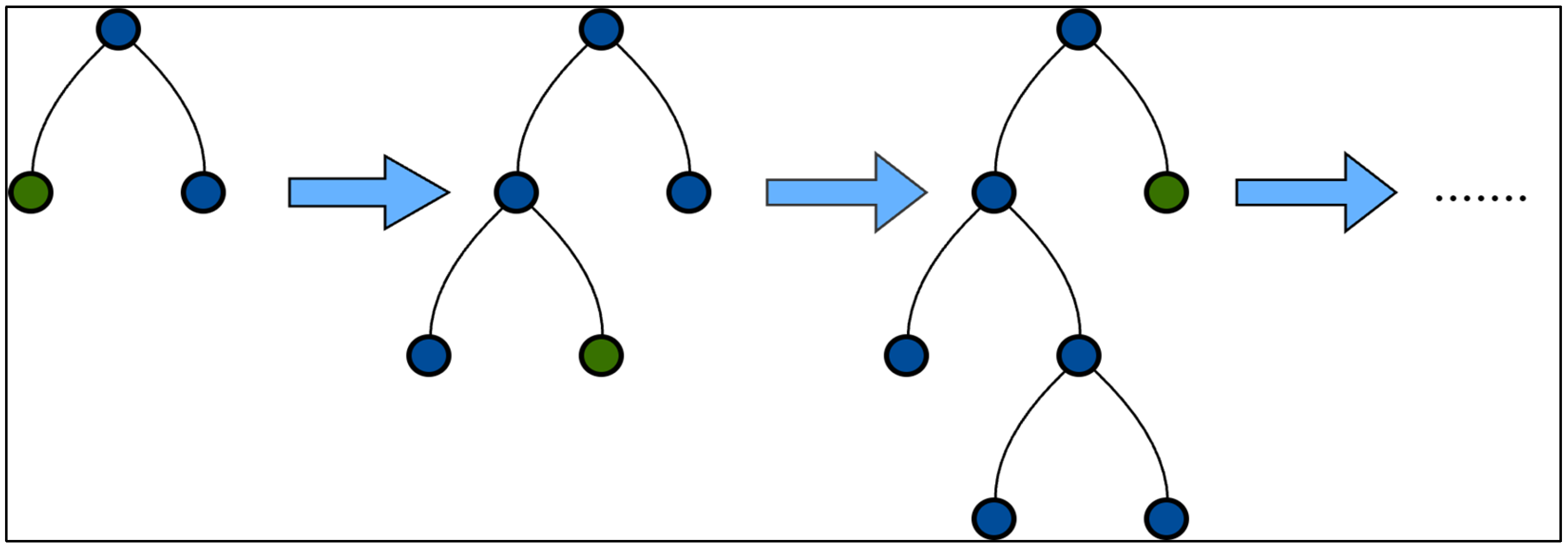
47]. Unlike traditional tree-based algorithms that employ a level-wise (depth-first) growth strategy, it utilizes a leaf-wise (best-first) growth mechanism, as revealed in
Figure 5. This approach prioritizes splitting the specific leaf that promises the largest residual reduction, resulting in a significantly minimized loss compared to level-wise methods. This targeted growth strategy provides superior loss reduction and enhanced model accuracy by converging faster on the most informative splits [
48].
The mathematical formulation of LGBM is centered on minimizing the objective function during the training process. The objective function, which is optimized to drive model performance, is expressed as follows:
where:
N: The number of samples in the dataset;
l: The loss function, measuring the difference between the true target values (Yi) and the predicted values (Y′i);
T: The number of leaves in the tree;
Ω (
Fi): The regularization term penalizing the complexity of the tree model [
48].
Table 6 presents the parameters within their setting values for each of the used FS methods to propose the novel FS approaches (IHFS1 and IHFS2).
3.4.1. Intelligent Hybrid Feature Selector 1 (IHFS1)
This feature selector is proposed based on hybridizing VTH and LGBM. VTH is utilized for its speed and effectiveness as an initial data cleaning step. This approach thereby reduced dimensionality and purged the dataset of noisy and uninformative features. Subsequently, LGBM was chosen for its inherent efficiency, reduced memory consumption, and high accuracy in scoring feature importance, leveraging its embedded FS capabilities. An IHFS1 outlines a two-stage process for selecting a discriminative feature set from a training dataset, specifically designed to robustly handle a binary classification problem with class imbalance.
As outlined in Algorithm 1, the procedure initiates by preparing the input data (i.e., op-train-set; see
Table 5) by extracting features (X_train) and the target variable (Y_train) and quantifying the class distribution (benign vs. malware instances). Crucially, to mitigate the impact of class imbalance on model training, a scale_pos_weight parameter is calculated for the LGBM classifier based on Equation (4). This parameter effectively rebalances the influence of the majority (malware) and minority (benign) classes by appropriately weighting the minority class during learning, leading to a more robust feature importance calculation. The first stage of IHFS1 involves VTH. This feature selector is initialized, and the variance of each feature is calculated. Then, if a feature’s variance in the dataset falls below a specified threshold, it is systematically removed. Many various thresholds were tested; 0.005 was selected because it was empirically validated as optimal via sensitivity analysis in
Appendix A and
Figure A1. This preliminary stage effectively filters out uninformative features that do not contribute to the predictive model’s performance and decreases the computational load for the next stage. Thereby, VTH created a refined feature subset, denoted as the variance-threshold feature set (X_VTH), by reducing dimensionality and eliminating potential noise. In the second stage, the LGBM classifier is configured with the
scale_
pos_
weight and trained on the (X_VTH) alongside the target variable (Y_train). After the training process, Algorithm 1 utilizes the LGBM’s inherent ability to compute feature importance scores, which quantify the relative contribution of each feature to the model’s predictive performance. These scores are then used to rank the features in descending order, facilitating the identification of the most influential features. Finally, a subset of the most impactful features is selected based on the predefined top
N feature criteria, which is set manually, as shown in Algorithm 1.
where
N_malware is the number of IoT malware instances, which is the majority class, whereas
N_benign is the number of IoT benign instances, which is the minority class in our train dataset.
| Algorithm 1: Intelligent Hybrid Feature Selector 1 (IHFS1) |
Input: D_train = {X_train, y_train}: Training dataset, τ: Variance threshold, N: retained feature’s no., Φ_LGBM: Hyperparameters for LGBM model
Output: F_selected (Optimal feature subset)
Procedure:
1. X ← D_train. features
2. y ← D_train. target
3. N_benign ← Count (y = 0)
4. N_malware ← Count (y = 1)
5. Spw ← Calculate class weight using Equation (4) to handle class imbalance
6. Compute variance vector σ2 for all features in X
7. Construct reduced feature set:
X_VTH = {f_j ∈ X | σ2(f_j) ≥ τ}
8. Configure LGBM model using Φ_LGBM and Spw
9. Train LGBM model on X_VTH: LGBM. fit (X_VTH, y)
10. Extract feature importance scores based on gain:
I = {(f_i, s_i) | f_i ∈ X_VTH}, where s_i denotes the importance score of f_i feature
11. I_sorted ← Sort (I, descending by s_i)
12. F_selected ← {f_i | (f_i, s_i) ∈ I_sorted [1…N]}
13. Return F_selected |
3.4.2. Intelligent Hybrid Feature Selector 2 (IHFS2)
This feature selector is proposed depending on a hybrid approach grouping VTH and RFE-CV with LGBM as an estimator. It is more advanced than IHFS1 and specifically designed to select an optimal subset accurately with class imbalance handling. In IHFS2, RFE-CV is used due to its accuracy and automatically tunes the number of selected features by fitting an RFE selector, thereby avoiding the manual setting of the top N features criterion required by Algorithm 1.
As outlined in Algorithm 2, the procedure commences with the first stage, which is the same as steps (1–7) of Algorithm 1 until the X_VTH is obtained, which includes a subset of selected features after a VTH method has been completed. The core of IHFS2 resides in its second stage, which employs RFE-CV with LGBM. The LGBM classifier, configured with the pre-calculated scale_pos_weight to address class imbalance, serves as the base estimator within the RFE-CV framework. RFE-CV iteratively trains the LGBM model, assesses feature importance, and removes the least important features based on the Area Under the Receiver Operating Characteristic Curve (ROC-AUC) metric, thereby converging on an optimal subset of features. The selection of the optimal feature subset is rigorously guided by the ROC-AUC score, which is particularly better suited for an imbalanced dataset. This evaluation is performed through the RFECV_k parameter, which is a stratified K-fold cross-validation splitting strategy that preserves the percentage of samples for each class across all folds. This ensures that the chosen features not only maximize predictive performance but also exhibit robust generalization across different data partitions, yielding a final set of highly relevant and discriminative features. Another critical parameter that controls the efficiency of the RFE-CV method is RFECV_Step, which removes the least important number of features in each iteration. By default, it is one, but it needs to be tuned based on the nature of the problem that needs to be solved. As shown in
Table 6, the RFECV_Step parameter value is set to 40 based on a preliminary sensitivity analysis (detailed in
Appendix A and
Figure A2) to speed up the elimination process and explore the optimal trade-off between feature compactness and the model’s efficacy. This configuration facilitated the development of a highly precise and computationally efficient ML detector that is ideal for implementation on resource-limited IoT devices.
| Algorithm 2: Intelligent Hybrid Feature Selector 2 (IHFS2) |
Input: D_train, τ, Φ_LGBM, RFECV_k: Number of CV folds, RFECV_Step: Number of features to be removed in each iteration;
Output: F_selected (Optimal feature subset)
Procedure:
1. X ← D_train. features
2. y ← D_train. target
3. N_benign ← Count (y = 0)
4. N_malware ← Count (y = 1)
5. Spw ← Calculate class weight using Equation (4) to handle class imbalance
6. Compute variance vector σ2 for all features in X
7. Construct reduced feature set:
X_VTH = {f_j ∈ X | σ2(f_j) ≥ τ}
8. Initialize LGBM estimator using Φ_LGBM and Spw
9. Iterative RFE-CV Process:
Initialize Score_history ← ∅
While |X_VTH| > 0:
Initialize CV_scores ← ∅ // ROC-AUC value obtained from the LGBM estimator
Stratified partitioning of {X_VTH, y} into RFECV_k folds
For i = 1 to RFECV_k:
Split {X_VTH, y} into Train(i) and Validation(i)
Train LGBM on Train(i)
Score(i) ← Calculate ROC-AUC on Validation(i)
Append Score(i) to CV_scores
End For
Mean_Score ← Average (CV_scores)
Append (Mean_Score, X_VTH) to Score_history
Train LGBM on full {X_VTH, y}
Compute feature importance for all f ∈ X_VTH
F_remove ← Identify bottom RFECV_Step features with lowest importance
X_VTH ← X_VTH \ F_remove
End While
10. F_selected ← arg maxX_VTH {Mean_Score ∈ Score_history}
11. Return F_selected |
In this research, only the op-train-set is fed to the FS phase, as clarified in
Figure 1. First, the high-dimensional training dataset containing 1183 features is processed by the IHFS1. As a result, 50 opcode features are identified as optimal, and a new low-dimensional dataset is constructed, representing a substantial reduction in dimensionality. This outcome demonstrates the effectiveness of IHFS1 in selecting the most discriminative features while minimizing computational overhead and preserving the model’s performance.
Subsequently, the same feature set was processed by IHFS2, which identified only 23 opcode features as optimal out of the original 1183 features. The obtained outcomes yield a significant reduction rate in the dimension of the original training dataset. Also, it is validated that both proposed FS approaches, IHFS1 and IHFS2, serve as an efficient dimensionality reduction tool.
The primary goal of this feature reduction (from 1183 to 50 and 23 features using IHFS1 and IHFS2, respectively) was to significantly reduce the computational burden, thereby decreasing both model training time and subsequent inference time, while simultaneously preserving or improving model accuracy.
To further validate their efficacy within two selected feature subsets, we trained and tested several famous supervised ML models, as explained in the next phase.
3.5. Phase 5: Evaluation Using Supervised Balanced ML Models
This phase is divided into training and evaluating steps. It demonstrates the methodology of training and evaluating eight supervised balanced ML models on three various datasets for IoT malware detection. The main objective of training ML models was to comprehensively:
Assess the efficiency and accuracy of both proposed feature selectors;
Evaluate the discriminatory power of the selected feature subsets in distinguishing IoT malware from IoT benign files;
Identify the robust and fast detector model for detecting IoT malware that belongs to famous families, i.e., Mirai, Gafgyt, and Tsunami, which are major threats for resource-constrained IoT devices.
This evaluation was done through training three balanced tree-based models (LGBM, DT, and RF), two balanced linear-based models (LR and SVM), and three balanced probabilistic models (Complement Naïve Bayes (CNB) and Multinomial Naïve Bayes (MNB), and GNB). A brief description of each one is provided as follows:
3.5.1. Training Supervised Balanced ML Models
The first model was LGBM due to having several exceptional benefits, as discussed in the aforementioned phase. In this phase, the LGBM classifier was also configured with the scale_pos_weight parameter, as employed during the FS stage to address the class imbalance.
The second model was RF, which is an ensemble-learning method that uses bagging techniques to grow trees to their maximum extent. Each learned tree is a weak learner, but when combined, a strong model is built. The overall prediction is based on the majority votes from all weak learners. RF offers strong generalization capabilities and robustness against overfitting and can handle large datasets with high dimensions [
42,
46]. Its resilience to noise and high accuracy make it a reliable choice for IoT malware detection [
25,
30,
31].
The third model was DT, which utilizes a tree-like structure with branches and leaves for classification rules. Information gain is used to select optimal attributes during training. DT offers high interpretability for malware detection but has an overfitting problem, which is resolved by RF [
49]. DT is selected due to simplicity and minimal inference size, which makes it a good candidate for the construction of lightweight anti-malware for IoT devices;
LR is frequently used for binary classification tasks and applies the sigmoid function or its variations to confine the output values within the range of [0, 1]. A value closer to one signifies a higher probability of belonging to a particular class [
42,
50]. The selection of this classifier was primarily motivated by its computational efficiency.
Then, SVM was trained using a linear kernel. This classifier is primarily characterized by its ability to construct a separating hyperplane that maximizes the margin between classes in the feature space [
51]. SVM is effective for IoT malware detection, intrusion detection, etc., because of its strong theoretical foundation, good generalization performance, and robustness in identifying complex boundaries between benign and malicious [
49];
First, the CNB was trained, which is an improved variation of Naive Bayes (NB), particularly designed for imbalanced datasets. It calculates probabilities from the complement of each class based on the equation provided in [
52]. It is chosen for its intrinsic capacity to resolve imbalance issues.
Second, MNB, a trained form of NB, is widely used for spam detection and sentiment analysis due to its simplicity and effectiveness. It assumes a multinomial distribution based on Bayes’ theorem, making it effective for discrete features and counting [
42,
46]. Its computational speed makes it ideal for IoT environments.
Lastly, GNB was trained, which is the popular type of NB, and is applicable when the features follow a continuous Gaussian (normal) distribution [
52]. It offers simplicity and computational speed due to having a smaller number of parameters, making it suitable for IoT devices. Despite its nature, which works well with continuous data, the experimental results showed that GNB also works well with discrete data, which is a critical finding obtained through this study.
Upon completion of the feature selection phase, the eight aforementioned balanced ML models were trained on 1 high-dimensional dataset and 2 low-dimensional datasets, including 1183, 50, and 23 features, respectively. This experiment is quite significant, which depicts the efficiency of the proposed FS approaches and shows how proposing an efficient FS approach affects the ML model’s training and testing times, as well as accuracy, which are extremely critical criteria that must be considered when developing an efficient IoT malware detection system, ensuring alignment with the inherent constraints and operational nature of IoT devices. Before training ML models, each dataset is partitioned into distinct training and validation sets using StratifiedKFold cross-validation. This partitioning is conducted with two different fold configurations (k = 5 and k = 10) to ensure the meticulous preservation of class proportions within each subset. Stratified sampling is paramount for imbalanced datasets, as it prevents the models from being biased and performing well on the majority class but poorly on the minority class. In StratifiedKFold cross-validation, when k is equal to 5, the dataset is segmented into 5 equal sets; 4 sets (80%) of the dataset are used for training the model, while 1 set (20%) is used for the model’s evaluation in each fold. However, when k is equal to 10, the dataset is divided into 10 equal segments. Nine sets (90%) are used for training the model, while - one set (10%) is used for the model’s evaluation in each fold. In this study, an additional solution for addressing the class imbalance problem involved configuring LR, SVM, RF, DT, GNB, and MNB by setting the class_weight parameter to ‘balanced’. This parameter prevents these models from biasing toward the major class and leads them to learn equally on both classes, as validated in
Section 4. In addition, the LGBM is configured via scale_pos_weight, whereas CNB naturally handles class imbalance without any specific parameter. These algorithmic approaches were selected and prioritized over the Synthetic Minority Over-sampling Technique (SMOTE) to preserve the semantic integrity of the benign samples and avoid the computational overhead of processing synthetic data. Furthermore, the strength of the used strategy is empirically confirmed by the Confusion Matrix evaluation as validated in
Section 4. Hyperparameters for all eight ML models were systematically optimized using a Grid Search approach over a predefined parameter space to ensure that the resulting classifiers achieved maximal performance and stability.
Table 7 describes the parameter tuning for each trained balanced ML model to be nominated as an effective IoT malware detector after evaluating on unseen samples.
Moreover, the random state and shuffle parameters were 42 and true, respectively, for all proposed balanced ML models mentioned in
Table 7.
3.5.2. Evaluating Trained ML Models Using Performance Metrics
This sub-subsection demonstrates the picked metrics to evaluate the effectiveness of the ML models during training and after they are tested on unseen samples. This evaluation validates the efficacy of the proposed FS approaches (IHFS1 and IHFS2) and the power of the selected feature sets. After the eight balanced ML models were trained on three different feature sets, as explained earlier, their performances were assessed through several metrics using the op-test-set. This dataset has never been seen before by the models and has not been involved during the training and validation phases.
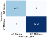
The picked metrics that were mostly used in the IoT malware detection era were accuracy, precision, recall, F1-score, and the confusion matrix. Moreover, in this research, the dimensionality reduction rate for the original dataset after feature selection, alongside training and prediction times for each trained ML model, is considered. All the metrics were carefully picked to accurately reveal the power of the selected feature sets and show the significance of the feature selection phase.
Accuracy is defined as the ratio of correctly classified instances to the total number of instances in the dataset. Precision quantifies the proportion of samples predicted as malware that are truly malicious, reflecting the model’s reliability in positive predictions. Recall, also known as sensitivity or true positive rate (TPR), measures the proportion of actual malware samples that are correctly identified by the model. The F1-score, which is particularly informative in the presence of class imbalance, represents the harmonic mean of precision and recall, balancing both false positives and false negatives.
Furthermore, the confusion matrix offers a comprehensive breakdown of classification outcomes, including four components:
True Positives (TP): IoT malware samples correctly identified as malicious;
True Negatives (TN): IoT benign samples correctly classified as non-malicious;
False Positives (FP): IoT benign samples incorrectly classified as malicious;
False Negatives (
FN): IoT malware samples incorrectly classified as non-malicious [
27].
Lastly, dimensionality reduction rate (
Drr) is a very critical measure to validate the efficiency of the proposed FS approaches, which measures the percentage of features that were removed from the original dataset after a feature selection was applied [
53]. Accuracy, precision, recall,
F1-
score, and
Drr are calculated using Equations (5)–(9), respectively [
16,
42,
53].
3.6. Statistical and Computational Analysis
To assess both the consistency of the ML models’ performance and the statistical significance of the computational savings achieved by the feature reduction via IHFS1 and IHFS2, a rigorous analysis was conducted.
- 1.
Consistency and reporting
To reduce variability and enhance the reliability of the findings, all model training and testing procedures were repeated across 20 independent runs. Comparisons were conducted between the initial feature set (1183 features) and the optimized feature sets obtained via IHFS1 (50 features) and IHFS2 (23 features). The stability of the reported metrics, including training time and inference time, was quantified using descriptive statistics. All data are presented as the mean (µ) plus or minus the standard deviation (SD) to illustrate the central tendency and dispersion, respectively.
Crucially, the detection metrics (accuracy, precision, recall, and F1-score) remained perfectly stable across all 20 independent runs for both the initial and optimized configurations, confirming that the measurement process was deterministic and that the feature reduction successfully optimized computational speed without introducing unwanted performance variability;
- 2.
Validation of computational efficiency
The core hypothesis that feature reduction significantly decreases computational cost was validated using inferential statistics. A two-sample independent t-test (Welch’s t-test), which is robust under the assumption of unequal variances, was performed to determine the statistical significance of the difference between the mean times recorded for the initial and the optimized feature sets. This test was applied separately to compare the following:
The mean training time of the initial (1183 features) versus the two optimized groups (50 features via IHFS1 and 23 features via IHFS2);
The mean inference time of the initial (1183 features) versus the two optimized groups (50 features via IHFS1 and 23 features via IHFS2).
The criterion for determining statistical significance in all comparisons was conventionally set at p < 0.05.
4. Results and Discussion
In this section, the environmental setup’s properties and all the investigational outcomes obtained from proposing FS approaches and eight balanced ML models are discussed in detail.
4.1. Environment Setup
In this investigation, three different environments were utilized, including local isolated, Colab, and simulated.
First, a local isolated environment is set up on the personal computer (PC) running Windows 10 (64-bit) with RAM (16 GB) and a Core i7 (1.8 GHz) CPU. This isolated environment is created using a virtual machine (VirtualBox) for conducting phase 1 (IoT malware dataset collection and preparation) and phase 2 (IoT static malware analysis) to prohibit any infections, since working with malicious files is risky. Second, the Colab (CPU) environment was utilized for employing the other phases (3, 4, and 5). Third, a high-fidelity simulated environment is built using a native ARM64 architecture host to test the proposed IoT malware analysis and DT-based detection engine in real-world edge-computing situations. The simulated environment is configured with specific limitations to mimic the hardware parity of resource-constrained IoT devices (e.g., Raspberry Pi), strictly partitioned to 1.0 GiB of physical RAM, with a disabled memory swap and 1 virtual CPU core, to ensure that all metrics represent local CPU and memory throughput without the influence of secondary disk paging. According to the results, the DT model was the fastest and most accurate, so it was selected. And the test phase was repeated with this model in the simulated environment.
Finally, all the phases of this research were entirely implemented using Python version 3.11.13 in all environments except IoT malware dataset collection, alongside several libraries, namely, Capstone 5.0.6, Pyelftools 0.32, NumPy 2.0.2, Pandas 2.3.3, Seaborn 0.13.2, Matplotlib 3.9.4, SciPy 1.13.1, and Scikit-learn 1.6.1.
4.2. Experimental Results and Critical Analysis
As explained previously, the final generated datasets in phase 3 were op-train-set and op-test-set, representing 80% and 20% of ARMIoTDS-25, respectively. These ratios were utilized in all the experiments of this research. Accordingly, the op-train-set is used for proposing FS approaches and training eight balanced ML models, while the op-test-set is used solely for testing and evaluating the power of selected feature sets and the performance of all trained ML models on real-world data. To validate the experiments, a stratified 5- and 10-fold cross-validation was applied in proposing all balanced ML models. Eventually, the overall performance of the eight proposed ML models is comprehensively assessed using performance metrics along with training and inference times.
4.2.1. Results Achieved After Feature Selection Using IHFS1 and IHFS2
Figure 6 illustrates the impact of IHFS1 and IHFS2 on the initial dataset in terms of dimensionality reduction rate, the retained features ratio, and the number of features before and after applying the proposed FS approaches with their power in handling the dimensionality reduction issue.
In addition, both IHFS1 and IHFS2 demonstrate an exceptional efficiency through significantly reducing the dimensionality of the original feature space. IHFS1 yields a reduced dataset, comprising approximately 4.23% of the initial features, while IHFS2 produces another reduced dataset, retaining only 1.94% of the original features. These results highlight the efficiency of each proposed FS approach in preserving informative features while minimizing feature space complexity and computational overhead.
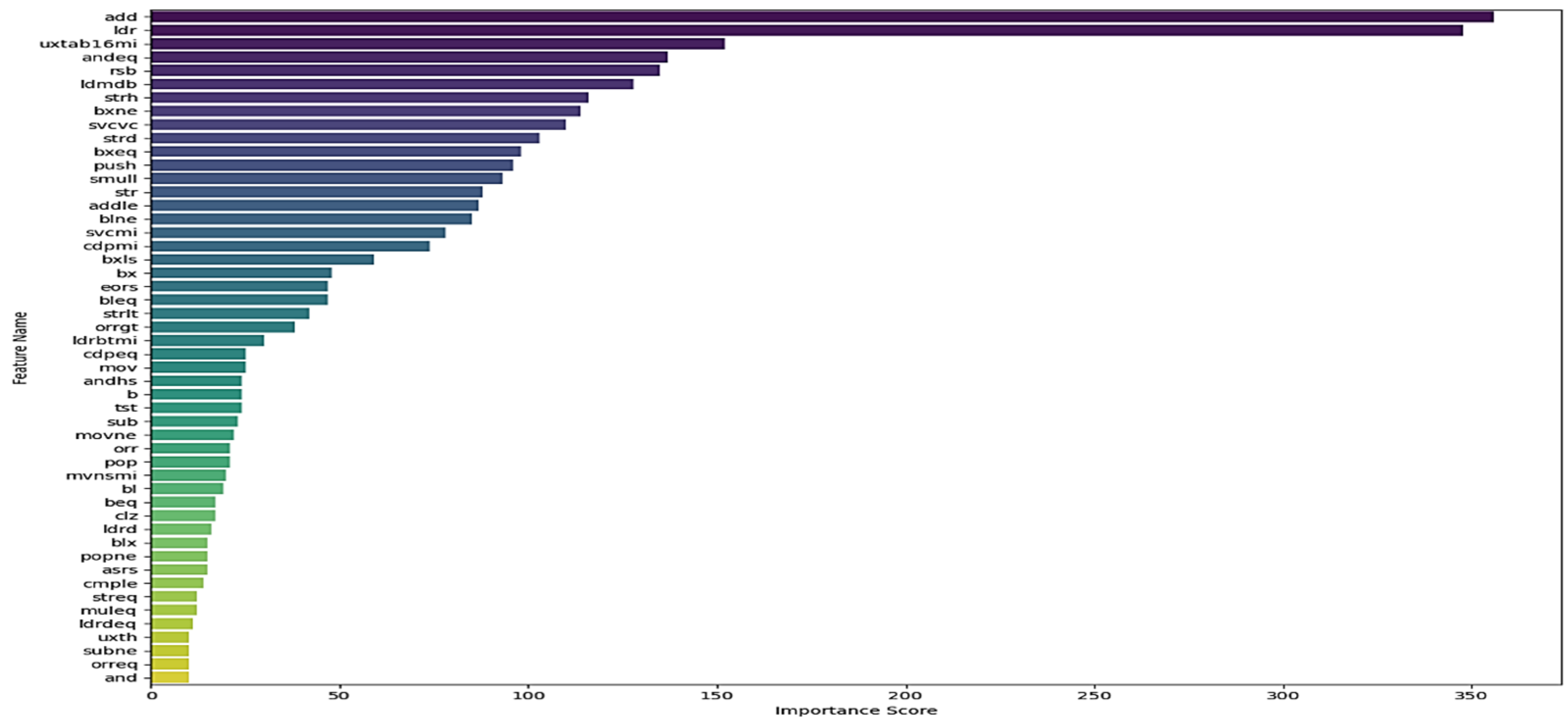
Figure 7 presents the 50 discriminative opcode features alongside their importance scores selected using the IHFS1, where the Y-axis represents the names of the selected features and the X-axis shows their importance score based on the LGBM classifier.
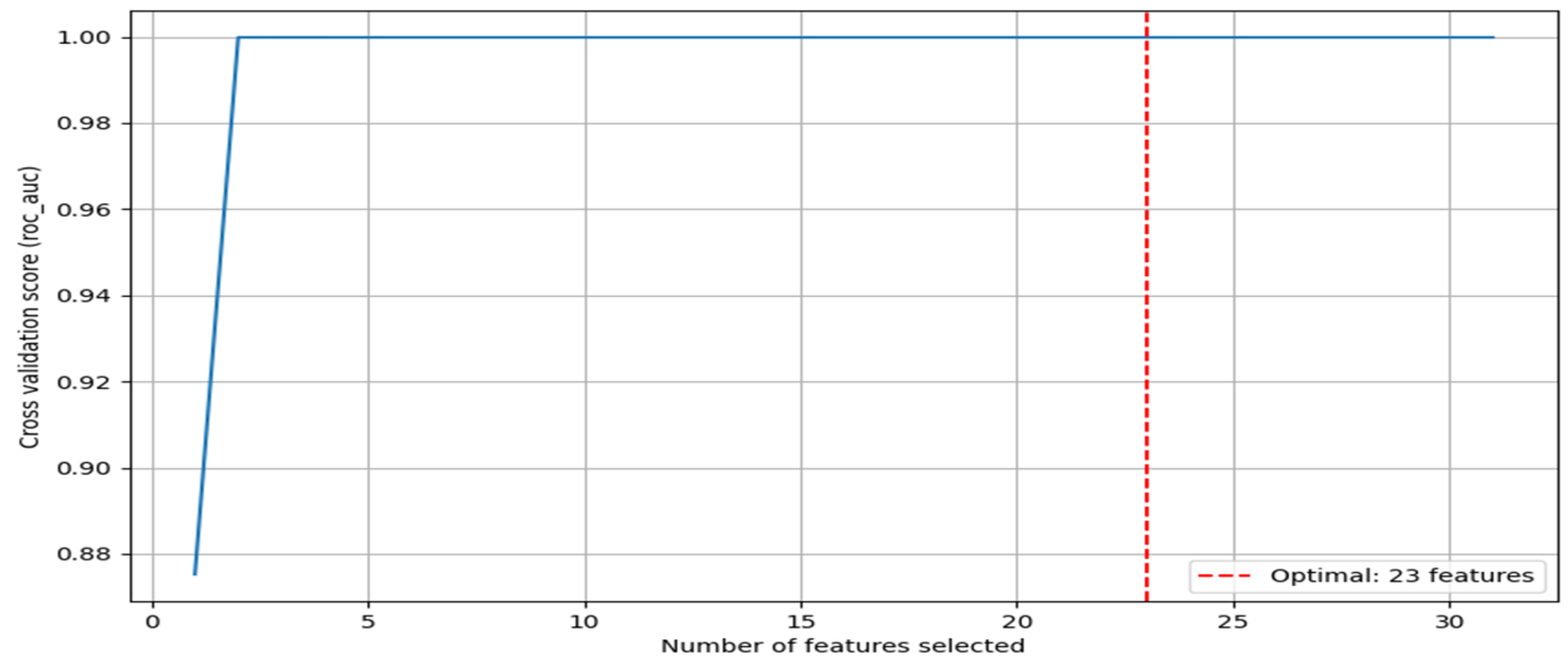
The performance of IHFS2’s second stage is presented in
Figure 8, once the RFE-CV process is started using LGBM as the estimator. The figure depicts the selection of a 23-optimal feature subset, alongside the ROC-AUC score recorded at each iteration.
As depicted in
Figure 8, the LGBM model achieved a perfect cross-validation ROC-AUC score close to one from approximately three features. This high performance, even with a limited feature set, is characteristic of powerful gradient-boosting models like LGBM when strong predictive signals are present in the data. Despite achieving perfect performance with fewer features, the RFE-CV process ultimately identified 23 features as optimal. This occurred because the LGBM model’s performance remained consistently at a perfect classification score of nearly one as more features were added up to this point.
In this scenario, RFE-CV selected the largest subset of features that maintained the maximal cross-validation score, as adding these features did not degrade the model’s performance. As a consequence, 23 features were identified as optimal based on the ROC-AUC score.
Figure 9 describes 23 discriminative opcode features selected with their importance scores using IHFS2.
Figure 7 and
Figure 9 demonstrate that the selected feature sets are predominantly composed of functionally critical opcodes. The 50 feature set includes critical indicators such as add, ldr, and uxtab16mi, while the 23 feature subset focuses on core operations like svc, str, and eors. Beyond their statistical significance, these feature sets provide inherent resilience against common obfuscation techniques and compilation variance as follows:
The proposed disassembler is designed to analyze binary structures systematically to identify executable instructions, including those located in non-standard sections or obscured by junk byte insertion. This comprehensive extraction ensures that all semantic content of the malware is captured, despite its attempts to conceal it. The generated feature vectors precisely represent the file’s operational functionalities, making the detector robust against spatial layout alteration methods;
- 2.
Resilience to dead code insertion
The methodology employs raw opcode counting, allowing the selected feature sets (50 features via the proposed IHFS1 and 23 features via the IHFS2 approaches) to function as passive filters. Padding opcodes such as ‘nop’ were excluded because of their insignificant importance scores, ensuring that the insertion of benign dead code does not dilute the feature vectors. The absolute magnitude of malicious indicators, such as the high count of uxtab16mi or ldr shown in
Figure 7, remains statistically dominant even in the presence of injected noise;
- 3.
Resilience to instruction reordering
Obfuscation techniques rely on swapping or shuffling instructions specifically targeting sequence-dependent models (e.g., N-grams where N > 1 or CFG). However, the utilized 1-g (Bag-of-Words) model is inherently permutation-invariant. Since the feature vector relies solely on raw opcode counts rather than their sequential arrangement, reordering the instructions results in a mathematically identical feature vector, ensuring the classification score remains unaffected;
- 4.
Resilience to compilation variance
Although compiler optimization levels can modify the instruction’s sequencing, they cannot remove the essential opcodes required by the ARM Application Binary Interface (ABI). Operations like system calls (svc), memory manipulation (ldr, str, ldmdb), and encryption processes (eors) in the 23 features, and structural markers like push/pop for stack management in the 50 features, remain invariant across different compilers.
4.2.2. Results Attained After Evaluating IHFS1 Using Balanced ML Models
In this part, the strength of the reduced feature subset that was selected using IHFS1 is revealed via training and testing eight balanced ML algorithms steadily for IoT malware detection. Furthermore, its performance is compared with the initial feature set using evaluation metrics. Across all experiments, the eight models were trained using both 5-fold and 10-fold cross-validation. However, due to the extensive volume of results, only the outcomes from 10-fold cross-validation are reported. As a consequence, the low-dimensional dataset led to a significant reduction in all of the ML models’ training and prediction times, which is validated by statistical significance testing. Thus, identifying a fast and accurate ML detector for IoT malware.
In the first experiment, eight proposed ML models were compared in terms of picked performance metrics. At first, we compared the models regarding training and testing accuracies. Training accuracy is obtained once the models are trained on 1183 features before feature selection and the 50 optimal features that were selected by IHFS1. However, the testing accuracy is attained after assessing the eight trained models on the op-test-set. This test aimed to present the efficiency of IHFS1 regarding accuracy because, generally, reducing the number of features affects the model’s accuracy. However, despite using only 50 optimal features for training 8 ML models, a high accuracy was achieved, with improvements observed across all proposed ML models, particularly in the training accuracy of GNB, which improved from 0.9556 to 0.9958, as shown in
Table 8.
Furthermore,
Table 8 presents the performance of the eight trained ML models in terms of testing accuracy on unseen data. This experiment depicted that the testing accuracy of LGBM, DT, and GNB was improved when they were trained on 50 features, whereas the testing accuracy of RF, CNB, MNB, and LR was slightly better when they depended on 1183 features. It is critical to note that SVM’s testing accuracy was stable, but a significant improvement has been seen in GNB’s testing accuracy, which enhanced from 0.9587 to 0.9957.
This test has shown that the accurate detector is RF, with a testing accuracy of 99.91%, and outperformed other detectors when 1183 features were used. However, both RF and LGBM were accurate detectors and gained the same testing accuracy of 99.87% once they were trained on 50 optimal features. This experiment confirmed that the first proposed FS approach (IHFS1) accurately selected highly informative features that improved the ML model’s accuracy, as depicted in
Table 8.
In addition to accuracy, other metrics such as precision, recall, and F1-score are critical for showing the robustness of the trained ML models’ performance on unseen data for IoT malware detection, as presented in
Table 9. Overall, the models achieved a high rate. Therefore, both LGBM and RF demonstrated robustness after being trained on 50 features, surpassing other models by generating low false alarms (high precision of 99.94%), detecting all actual IoT malware (high recall of 99.88%), and achieving a 99.91% F1-score. These results demonstrated the perfect handling of the class imbalance issue and the selection of highly discriminative features by IHFS1.
In the second experiment, eight proposed ML models were benchmarked in terms of mean training time and mean testing (inference) time, measured in seconds using a Colab (CPU) instance to establish a performance baseline. The primary objective was to evaluate the computational efficiency gain achieved by the IHFS1 methodology, which reduced the feature space from the initial shape of (8150, 1183) to the optimized shape of (8150, 50), consequently improving both training and inference time performance. To confirm that the observed time differences are statistically meaningful, validation was performed using an independent-samples
t-test. The detailed results, including the mean, standard deviation, and
p-value, are shown in
Table 10.
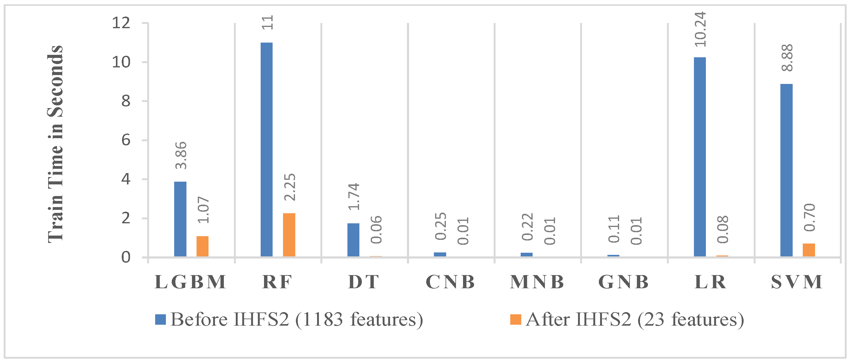
The mean training time was measured after each of the eight ML models was trained 20 times on both the full 1183 feature set and the reduced 50 feature set, as revealed in
Table 10 and
Figure 10. The feature reduction that was obtained using the proposed IHFS1 FS approach efficiently and significantly decreased the mean training time of all models.
Specifically, the RF model’s mean training time was substantially reduced from 11 s to 3.92 s, while the LR model experienced the most dramatic improvement, decreasing from 10.24 s to a mere 0.17 s. Significant gains were also observed sequentially for SVM, LGBM, DT, CNB, MNB, and GNB. As a direct consequence, the IHFS1 methodology reduced the total aggregate mean training time from 36.30 s to just 5.93 s. This outcome represents a 6.12 times acceleration in the training process, equating to an 83.69% reduction in training time, with the statistically significant difference confirmed by p < 0.001 for all models.
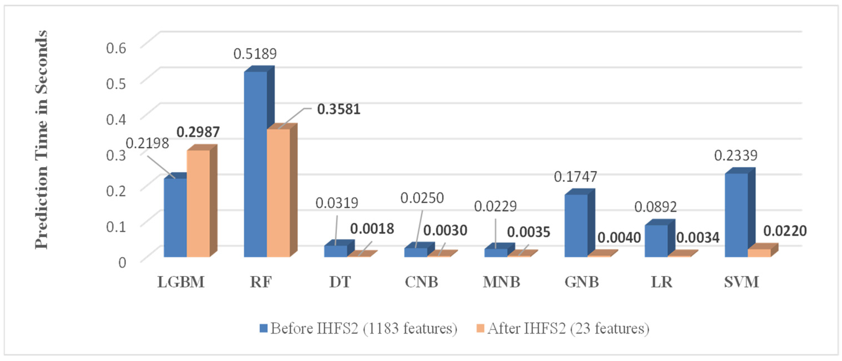
Second, the testing time (also referred to as the prediction or inference time) was measured in seconds after the trained models were evaluated on unseen samples, as demonstrated in
Table 10 and
Figure 11. Notably, the reported testing time solely represents the classification step without disassembly, feature extraction, and feature engineering steps. Inference time is a crucial criterion for identifying a time-efficient IoT malware detector, directly indicating its deployment feasibility and speed in real-time detection scenarios.
Based on this experimentation, the MNB model was the fastest when the full 1183 features were used, requiring only 0.0229 s to generate predictions. However, the DT model emerged as the fastest detector when using the reduced 50 features, taking solely 0.0026 s to complete the prediction. In contrast, the RF model, despite its significant training time reduction, revealed the slowest overall inference performance at 0.4858 s. This test confirmed that IHFS1 efficiently optimized the models’ inference time. For instance, the SVM model’s mean prediction time decreased dramatically from 0.2339 s to 0.0265 s. Consequently, IHFS1 validated its efficiency by reducing the total aggregate mean test time from 1.3163 s to just 0.7850 s. This results in the testing process being 1.68 times faster, representing a 40.37% reduction in testing time, with all models showing a statistically significant difference of p < 0.001.
4.2.3. Results Attained After Evaluating IHFS2 Using Balanced ML Models
This part validates the efficacy of the 23 optimal features selected using the IHFS2, demonstrating their impact on model performance and efficiency.
In the first experiment, the eight trained ML models were compared based on evaluation metrics. Initially, the 8 ML models’ training accuracies were compared once they were trained on 1183 and 23 feature sets. The goal of this test was to demonstrate the efficacy of IHFS2 in regard to accuracy, as the number of features was reduced further by IHFS2 than by IHFS1. However, despite using just 23 optimal features, high accuracy was still gained. This indicated that IHFS2 accurately selected the most discriminative features, resulting in the accuracy improvement of almost all the proposed ML models, except LR’s accuracy, which diminished slightly from 0.9962 to 0.9961. This test identified that GNB’s training accuracy escalated dramatically, from 0.9556 to 0.9960, when the features were reduced from 1183 to 23 features, as highlighted in
Table 11. The accurate model was RF when trained on both feature sets and surpassed other detectors.
Additionally,
Table 11 presents the test accuracy performance of the eight trained ML models, which was achieved after being tested on unseen data. This assessment showed that the accurate model is RF across two various feature sets for detecting IoT malware and distinguishing it from IoT benign due to achieving high accuracy, which was between 99.91% and 99.87% on the unseen samples, outperforming the other evaluated models. Likewise, DT gained 99.87% accuracy with 23 features. Once more, a dramatic improvement can be seen in GNB’s test accuracy, from 0.9587 to 0.9961, when the features were reduced. This validated that IHFS2, which hybridized VTH and RFE-CV with LGBM, dynamically and accurately selected informative features, which enhanced the models’ training accuracy and preserved their testing accuracy using merely 23 optimal features. For example, RF and DT based only on 23 opcode features operate as a robust IoT malware detector due to achieving a high and identical accuracy rate of 99.87% on the unseen data.
Furthermore,
Table 12 reveals the obtained test ratios of precision, recall, and F1-score for all models. Overall, the models gained an exceptional rate. These attained outcomes proved that IHFS2 selected a highly optimal and discriminative feature set. Therefore, RF was a robust detector again and outperformed other detectors in terms of generating low false alarms (high precision of 99.94%), catching all actual IoT malware (high recall of 99.88%), and having a 99.91% F1-score. In addition, this test proved that the class imbalance issue was handled perfectly using balanced ML models.
In the second experiment, the mean training time for eight ML models was benchmarked using both the large 1183 feature set and the highly reduced 23 feature set selected by the IHFS2. The comparison confirmed that the time differences were statistically significant (
p < 0.001) across all models. Specifically, the training times for RF, LR, and SVM saw the most significant reductions, decreasing from 11 s, 10.24 s, and 8.88 s to just 2.25 s, 0.08 s, and 0.70 s, respectively. This performance gain was followed by notable reductions in LGBM, DT, CNB, MNB, and GNB, as presented in
Table 13 and
Figure 12. This feature reduction accelerated the RF, LR, and SVM classifiers by approximately 4.89, 128, and 12.69 times, respectively. Consequently, the total aggregate mean training time across all models was reduced from 36.30 s to only 4.19 s, making the overall training process 8.66 times faster. This represents an 88.46% reduction in training time.
Second, the prediction (inference) time was measured to determine which models are suitable for fast IoT malware detection. Statistical significance testing confirmed that the time differences were statistically significant (
p < 0.001) for the optimized models compared to their initial counterparts. Overall, utilizing the 23-feature set significantly diminished the models’ prediction times, with the exception of LGBM. Based on the outcomes presented in
Table 13 and
Figure 13, the DT model emerged as an exceptionally fast detector, classifying 2323 samples in just 0.0018 s and achieving an acceleration of 17.72 times over its initial performance. While RF maintained high detection accuracy, it was the slowest model during the prediction phase. Furthermore, significant inference speed enhancements were observed for SVM and GNB, with their times dropping from 0.2339 s to 0.0220 s and 0.1747 s to 0.0040 s, respectively. This resulted in the SVM classifier being accelerated by nearly 10.63 times. These enhancements in inference speed are crucial for the practical deployment of the proposed system on IoT devices, where low latency is paramount. Ultimately, IHFS2 proved its high efficiency by diminishing the total aggregate mean test time from 1.3163 s to just 0.6945 s, accelerating the testing process 1.90 times, representing a 47.24% reduction in testing time.
To show the importance of the FS phase, the inference time per sample in microseconds (μs) is calculated for each trained model based on the model’s total inference time obtained once evaluated on 2323 samples in the second environment, as described in
Table 14.
Based on
Table 14, both IHFS1 and IHFS2 enhanced all of the models’ inference times dramatically, except for LGBM. A notable reduction can be seen in SVM, GNB, LR, and DT. Consequently, DT is a time-efficient detector for IoT devices, spending just 0.77 μs to classify each sample.
Overall, the timing assessment demonstrated the efficacy of the proposed FS approaches (IHFS1 and IHFS2) in improving the models’ training and inference times, either for the total samples or per sample. Similarly, this study highlighted the significance of the feature selection phase in reducing computational overhead that was needed for both the training and testing processes, as the models were trained on a small and highly discriminative set, which is vital for IoT devices. Lastly, the experimental results presented DT as a time-efficient malware detector and validated its practical feasibility for on-device deployment to protect IoT devices from malware, using either 50 or 23 features, classifying one file in 1.12 μs and 0.77 μs, respectively, as shown in
Table 14.
4.2.4. Confusion Matrix Benchmarking: Impact of Feature Reduction on Classification Accuracy and Efficiency
In this experiment, the comparison was made among the confusion matrices of the eight ML detectors trained on the three different feature sets, as displayed in
Table 15.
In the IoT malware detection system, minimizing FN (IoT malware missed) is more vital than FP (IoT benign misclassified as IoT malware). According to
Table 15, RF has the highest IoT benign and IoT malware class detection, outperforming other detectors. In addition, it is crucial to note that the RF model generated the identical confusion matrix ([[618 1] [2 1702]]) across the reduced feature subsets, utilizing the proposed IHFS1 and IHFS2. This crucially underscores and determines their efficacy and capability in selecting extremely discriminative and minimal feature sets. Moreover, it highlights the inherent robustness of the RF model as an IoT malware detector, as its ideal detection performance is consistently maintained in spite of input reduction during the feature selection phase. Overall outcomes collectively affirmed the effectiveness of IHFS1 and IHFS2 because most of the trained ML models yielded adequate and close results to RF, particularly LGBM and DT. However, CNB and MNB generated a high number of FNs among other detectors. The confusion matrix visualization confirms that the strategy employed during the training of the eight ML models effectively addressed the class imbalance issue, allowing the models to learn equally about both classes, which is reflected in their balanced results. Consequently, the tree-based classifiers surpassed the linear-based and probabilistic classifiers for IoT malware detection.
4.2.5. Comparative Analysis of IHFS1 and IHFS2: Efficiency and Security Trade-Offs
A comprehensive comparison is conducted between the outperformed ML models trained on the feature sets selected by IHFS1 (50 features) and IHFS2 (23 features).
Table 16 directly highlights the efficacy of the proposed FS frameworks by evaluating computational efficiency alongside critical security metrics, including class-specific recall, FN, and FP.
In malware detection systems, minimizing the FN is counted as a key concern because a missed threat can lead to system compromise. As shown in
Table 16, both RF and DT attained an exceptional malware recall of 99.88% and near-perfect benign recall (99.84% and 99.52%, respectively), resulting in only 2 FNs out of 1704 IoT malware samples and a low false alarm. This validates that reducing the feature space to 50 and 23 dimensions did not degrade the system’s ability to identify threats.
Although both the IHFS1 and IHFS2 frameworks identified optimal discriminative feature sets, IHFS2 demonstrated superior efficiency. It enabled the DT classifier to achieve identical malware recall and FN rates as the RF model while using 27 fewer features (23 vs. 50). Furthermore, IHFS2 drastically reduced computational overhead, lowering the inference time by over 99% (from 0.4858 s to 0.0018 s).
4.2.6. DT Computational Analysis and Deployment Feasibility
To confirm the claim of deployment feasibility on resource-constrained hardware, the proposed DT detector (trained on 23 features) underwent rigorous testing in the native ARM64-simulated environment described in
Section 4.1. This transition to an architecturally native host from cloud-based environments guarantees that opcode-level analysis and ML inference align with the deterministic performance characteristics of physical IoT devices (e.g., Raspberry Pi). The evaluation involved an unseen set of 2323 unique ELF binaries, which supports statistically robust performance metrics within hardware-constrained parameters.
The mean ML inference time for the DT model was recorded at 0.058 milliseconds (ms), representing less than 2% of the total detection window. When accounting for the full pipeline phases, including disassembling at 3.128 ms, feature extraction at 0.241 ms, feature engineering (encoding) at 0.004 ms, and DT inference at 0.058 ms, the total processing time per ELF binary was 3.431 ms, as revealed in
Figure 14. The obtained results demonstrate that the proposed IoT malware analysis and DT-based detection, validated through rigorous native ARM64 testing, provide near-instantaneous detection suitable for real-time traffic monitoring on edge-tier hardware;
A fundamental prerequisite for an IoT security system is a small memory footprint to prevent disruption of essential gateway functions. The peak physical memory utilization, indicated as Resident Set Size (RSS), remained consistent at approximately 13.21 MB, occupying around 1.3% of the available 1.0 GiB RAM partition. Moreover, the proposed DT detector occupies merely 7.82 KB of storage, with a runtime model load of just 2.84 KB, as shown in
Figure 15. To attain a latency of 3.431 ms, the proposed engine employs the entirety of the single-core CPU during the active detection burst for each sample to guarantee optimal throughput. However, the assessment of the 2323 samples indicates that the average CPU consumption persists at 8.70%. This verifies that the proposed engine functions with high intensity during analysis while sustaining a minimal average system impact, making it suitable for resource-limited IoT devices (e.g., Raspberry Pi).
Consequently, the computational analysis indicates a significant efficiency: processing 2323 ELF samples takes only 7.97 s. Notably, the DT inference only takes 1.7% of this duration (0.135 s), revealing that the main delay originates from file disassembly rather than ML classification. The proposed system achieves a throughput of approximately 291 files per second and maintains consistent performance without relying on secondary disk paging. The experimental findings demonstrate that the DT-based engine is scalable for extensive firmware auditing and can be efficiently utilized on resource-limited IoT devices, like Raspberry Pi, without compromising their primary functionality.
4.2.7. Comparison with the Recent State-of-the-Art Studies
Table 17 presents a comparative analysis of the proposed FS approaches and eight trained ML models for IoT malware detection, benchmarked against recent state-of-the-art studies reported in the literature review (see
Section 2). The results validated that the proposed FS approaches (IHFS1 and IHFS2) are effective for addressing the dimensionality issue because they reduced the number of features from 1183 to 50 and 23, respectively, attained a high accuracy rate, and outperformed [
23], which used CWIG to attain 82 features, and [
26], which utilized PSO to obtain 64 features. The LR and DT accuracies of [
29] were 97.6% and 98.8% with 145 features, while the proposed LR and DT accuracies reached 99.57% and 99.83% with 50 features. Moreover, the developed RF detector gained 99.87% accuracy with only 23 discriminative features and outstripped [
30], which achieved 99.61% with 128 features. Ultimately, the trained SVM achieved an accuracy of 99.70%, surpassing the results reported in [
26,
29,
30], which were 98.8%, 99.08%, and 99.48%, respectively. Therefore, this research surpassed prior studies by selecting fewer features with the proposed novel FS approaches, achieving high performance metrics, evaluating eight trained ML models on real-world data for IoT malware detection, measuring both training and inference times, utilizing a sufficient and diverse set of IoT malware and benign samples, and identifying a fast and accurate IoT malware detector. Prior studies did not compute prediction time, which is an important factor for IoT malware detection.
5. Limitations and Future Research Works
While this study establishes two novel FS approaches (IHFS1 and IHFS2) and a robust baseline for ARM-based IoT malware analysis and detection, specific limitations defining the scope of the work and guiding future research are acknowledged.
It is critical to distinguish between the trained detection models and the underlying methodology of the IHFS frameworks. The eight ML detection models presented in this study are ARM-specific due to exclusive training on ARM binaries. Consequently, the identified features (e.g., svc, str) cannot be directly applied to x86 or MIPS due to syntactic differences in the Instruction Set Architectures (ISA). However, the IHFS1 and IHFS2 are architecture-agnostic. Since their methodology relies on data-driven statistical metrics rather than architectural heuristics, it can be theoretically ported to any architecture without algorithmic modification to identify functionally equivalent features;
- 2.
Static analysis constraints
The reliance on static analysis prioritizes computational efficiency for resource-constrained IoT devices. While the eight ML detectors trained on the optimized feature sets (50 and 23 opcodes) demonstrated significant robustness against adversarial obfuscations (e.g., obscured code, dead code insertion, and instruction reordering) and compilation variance, the static analysis inherently faces challenges against advanced dynamic obfuscation (e.g., packing or encryption), where code is hidden until runtime;
- 3.
Dataset scope
The current evaluation is restricted to the ARM-based malware and benign binaries (Mirai, Gafgyt, Tsunami, Debian, Raspbian, Ubuntu, and Ds1benign) available in the ARMIoTDS-25. While ARM addresses the current market dominance architecture on IoT devices, there are other architectures, such as MIPS and x86, that were not included in this study.
Critical future works involve real-world deployment of the proposed IoT malware analysis and DT-based detection system on IoT devices (e.g., Raspberry Pi) to validate its practical efficacy and robustness against evolving malware. The dataset will extend to include MIPS and X86 samples. Architecture dependency will be handled using abstract knowledge and combined with other features like byte sequences and strings, enhancing the current analysis pipeline to a hybrid static–dynamic and integrating the existing static feature with dynamic run-time features (e.g., API call sequences, memory access patterns) to create a more resilient feature vector for detecting advanced IoT malware on IoT devices.
6. Conclusions
Statistics indicate that IoT malware constitutes a significant threat to IoT devices due to insufficient built-in security measures. This research successfully addressed four significant challenges in IoT malware detection: (1) the high-dimensionality issue, (2) the class imbalance problem, (3) the need for a time-efficient, high-performance, and lightweight ML detector, and (4) the reliance on heavyweight external disassemblers in static analysis.
The primary contributions provide solutions across the entire pipeline. The proposed static analysis introduces a novel, fully Python-based disassembler that eliminates reliance on heavyweight external tools. The proposed disassembler provides a substantial computational advantage, operating 9.10 times faster with a source logic size that was 415 times smaller than the task-equivalent components of Radare2.
To address high-dimensionality and imbalance problems, this study proposed and justified two novel hybrid Feature Selection (FS) approaches, IHFS1 and IHFS2. The IHFS frameworks confirmed their efficiency and potential as dimensionality reduction tools by identifying minimal and highly discriminative feature sets, subsequently reducing the dataset’s dimensionality by 95.77% and 98.06%, respectively. IHFS1 and IHFS2 sped up the training process by 6.12 and 8.66 times and the testing process by 1.68 and 1.90 times, respectively.
The effectiveness of these selected feature sets was validated through a systematic comparative analysis employing eight supervised ML classifiers specifically tuned to address the class imbalance problem. A systematic experimental evaluation was conducted by separately training eight ML classifiers on three different feature vectors (comprising 1183, 50, and 23 features), and all models were rigorously assessed on a distinct real-world dataset. The results indicated that tree-based classifiers, particularly RF and DT, consistently attained exceptional detection accuracy on the minimal 23 features, with a maximum accuracy rate of 99.87%.
The empirical analysis confirms that the proposed detection system exhibits outstanding computational efficiency and a lightweight profile. The integrated DT achieved an ultra-low inference time of 0.77 μs per sample on the Colab CPU and a low mean of 0.058 ms per sample on a resource-constrained native ARM64 environment. With a total processing time of only 3.431 ms per ELF binary, the proposed system provides a high-throughput, low-overhead security solution that ensures host operational stability on resource-constrained devices like the Raspberry Pi.
The proposed system demonstrates deployment feasibility with minimal resource usage, featuring peak physical memory utilization at 13.21 MB (1.3% of 1.0 GiB RAM) and average CPU consumption of 8.70% during analysis, and the integrated DT detector occupies only 7.82 KB of storage. Experimental outcomes position the proposed framework as a robust, time-efficient, and lightweight detection system suitable for deployment on IoT devices (e.g., Raspberry Pi).
Ultimately, this research offers four validated and critical solutions for the IoT malware problem: two novel hybrid feature selection methodologies (IHFS1 and IHFS2); a novel resource-optimized disassembler; a robust class imbalance handling technique; and an accurate, fast, and lightweight IoT malware opcode analyzer and DT-based detector system to safeguard IoT devices from the evolving threat landscape.




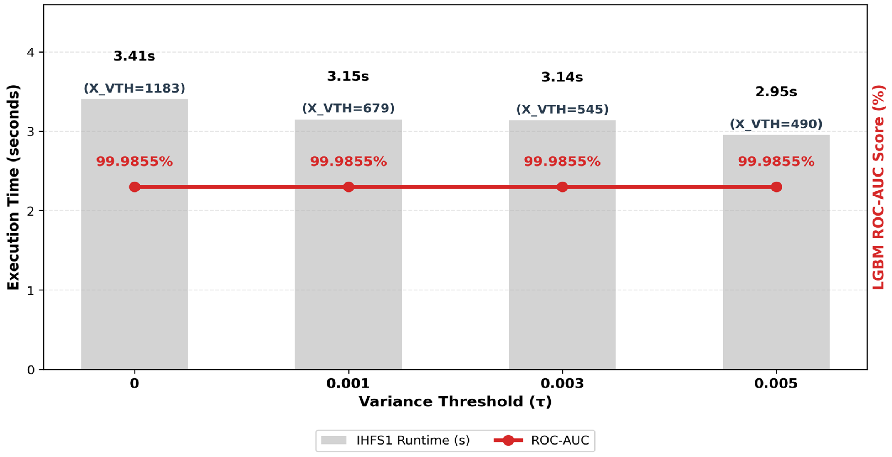
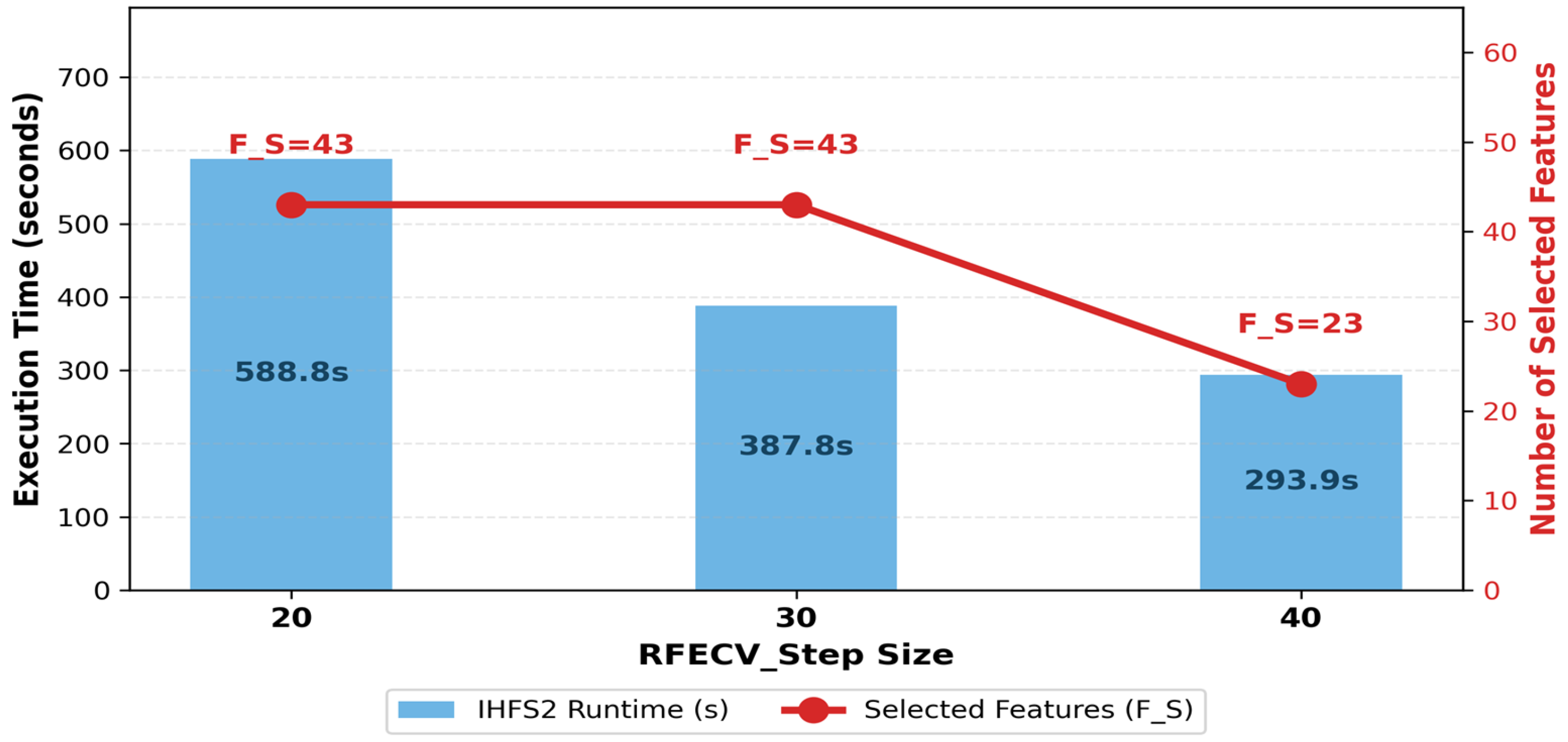
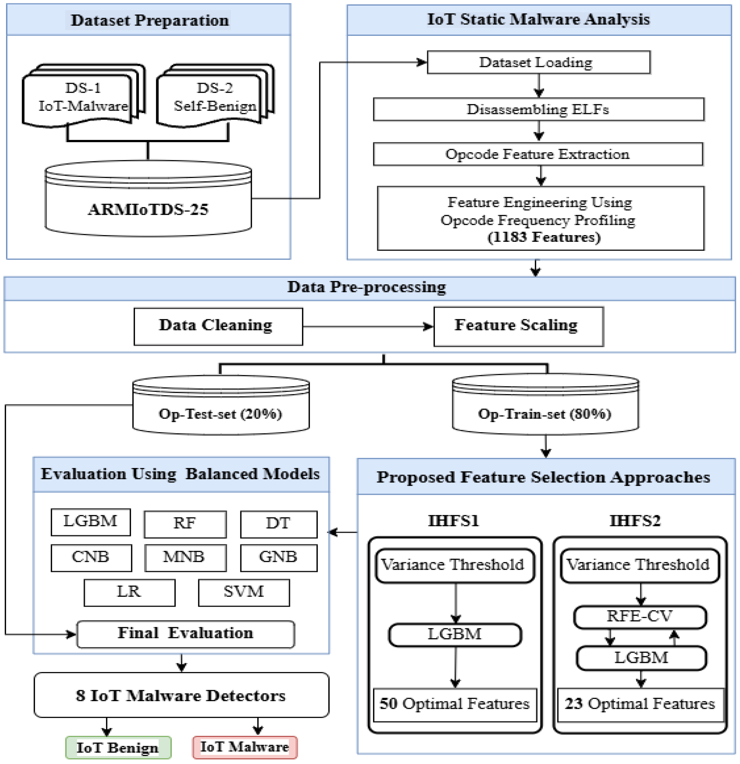
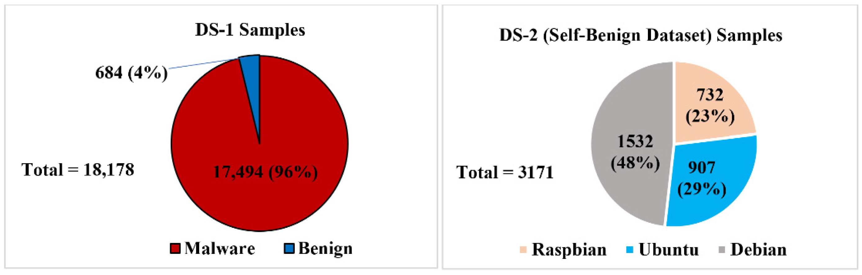


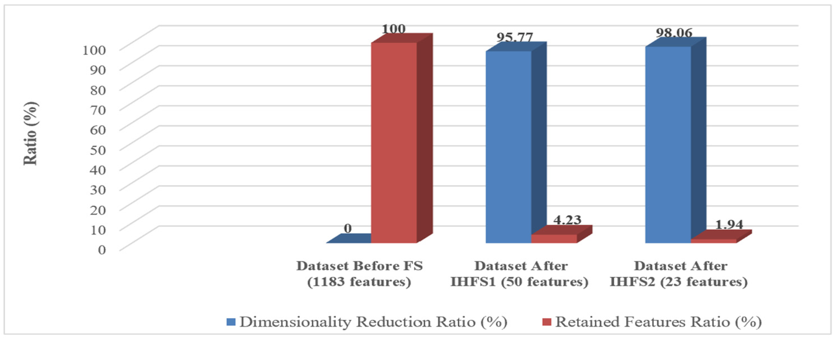


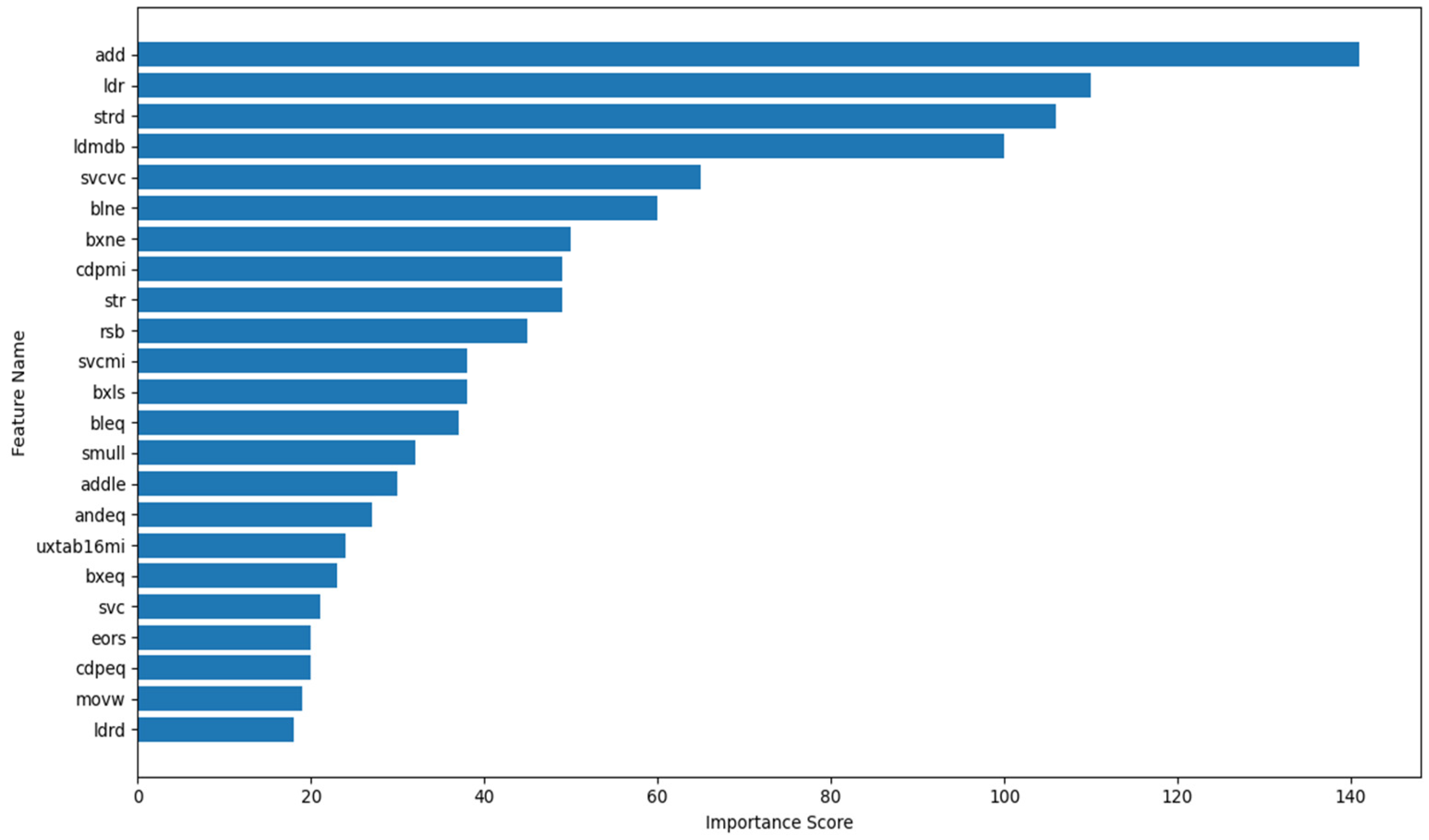
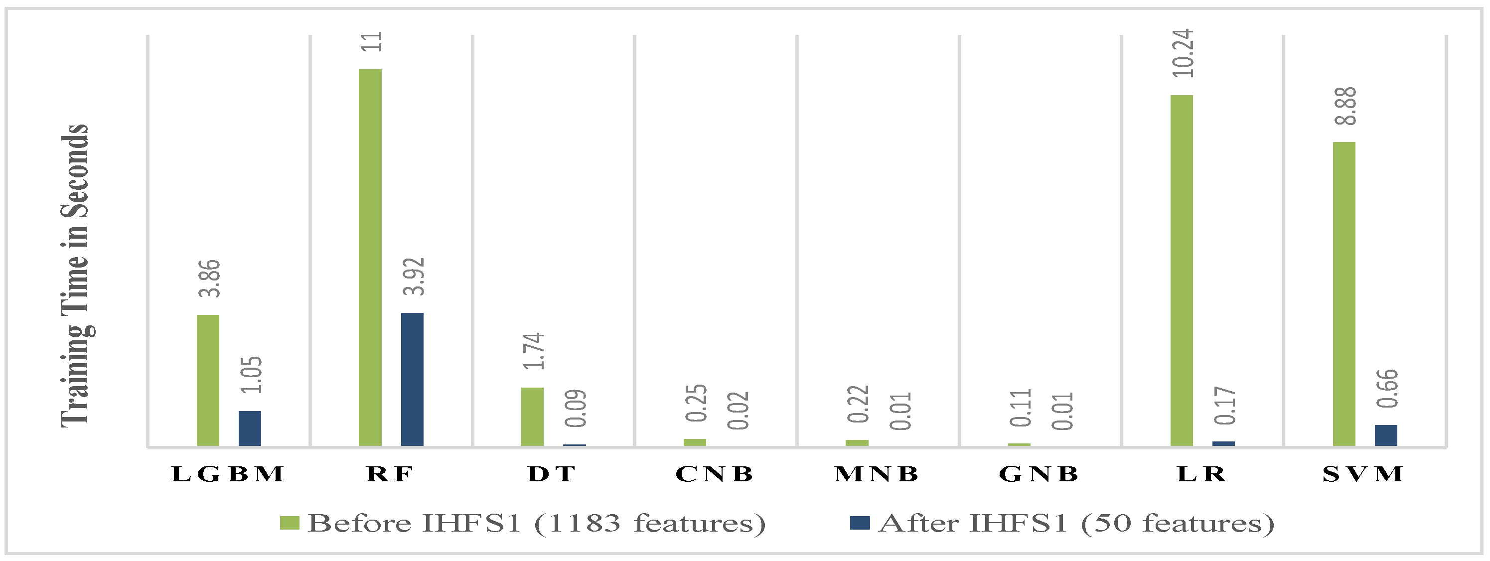
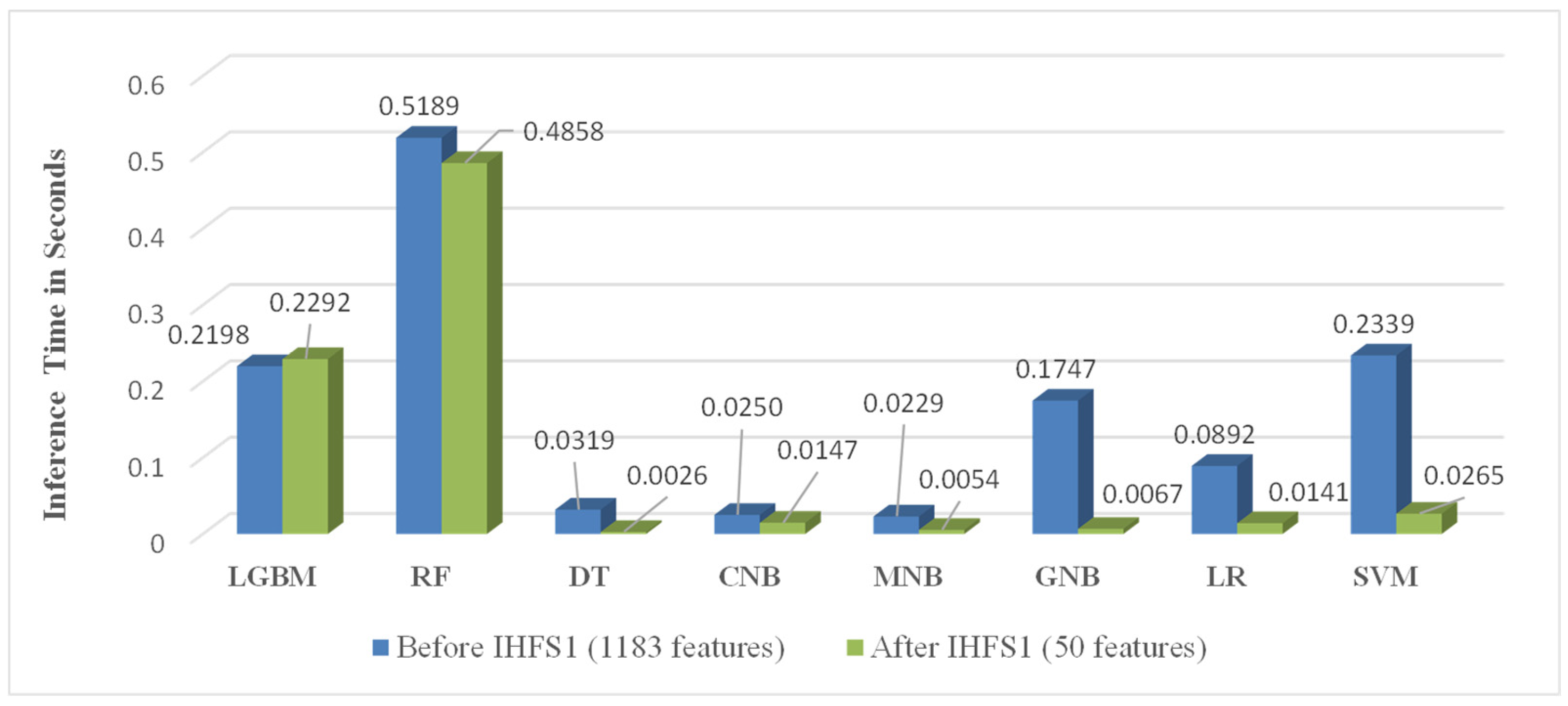


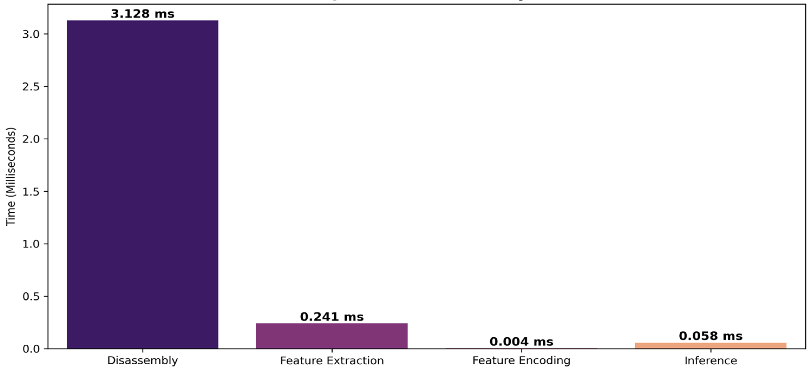
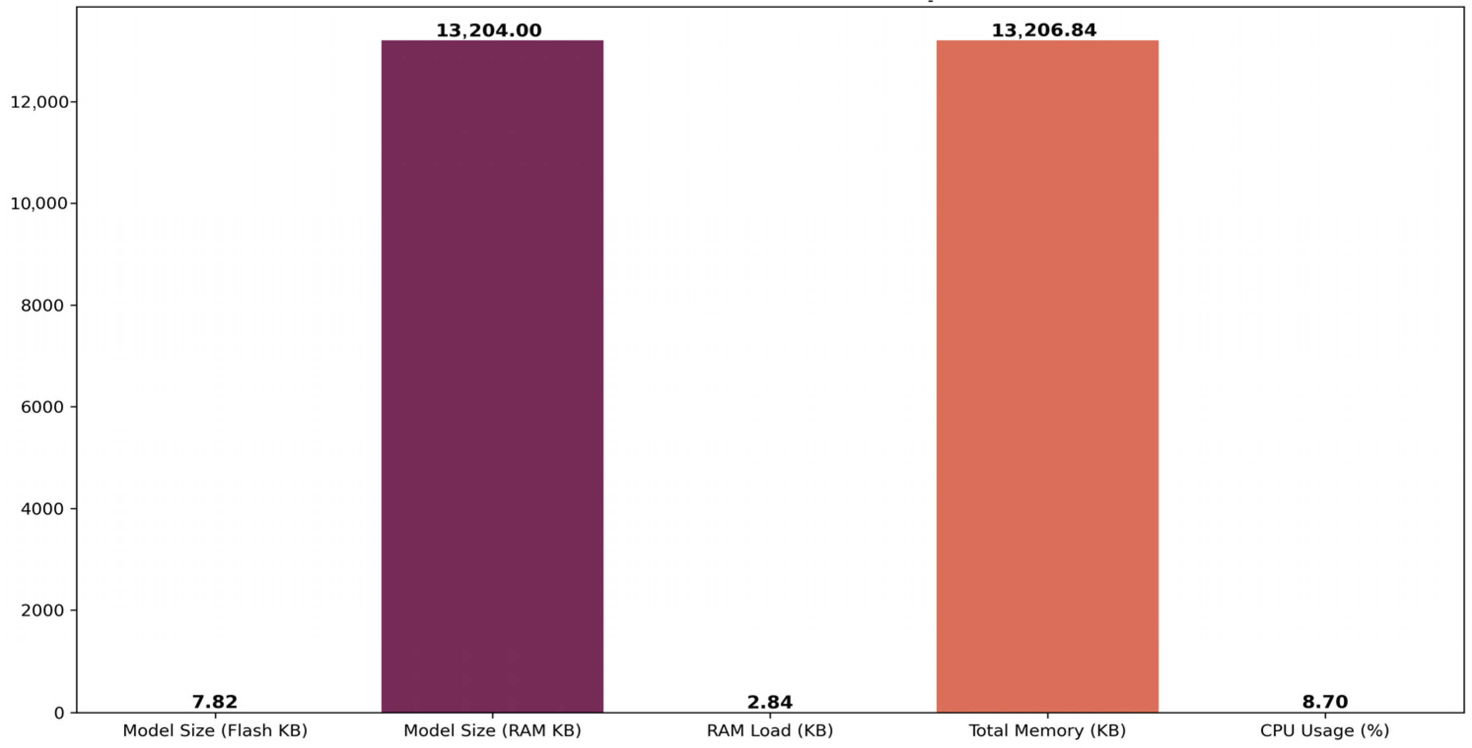

 Filter