
Enhancing Automatic Modulation Recognition for IoT Applications Using Transformers

 , , and
Abstract
1. Introduction
2. Datasets
- RadioML2016.10b [16]:This dataset is composed of ten modulations, including eight digital and two analog modulation types over SNR values ranging from −20 dB to +18 dB, in increments of 2 dB, i.e., . These samples are uniformly distributed across this SNR range. The dataset, which includes a total of 1.2 million samples with a frame size of 128 complex samples, is labeled with both SNR values and modulation types. The dataset is split equally among all considered modulation types. At each SNR value, the dataset contains 60,000 samples, divided equally among the ten modulation types, with 6000 samples for each type. For the channel model, simple multi-path fading with less than five paths was randomly simulated in this dataset. It also includes random channel effects and hardware-specific noises through a variety of models, including sample rate offset, the noise model, center frequency offset, and the fading model. Thermal noise was used to set the desired SNR of each data frame.
- CSPB.ML.2018+ [17]:This dataset is derived from the CSPB.ML.2018 [17] dataset, which aims to solve the known problems and errata [18] with the RadioML2016.10b [16] dataset. CSPB.ML.2018 only provides basic thermal noise as the transmission channel effects. We extended CSPB.ML.2018 by introducing realistic terrain-derived channel effects based on the 3GPP 5G channel model [19]. CSPB.ML.2018+ contains eight different digital modulation modes, totaling 3,584,000 signal samples. Each modulation type has signals with a length of 1024 IQ samples. The channel effects applied include slow and fast multi-path fading, Doppler, and path loss. The transmitter and receiver placements for the 3GPP 5G channel model are randomly selected inside a 6 × 6 km square. The resulting dataset covers an SNR () range of −20 to 40 dB with the majority of SNRs distributed log-normally with dB and dB using as the log conversion method.
3. Transformer Architectures
3.1. TransDirect
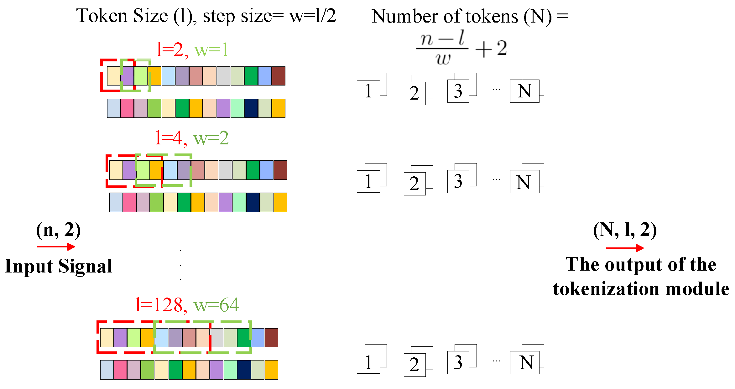
3.2. TransDirect-Overlapping
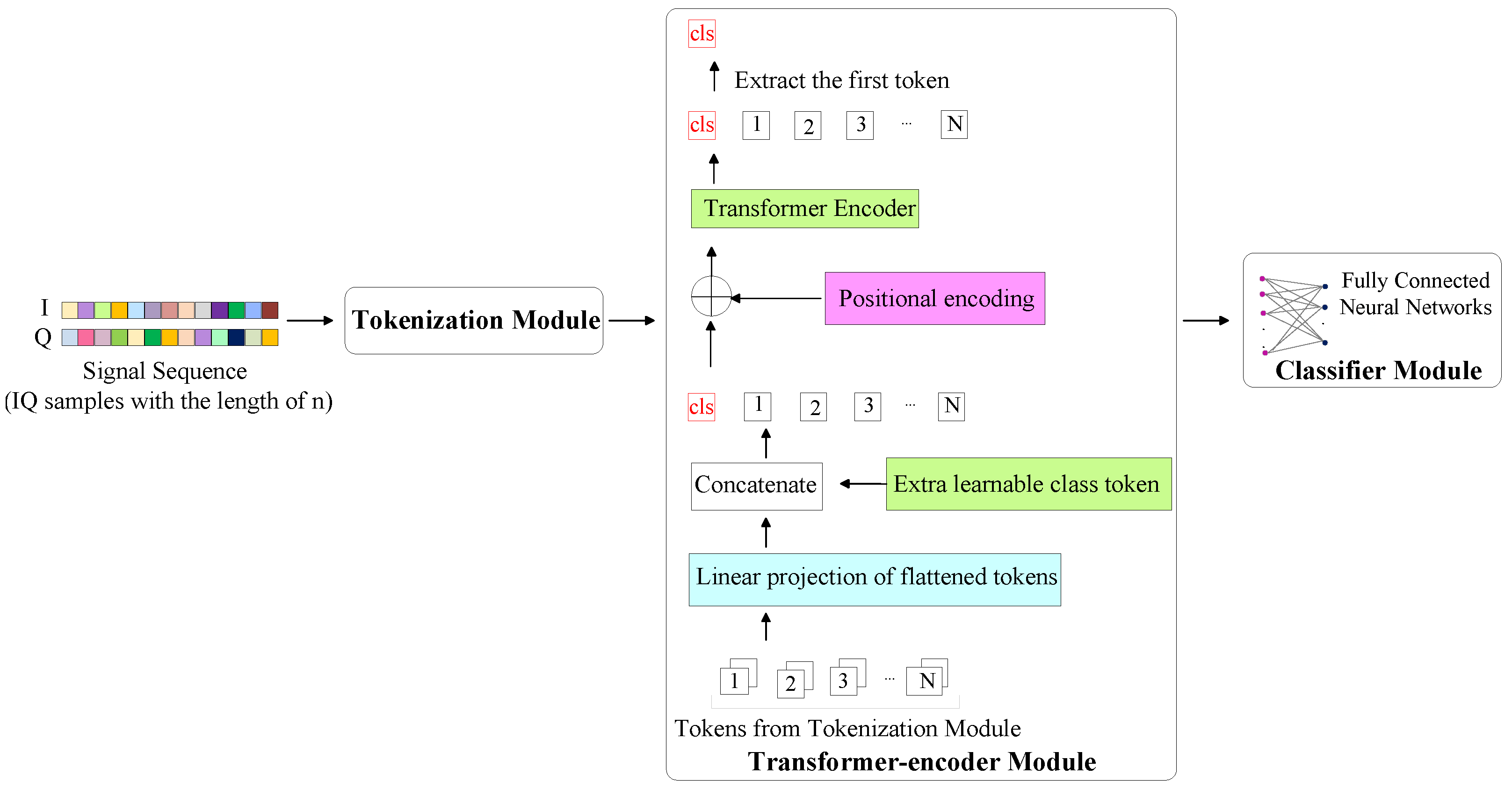
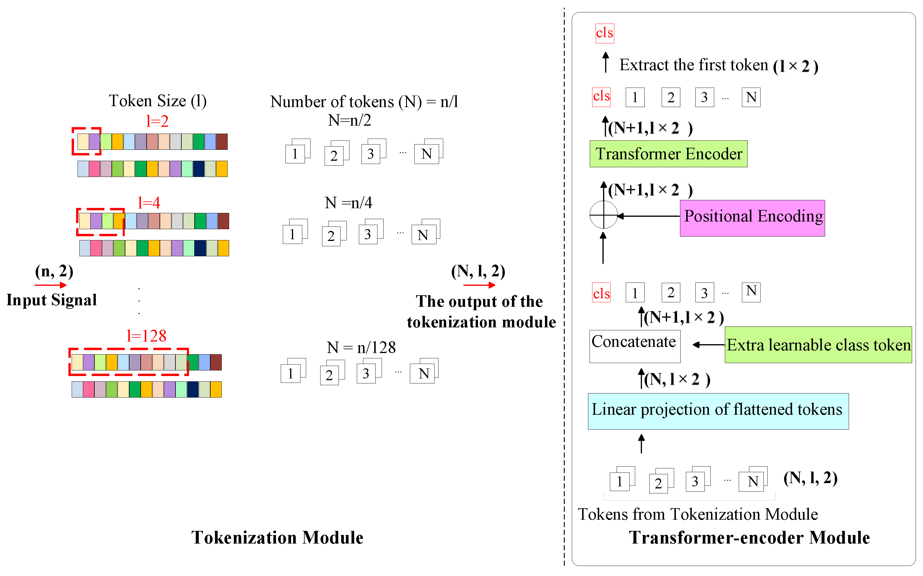
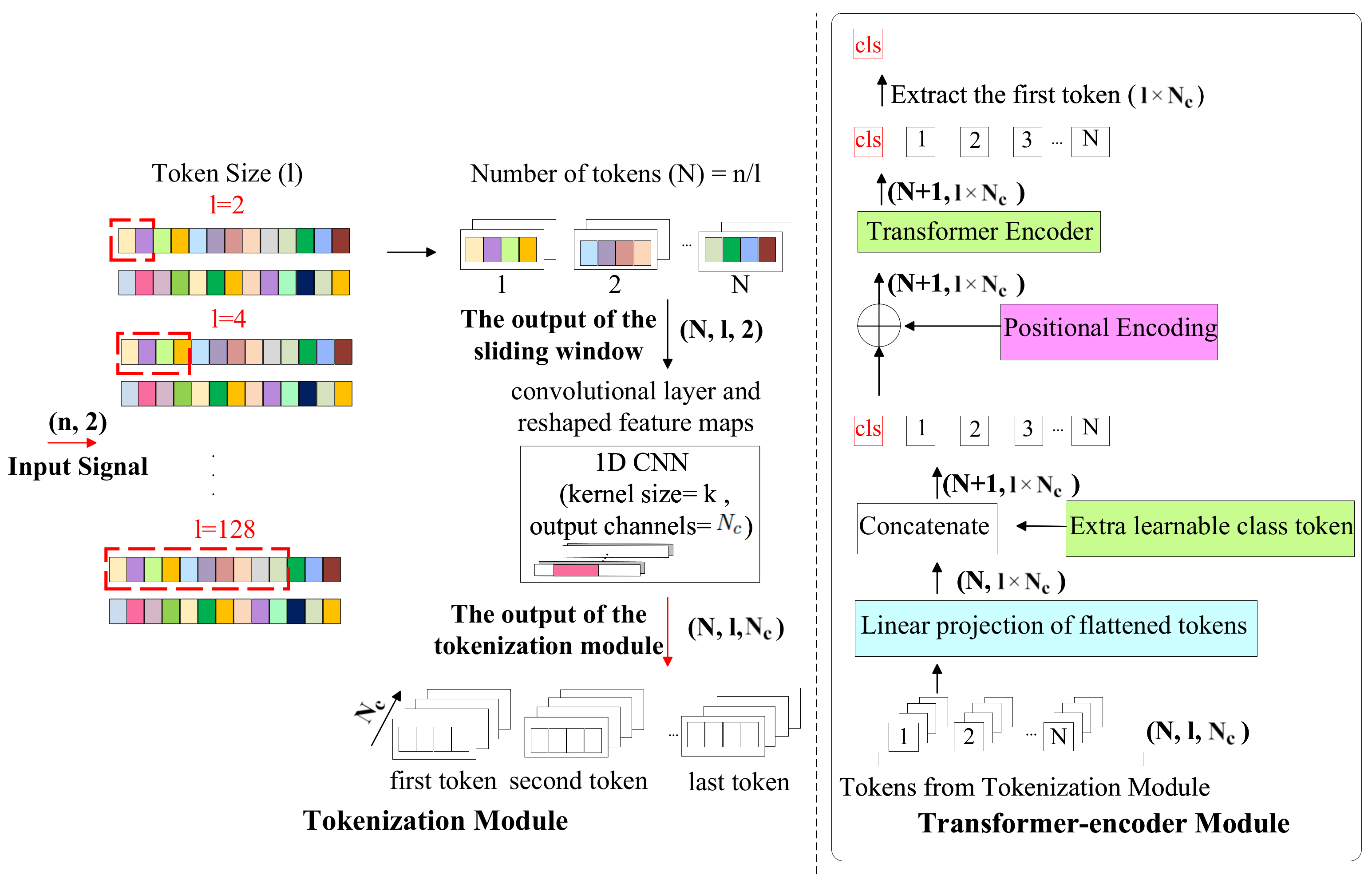
3.3. TransIQ
3.4. TransIQ-Complex
4. Experimental Results and Discussion
4.1. Ablation Study
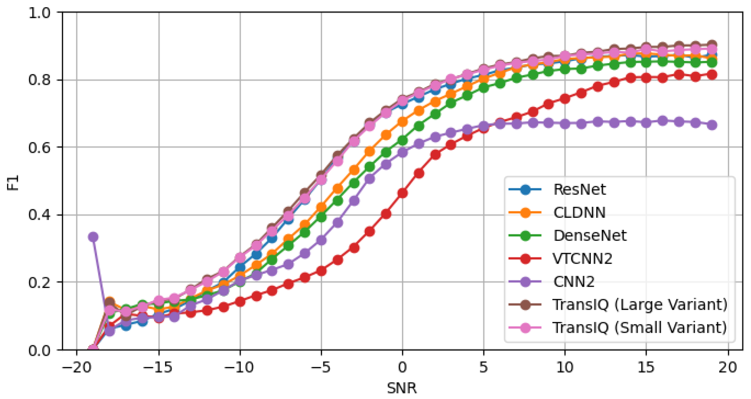
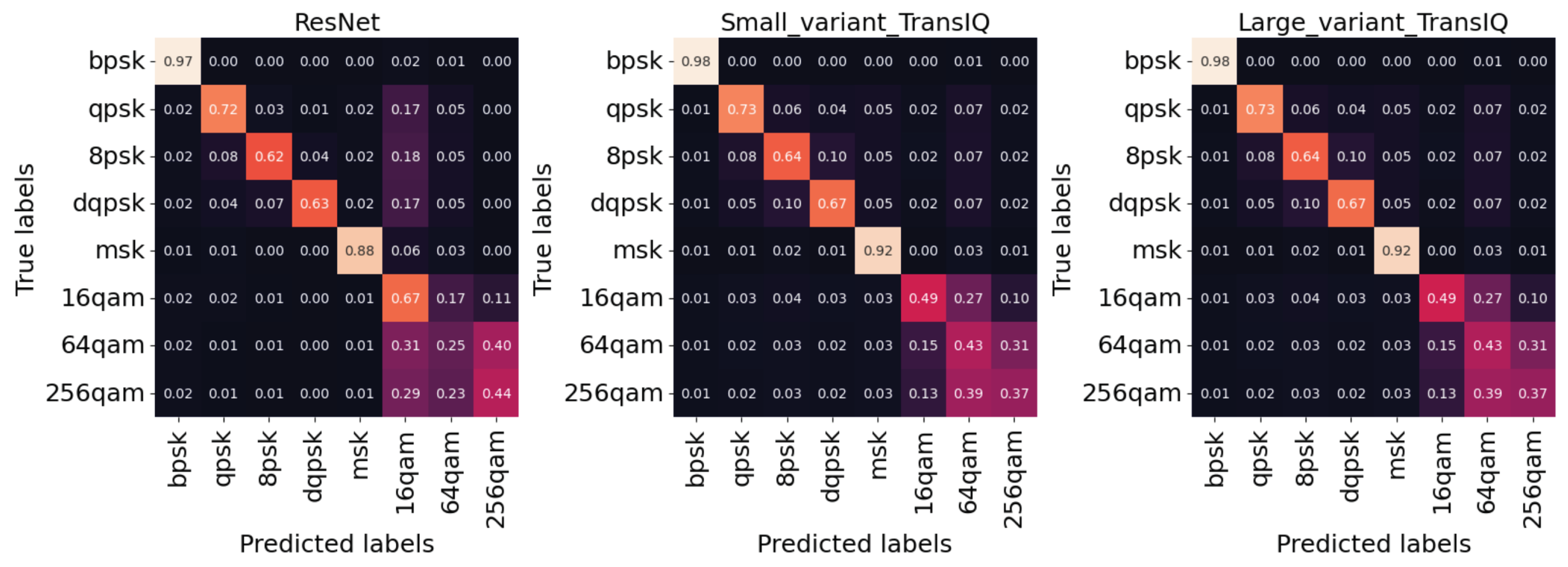
4.2. Comparison with Other Baseline Methods
4.3. Latency and Throughput Metrics
5. Future Investigation
6. Conclusions
Author Contributions
Funding
Data Availability Statement
Conflicts of Interest
Abbreviations
| AMR | automatic modulation recognition |
| IoT | Internet of Things |
| DN | deep learning |
| SNR | signal-to-noise ratio |
| RNNs | recurrent neural networks |
| NLP | natural language processing |
| ViT | vision Transformer |
| CNN | convolutional neural network |
| RF | Radio Frequency |
References
- Zhang, T.; Shuai, C.; Zhou, Y. Deep Learning for Robust Automatic Modulation Recognition Method for IoT Applications. IEEE Access 2020, 8, 117689–117697. [Google Scholar] [CrossRef]
- Zhou, Q.; Zhang, R.; Zhang, F.; Jing, X. An automatic modulation classification network for IoT terminal spectrum monitoring under zero-sample situations. EURASIP J. Wirel. Commun. Netw. 2022, 2022, 25. [Google Scholar] [CrossRef]
- Rashvand, N.; Hosseini, S.; Azarbayjani, M.; Tabkhi, H. Real-Time Bus Arrival Prediction: A Deep Learning Approach for Enhanced Urban Mobility. In Proceedings of the 13th International Conference on Operations Research and Enterprise Systems—ICORES, Rome, Italy, 24–26 February 2024; pp. 123–132. [Google Scholar] [CrossRef]
- Khaleghian, S.; Tran, T.; Cho, J.; Harris, A.; Sartipi, M. Electric Vehicle Identification in Low-Sampling Non-Intrusive Load Monitoring Systems Using Machine Learning. In Proceedings of the 2023 IEEE International Smart Cities Conference (ISC2), Bucharest, Romania, 24–27 September 2023; pp. 1–7. [Google Scholar]
- Vaswani, A.; Shazeer, N.; Parmar, N.; Uszkoreit, J.; Jones, L.; Gomez, A.N.; Kaiser, Ł.; Polosukhin, I. Attention is all you need. Adv. Neural Inf. Process. Syst. 2017, 30. [Google Scholar] [CrossRef]
- Gholami, S.; Leng, T.; Alam, M.N. A federated learning framework for training multi-class OCT classification models. Investig. Ophthalmol. Vis. Sci. 2023, 64, PB005. [Google Scholar]
- O’Shea, T.J.; Roy, T.; Clancy, T.C. Over-the-air deep learning based radio signal classification. IEEE J. Sel. Top. Signal Process. 2018, 12, 168–179. [Google Scholar] [CrossRef]
- Krzyston, J.; Bhattacharjea, R.; Stark, A. High-capacity complex convolutional neural networks for I/Q modulation classification. arXiv 2020, arXiv:2010.10717. [Google Scholar]
- Rajendran, S.; Meert, W.; Giustiniano, D.; Lenders, V.; Pollin, S. Deep learning models for wireless signal classification with distributed low-cost spectrum sensors. IEEE Trans. Cogn. Commun. Netw. 2018, 4, 433–445. [Google Scholar] [CrossRef]
- Ramjee, S.; Ju, S.; Yang, D.; Liu, X.; Gamal, A.E.; Eldar, Y.C. Fast deep learning for automatic modulation classification. arXiv 2019, arXiv:1901.05850. [Google Scholar]
- Hamidi-Rad, S.; Jain, S. Mcformer: A transformer based deep neural network for automatic modulation classification. In Proceedings of the 2021 IEEE Global Communications Conference (GLOBECOM), Madrid, Spain, 7–11 December 2016; pp. 1–6. [Google Scholar]
- Usman, M.; Lee, J.A. AMC-IoT: Automatic modulation classification using efficient convolutional neural networks for low powered IoT devices. In Proceedings of the 2020 International Conference on Information and Communication Technology Convergence (ICTC), Jeju Island, Republic of Korea, 21–23 October 2020; pp. 288–293. [Google Scholar]
- Dosovitskiy, A.; Beyer, L.; Kolesnikov, A.; Weissenborn, D.; Zhai, X.; Unterthiner, T.; Dehghani, M.; Minderer, M.; Heigold, G.; Gelly, S.; et al. An image is worth 16 × 16 words: Transformers for image recognition at scale. arXiv 2020, arXiv:2010.11929. [Google Scholar]
- Rajagopalan, V.; Kunde, V.T.; Valmeekam, C.S.K.; Narayanan, K.; Shakkottai, S.; Kalathil, D.; Chamberland, J.F. Transformers are Efficient In-Context Estimators for Wireless Communication. arXiv 2023, arXiv:2311.00226. [Google Scholar]
- Wang, P.; Cheng, Y.; Dong, B.; Hu, R.; Li, S. WIR-Transformer: Using Transformers for Wireless Interference Recognition. IEEE Wirel. Commun. Lett. 2022, 11, 2472–2476. [Google Scholar] [CrossRef]
- O’shea, T.J.; West, N. Radio machine learning dataset generation with gnu radio. In Proceedings of the GNU Radio Conference, University of Colorado, Boulder, CO, USA, 12–16 September 2016; Volume 1. [Google Scholar]
- Spooner, C.M. Dataset for the Machine-Learning Challenge [CSPB.ML.2018]. Available online: https://cyclostationary.blog/2019/02/15/data-set-for-the-machine-learning-challenge/ (accessed on 1 August 2023).
- All BPSK Signals—Cyclostationary Signal Processing. Available online: https://cyclostationary.blog/2020/04/29/all-bpsk-signals/ (accessed on 1 August 2023).
- 3GPP. Study on Channel Model for Frequencies from 0.5 to 100 GHz, Technical Report (TR) 38.901, version 14.3.0 Release 14, 3rd Generation Partnership Project; 3GPP: Valbonne, France, 2020. [Google Scholar]
- Restuccia, F.; D’Oro, S.; Al-Shawabka, A.; Rendon, B.C.; Ioannidis, S.; Melodia, T. DeepFIR: Addressing the Wireless Channel Action in Physical-Layer Deep Learning. arXiv 2020, arXiv:2005.04226. [Google Scholar]
- Liu, X.; Yang, D.; Gamal, A.E. Deep Neural Network Architectures for Modulation Classification. In Proceedings of the 2017 51st Asilomar Conference on Signals, Systems, and Computers, Pacific Grove, CA, USA, 29 October–1 November 2017; pp. 915–919. [Google Scholar] [CrossRef]
- Tekbıyık, K.; Ekti, A.R.; Görçin, A.; Kurt, G.K.; Keçeci, C. Robust and Fast Automatic Modulation Classification with CNN under Multipath Fading Channels. In Proceedings of the 2020 IEEE 91st Vehicular Technology Conference (VTC2020-Spring), Antwerp, Belgium, 25–28 May 2020; pp. 1–6. [Google Scholar] [CrossRef]
- Hauser, S.C.; Headley, W.C.; Michaels, A.J. Signal detection effects on deep neural networks utilizing raw IQ for modulation classification. In Proceedings of the MILCOM 2017-2017 IEEE Military Communications Conference (MILCOM), Baltimore, MD, USA, 23–25 October 2017; pp. 121–127. [Google Scholar]


| RadioML2016.10b [16] | CSPB.ML.2018+ | |
|---|---|---|
| Number of Modulation Types | 10 (8 digital and 2 analog modulations) | 8 digital modulations |
| Modulation Pool | BPSK, QPSK, 8PSK, QAM16, QAM64, BFSK, CPFSK, PAM4, WBFM, AM-DSB | BPSK, QPSK, 8PSK, DQPSK, MSK, 16-QAM, 64-QAM, 256-QAM |
| Signal Length | 128 | 1024 |
| SNR Range | −20 dB to +18 dB | −19 dB to +40 dB |
| Number of Samples | 1,200,000 | 3,584,000 |
| Sample Distribution across SNR Range | log-uniform distribution | log-normal distribution |
| Channel Effects |
|
|
| Methods | Tokenization | F1 Score | Number of Parameters |
|---|---|---|---|
| TransDirect | 8 samples | 53.15 | 17.2 K |
| 16 samples | 56.29 | 44.1 K | |
| 32 samples | 56.20 | 128 K | |
| 64 samples | 52.24 | 420 K | |
| TransDirect-Overlapping | 8 samples | 53.98 | 17.2 K |
| 16 samples | 59.43 | 44.1 K | |
| 32 samples | 60.08 | 128 K | |
| 64 samples | 57.67 | 420 K | |
| TransIQ | 8 samples with 8 output channels (head = 2, layer = 4) | 63.69 | 128 K |
| 8 samples with 16 output channels (head = 2, layer = 4) | 63.25 | 420 K | |
| 16 samples with 8 output channels (head = 2, layer = 4) | 63.72 | 420 K | |
| 32 samples with 8 output channels (head = 2, layer = 4) | 62.68 | 1.5 M | |
| 8 samples with 8 output channels (head = 4, layer = 8) | 65.80 | 229 K | |
| 8 samples with 8 output channels (head = 2, layer = 6) | 65.39 | 179 K | |
| TransIQ-Complex | 8 samples with 8 output channels (head = 2, layer = 4) | 61.19 | 420 K |
| 16 samples with 8 output channels (head = 2, layer = 4) | 62.79 | 1.5 M | |
| 32 samples with 8 output channels (head = 2, layer = 4) | 59.33 | 5.6 M |
| Methods | F1 Score | Number of Parameters |
|---|---|---|
| DenseNet [21] | 56.93 | 3.3 M |
| CLDNN [21] | 61.14 | 1.3 M |
| VTCNN2 [23] | 61.53 | 5.5 M |
| CNN2 [22] | 60.94 | 1 M |
| ResNet [7] | 64.62 | 107 K |
| Mcformer [11] | 65.03 | - |
| TransIQ (large variant) | 65.75 | 229 K |
| TransIQ (small variant) | 65.61 | 179 K |
| Methods | F1 Score | Number of Parameters |
|---|---|---|
| DenseNet [21] | 57.87 | 21.6 M |
| CLDNN [21] | 61.26 | 7.1 M |
| VTCNN2 [23] | 47.29 | 42.2 M |
| CNN2 [22] | 52.57 | 3.8 M |
| ResNet [7] | 65.48 | 164 K |
| TransIQ (large variant) | 65.80 | 229 K |
| TransIQ (small variant) | 65.39 | 179 K |
| Models | Latency (ms/Sample) | Throughput (Sample/s) |
|---|---|---|
| TransIQ (small variant) | 3.36 | 297.61 |
| TransIQ (large variant) | 5.93 | 168.63 |
Disclaimer/Publisher’s Note: The statements, opinions and data contained in all publications are solely those of the individual author(s) and contributor(s) and not of MDPI and/or the editor(s). MDPI and/or the editor(s) disclaim responsibility for any injury to people or property resulting from any ideas, methods, instructions or products referred to in the content. |
© 2024 by the authors. Licensee MDPI, Basel, Switzerland. This article is an open access article distributed under the terms and conditions of the Creative Commons Attribution (CC BY) license (https://creativecommons.org/licenses/by/4.0/).
Share and Cite
Rashvand, N.; Witham, K.; Maldonado, G.; Katariya, V.; Marer Prabhu, N.; Schirner, G.; Tabkhi, H. Enhancing Automatic Modulation Recognition for IoT Applications Using Transformers. IoT 2024, 5, 212-226. https://doi.org/10.3390/iot5020011
Rashvand N, Witham K, Maldonado G, Katariya V, Marer Prabhu N, Schirner G, Tabkhi H. Enhancing Automatic Modulation Recognition for IoT Applications Using Transformers. IoT. 2024; 5(2):212-226. https://doi.org/10.3390/iot5020011
Chicago/Turabian StyleRashvand, Narges, Kenneth Witham, Gabriel Maldonado, Vinit Katariya, Nishanth Marer Prabhu, Gunar Schirner, and Hamed Tabkhi. 2024. "Enhancing Automatic Modulation Recognition for IoT Applications Using Transformers" IoT 5, no. 2: 212-226. https://doi.org/10.3390/iot5020011
APA StyleRashvand, N., Witham, K., Maldonado, G., Katariya, V., Marer Prabhu, N., Schirner, G., & Tabkhi, H. (2024). Enhancing Automatic Modulation Recognition for IoT Applications Using Transformers. IoT, 5(2), 212-226. https://doi.org/10.3390/iot5020011