Measuring α-FPUT Cores and Tails

Abstract

Almost 70 years ago, the Fermi–Pasta–Ulam–Tsingou (FPUT) paradox was formulated in, observed in, and reported using normal modes of a nonlinear, one-dimensional, non-integrable string. Let us recap the paradox. One normal mode is excited, which drives three or four more normal modes in the core. Then, that is it for quite a long time. So why are many normal modes staying weakly excited in the tail? Furthermore, how many? A quantitative, analytical answer to the latter question is given here using resonances and secular avalanches A comparison with the previous numerical data is made and extremely good agreement is found.

1. Introduction

In 1955, Fermi, Pasta, Ulam and Tsingou published their celebrated report on the thermalization of weakly nonlinear strings [1], bringing forth a fundamental physical and mathematical problem of energy equipartition and ergodicity. The study was reportedly performed by Enrico Fermi, John Pasta, Stanislav Ulam, and Mary Tsingou, and the internal Los Alamos report was written and authored by Fermi, Pasta and Ulam [1]. A series of numerical simulations showed that energy, initially placed in a low-frequency normal mode of the linear problem with a frequency ${\omega }_q$ and a corresponding wave number q, stayed almost completely locked within a few neighbor low-frequency modes in the presence of nonlinear mode–mode interactions, instead of being distributed among all modes of the system. Moreover, the recurrence of energy to the originally excited mode was observed after a long simulation time. It has been known since as the Fermi–Pasta–Ulam–Tsingou (FPUT) problem, paradox, and discovery [2,3,4,5].

A number of studies have focused on the explanation of recurrences. Zabusky and Kruskal pioneered the pathway of integrable approximations and soliton counting in real space [6,7,8]. To connect to the limit of weak nonlinear dynamics, Ford and Jackson followed the path of resonances in normal mode space [9,10,11]. Tuck and Menzel (née Tsingou) studied in detail the fate of recurrences for longer times. To their surprise, they observed super-recurrences, i.e., beatings of the recurrence amplitudes [12]. Sholl and Henry searched for scaling relations from recurrence time computations [13]. Lin, Goedde, and Lichter arrived at more detailed scaling relations for the recurrence times, and in addition also produced intriguing numerical data for the dependence of the number of excited modes of the energy [14]. The framework of periodic orbits in dynamical systems was used to rigorously prove the existence of exact time-periodic orbits, coined q-breathers, which are nonlinearity-induced deformed normal-mode periodic orbits of the linear limit [15,16]. FPUT trajectories correspond to perturbed q-breather solutions. An advanced perturbation analysis in mode space which uses secular avalanches was derived by Ponno et al. [17], which arrived at an approximate estimate of the excited mode number in the FPUT experiment. Recently, Pace and Campbell arrived at an elegant theoretical quantitative explanation of super-recurrences [18]. What remains, then, is to quantitatively explain the numerical observations on the excited mode number by Lin et al. [14] which is what is done below.

2. The $\mathbf{\alpha }$-FPUT Chain

FPUT-studied models have cubic ($\alpha$-FPUT) and quartic ($\beta$-FPUT) nonlinearities in the Hamiltonian potential energy, and the $\alpha$-FPUT case is considered here. The Hamiltonian of the $\alpha$-FPUT lattice for N particles is given by

$$H_{\alpha }(\mathbf{q},\mathbf{p})=\sum _{n=1}^N\frac{p_n^2}{2}+\sum _{n=0}^N\frac{1}{2}{(q_{n+1}-q_n)}^2+\frac{\alpha }{3}{(q_{n+1}-q_n)}^3.$$

(1)

Fixed boundary conditions, $q_0=q_{N+1}=0$ and $p_0=p_{N+1}=0$ are used, where $q_n\left(t\right)$ and $p_n\left(t\right)$ are canonical coordinates and momenta, respectively.

The normal-mode representation is introduced via a canonical Fourier transform,

$$\left[\begin{array}{c}{q}_n\\ p_n\end{array}\right]=\sqrt{\frac{2}{N+1}}\sum _{k=1}^N\left[\begin{array}{c}{Q}_k\\ P_k\end{array}\right]sin\left(\frac{nk\pi }{N+1}\right),$$

(2)

which diagonalizes the harmonic oscillator Hamiltonian part. Rewriting Equation (1) in these normal-mode coordinates ($\mathbf{Q},\mathbf{P}$) yields:

$$H_{\alpha }(\mathbf{Q},\mathbf{P})=\sum _{k=1}^N\frac{P_k^2+{\omega }_k^2{Q}_k^2}{2}+\frac{\alpha }{3}\sum _{k,j,l=1}^N{A}_{k,j,l}{Q}_k{Q}_j{Q}_l,$$

(3)

where the normal mode frequencies are

$${\omega }_k=2sin\left(\frac{k\pi }{2(N+1)}\right),$$

(4)

and the normal mode energies are defined as

$$E_k=\frac{P_k^2+{\omega }_k^2{Q}_k^2}{2}.$$

(5)

Note that these normal mode energies are conserved quantities for $\alpha =0$, but cease to be preserved for the nonlinear case. The coupling constants $A_{k,j,l}$ are given by [16]

$$A_{k,j,l}=\frac{{\omega }_k{\omega }_j{\omega }_l}{\sqrt{2(N+1)}}\sum _{\pm }\left({\delta }_{k,\pm j\pm l}-{\delta }_{k\pm j\pm l,2(N+1)}\right).$$

(6)

Here, the sums ${\sum }_{\pm }$ are overall combinations of plus and minus signs among the ± symbols, and ${\delta }_{j,l}$ is the Kronecker delta function.

One can rescale the normal-mode coordinate and momentum [19] pairs in Equation (3) by $(\mathbf{Q},\mathbf{P})\to (\mathbf{Q}/\alpha ,\mathbf{P}/\alpha )$. If E represents the total energy in the system, this leads to

$$H_{\alpha =1}(\mathbf{Q},\mathbf{P})={\alpha }^{2}E,$$

(7)

which allows one to investigate results as functions of the combined parameter, $E{\alpha }^2$, rather than using the separate parameters E and $\alpha$.

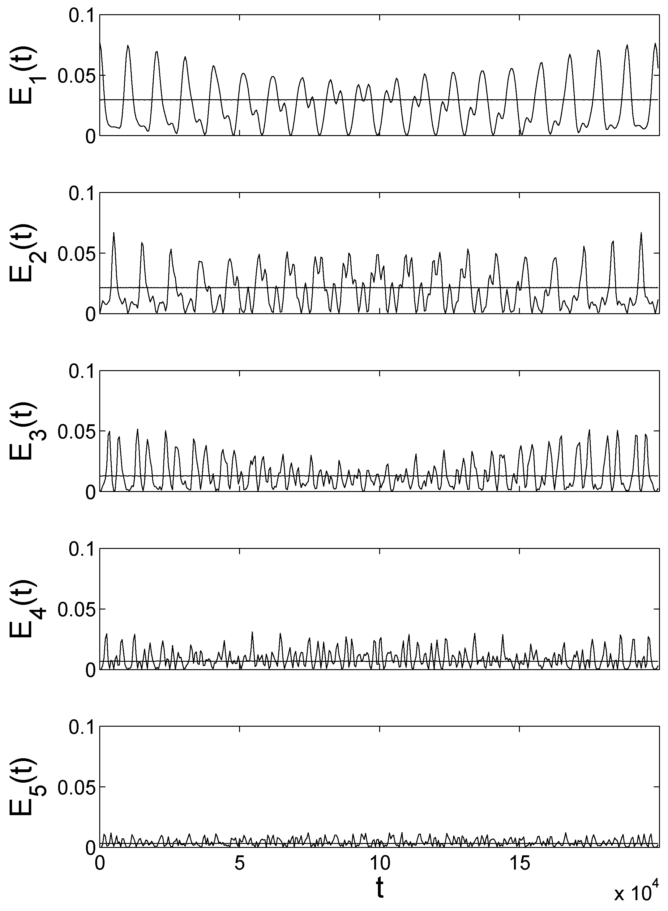
Let us show the evolution of the original $\alpha$-FPUT trajectory for $\alpha =0.25$, $N=32$ and energy $E=0.077$ placed initially into the mode with $k_0=1$. (All variables in this paper are considered dimensionless.) In Figure 1, the time dependence of the mode energies $E_k\left(t\right)$ is plotted for the first five modes of the data from [16].

The period of the slowest ($k_0=1$) harmonic mode is $T_1=2\pi /{\omega }_1\approx 66.02$. One observes slow processes of the redistribution of mode energies, with recurrence time amounting to $T_{\mathrm{R}}\approx 10530$. One can also observe even slower modulations of recurrence amplitudes on time scales of the order of ${10}^5$, which are the celebrated super-recurrences with $T_{\mathrm{SR}}\approx 2\times {10}^6$ [12,18]. The localization in q-space is also well observed, with the maximum of $E_5$ being eight times smaller than that of $E_1$. The number of strongly participating modes can be therefore estimated to be around three or four. The almost straight horizontal lines indicate the weak time dependence of the linear mode energies on the corresponding exact time-periodic q-breather solutions from [16].

3. Mode Coupling Approach

The equations of motion for the normal mode amplitudes follow from Equations (1)–(6) and read:

$${\ddot{Q}}_k+{\omega }_k^2{Q}_k=-\alpha \sum _{l,m=1}^N{A}_{k,l,m}{Q}_l{Q}_m,$$

(8)

where the dots stay for time derivative.

The system of Equation (8) describes a network of oscillators with different eigenfrequencies. These oscillators interact with each other via nonlinear interaction terms. The interaction network is long-ranged in k-space. To be more specific, each normal-mode oscillator is interacting with a set of other doublets of oscillators. The total number of multiplets one normal-mode oscillator is connected to is proportional to $N^2$. The number N is the total number of oscillators (particles), or, more generally, the volume of the system. The coupling constants $A_{k,l,m}$ depend on the oscillator frequencies; see Equation (6). Still, their values do not decay exponentially fast, with some growing distance between oscillators (after introducing a proper metric). Therefore, essentially all oscillators interact with all others. This is what is meant by “long range”.

If there is long-range interaction in mode space, why do modes not quickly excite other modes and thermalize? The reason is that the interaction is nonlinear. Indeed, with linear interactions, exciting one mode will inevitably excite other modes in some proportion to the coupling coefficient amplitudes. However, with nonlinear couplings, things are more complicate as shown below. Actually, it is insightful to recall the seemingly simple problem of the periodic motion of one oscillator in an anharmonic potential,

$$\ddot{x}=-x-\alpha x^2-\beta x^3,$$

(9)

where x is the space coordinate.

The bounded motion at energy E yields a solution which is periodic with some period, $T\left(E\right)=2\pi /\mathrm{\Omega }$ (with $\mathrm{\Omega }$ denoting the frequency), and can be represented by a Fourier series

$$x\left(t\right)=\sum _k{A}_k{\mathrm{e}}^{ik\mathrm{\Omega }t},$$

(10)

which leads to algebraic equations for the Fourier coefficients,

$$A_k=k^2{\Omega }^2{A}_k-\alpha \sum _{k_1}{A}_{k_1}{A}_{k-k_1}-\beta \sum _{k_1,k_2}{A}_{k_1}{A}_{k_2}{A}_{k-k_1-k_2}.$$

(11)

Let us note that Equation (11) has similar properties as compared to Equation (8)—the coupling between the Fourier coefficients is nonlinear but long ranged. Yet, it is known that the bounded solutions (10) to (9) are analytic functions $x\left(t\right)$, and thus the Fourier series coefficients $A_k$ converge exponentially fast with k [20].

3.1. Complex Mode Variables

Ponno et al. [17] attempted to obtain analytical expressions for the mode dynamics of the $\alpha$-FPUT model at times shorter than, or at best of the order of the time of first recurrence. Following their approach, let us perform a change from real to complex variables:

$$u_k\equiv \frac{{\omega }_k{Q}_k+i{P}_k}{\sqrt{2E}},{\left|u_k\left(t\right)\right|}^2=\frac{E_k\left(t\right)}{E}=e_k\left(t\right),$$

(12)

The $\alpha$-FPUT Hamiltonian now reads:

$$\mathcal{H}(u,u^{*})=\underset{{\mathcal{H}}_2}{\underbrace{\sum _{k=1}^{N-1}{\left|u_k\right|}^2}}+\underset{{\mathcal{H}}_3}{\underbrace{\frac{\mu }{12}\sum _{k_1,k_2,k_3=1}^{N-1}{\Delta }_{k_1,k_2,k_3}\prod _{j=1}^3(u_{k_j}+u_{k_j}^{*})}},$$

(13)

where

$${\Delta }_{k_1,k_2,k_3}\equiv {\delta }_{k_1+k_2,k_3}+{\delta }_{k_2+k_3,k_1}+{\delta }_{k_3+k_1,k_2}-{\delta }_{k_1+k_2+k_3,2N},$$

(14)

and

$$\mu \equiv \alpha \sqrt{\frac{E}{N}}.$$

(15)

The quadratic, ${\mathcal{H}}_2$, and cubic, ${\mathcal{H}}_3$, parts of the Hamiltonian are indicated in Equation (13). The equations of motion then read:

$${\dot{u}}_k=-i{\omega }_k\left[u_k+\frac{\mu }{4}\sum _{p,q=1}^{N-1}{\Delta }_{k,p,q}(u_p+u_p^{*})(u_q+u_q^{*})\right].$$

(16)

The FPUT initial condition turns to

$$u_k\left(0\right)={\delta }_{k,1}.$$

(17)

3.2. Resonances

With the FPUT initial condition of exciting mode $k=1$, and a small value of $\mu$ in Equation (15), the first mode starts evolving in an almost periodic fashion with a frequency almost equal to ${\omega }_1$. Assuming $u_k=e^{-i{\omega }_{1}t}{\delta }_{k,1}$ as a solution to zero order in $\mu$, and inserting this into the righ-hand side (r.h.s.) of Equation (16) leaves us with

$${\dot{u}}_2+i{\omega }_2{u}_2=-i\mu {\omega }_2{cos}^2{\omega }_{1}t\equiv -i\frac{\mu {\omega }_2}{2}(1+cos2{\omega }_{1}t).$$

(18)

Thus, mode $k=2$ is driven by a periodic force with frequency $2{\omega }_1$. This is as close to resonance as ${\omega }_2-2{\omega }_1$ is close to zero, and its smallness is to be compared with the drive amplitude ∼$\mu {\omega }_2$. Assuming $\pi /\left(2\right(N+1\left)\right)\ll 1$, which is correct for $N=32$, let us expand the dispersion relation: ${\omega }_k=2sin\left(\frac{k\pi }{2(N+1)}\right)\approx 2\left(\frac{\pi k}{2(N+1)}-\frac{{\pi }^3{k}^3}{48{(N+1)}^3}\right)$. Then:

$${\Delta }_2\equiv |{\omega }_2-2{\omega }_1|\approx \frac{{\pi }^3}{4{(N+1)}^3}.$$

(19)

Stripping Equation (18) off its nonresonant terms (whose contribution to the solution is reduced by a factor of ${\Delta }_2/{\omega }_{1,2}\sim 1/N^2$), one is left with

$${\dot{u}}_2+i{\omega }_2{u}_2\approx -i\frac{\mu {\omega }_2}{4}exp(-2i{\omega }_{1}t).$$

(20)

The solution to Equation (20) reads:

$$u_2\left(t\right)=\frac{\mu {\omega }_2}{4{\Delta }_2}{\mathrm{e}}^{-i{\omega }_{2}t}\left[{\mathrm{e}}^{i{\Delta }_{2}t}-1\right].$$

(21)

As long as $u_2\left(t\right)\ll 1$, the above approach is valid. The border of its validity is reached when the energy E takes the critical value $E_2^{\mathrm{sa}}$, at which mode $k=2$ is involved in a secular avalanche [17]:

$$\frac{\mu {\omega }_2}{4{\Delta }_2}=1\to E_2^{\mathrm{sa}}=\frac{{\pi }^4}{36{\alpha }^2{N}^3}.$$

(22)

For energies $E\ll E_2^{\mathrm{sa}}$, the small frequency ${\Delta }_2$ leads to a slow modulation in the r.h.s. of Equation (21), which results in a corresponding slow modulation of the energy stored in mode $k=1$ due to energy conservation. Then, the corresponding zero order (or perturbative) recurrence time estimate is:

$$T_{\mathrm{R}}^{\left(0\right)}\equiv \frac{2\pi }{{\Delta }_2}=\frac{8}{{\pi }^2}{N}^3,E\ll E_2^{\mathrm{sa}}.$$

(23)

This coincides with earlier results by Sholl and Henry [13] ( see also Lin et al. [14]), and the relevant resonance was already worked out in Ford’s paper [9].

Let us calculate some numbers. Figure 1 in Ref. [14] uses parameters $E=2.2$, $\alpha =0.1$, and $N=32$. On one side, it follows $T_{\mathrm{R}}^{\left(0\right)}$ = 26,560, but due to the large energy, it also follows $E\gg E_2^{\mathrm{sa}}=0.0083$, implying that the recurrence time concept is invalid since perturbation theory is inapplicable. Still, the measured $T_{\mathrm{R}}=6400$ is orders of magnitude larger than the typical mode period, $T_1$, and only a factor of four smaller than the perturbation theory estimate. The original FPUT trajectory was investigated in Figure 1 of Ref. [16], with parameters $E=0.077$, $\alpha =0.25$ and $N=32$, and shown here in Figure 1. Again, $E\gg E_2^{\mathrm{sa}}=0.0013$. The measured recurrence time $T_{\mathrm{R}}$ = 10,500 is smaller than the perturbation result $T_{\mathrm{R}}^{\left(0\right)}$, but still orders of magnitude larger than the mode period $T_1$. Part of the FPUT surprise must have been that even for $E\gg E_2^{\mathrm{sa}}$, recurrence times still stayed large and reasonably close to their perturbation theory estimates, and a fast approach to equipartition was missing.

4. The Number of Excited Modes

For $E\gg E_2^{\mathrm{sa}}$, one concludes that the FPUT trajectory is resonant. Mode $k=2$ will be resonantly pumped up by mode $k=1$ until mode $k=1$ is depleted. It is needless to state that the process continues into higher modes, showing a complex resonant avalanche, as studied in detail in Ref. [17]. Furthermore, this is what FPUT observed, since they evidently chose the proper parameters to ensure that the system is in the nonperturbative regime of a resonant avalanche, which one enters for energies $E\ge E_2^{\mathrm{sa}}$.

Why is the secular avalanche stopping and not continuing to flood all the modes? According to Ref. [17], this is simply because the modes in the mode packet can be separated into core modes and tail modes. Core modes are strongly and resonantly interacting with each other. Tail modes fail to be resonantly pumped as they are tuned out of resonance due to the nonlinear dispersion relation. The boundary-separating core and tail modes are functions of the energy. For $E\ll E_2^{\mathrm{sa}}$, all modes are tail modes except for the one core mode initially excited.

To see that the above approach is extended to higher orders of perturbation theory; see Ref. [17] for details. Mode $k=2$ is driven by mode $k=1$ through the resonant term $u_1^2$. Mode $k=3$ is driven by the resonant term $u_1{u}_2$, and so on. One arrives at

$${\dot{u}}_k+i{\omega }_k{u}_k\approx -i\frac{\mu {\omega }_k}{4}{\mathrm{e}}^{-ik{\omega }_{1}t}.$$

(24)

The relevant resonances are ${\Delta }_k=|k{\omega }_1-{\omega }_k|$, and lead to

$$u_k\left(t\right)\approx \frac{\mu {\omega }_k}{4{\Delta }_k}{\mathrm{e}}^{-i{\omega }_{k}t}\left[{\mathrm{e}}^{i{\Delta }_{k}t}-1\right].$$

(25)

The critical energy $E_k^{\mathrm{sa}}$, above which mode k becomes part of the core and the secular avalanche, then reads:

$$\frac{\mu {\omega }_k}{4{\Delta }_k}=1\to E_k^{\mathrm{sa}}=\frac{2{\pi }^4{(k^2-1)}^2}{{24}^2{\alpha }^2{N}^3}.$$

(26)

Since $E_k^{\mathrm{sa}}\sim k^4$, it follows that for some reasonably small value of $k\equiv k_c$, the corresponding mode will be out of resonance:

$$k_c=\sqrt{1+\frac{6}{{\pi }^2}\mu N^2}.$$

(27)

This agrees very well with the detailed derivations in Ref. [17], which culminate in a rough scaling estimate $k_c\approx \sqrt{\mu }N$ for large $k_c$ and large N. At the same time, Equation (27) is accurate for small values of $k_c$, which is the case for, e.g., the original FPUT trajectory (see precise numbers just below). This can happen despite a large value of $N\gg 1$ since other relevant (small) parameters include the energy E and the coupling constant $\alpha$, which make the product $\mu N^2$ small. The mode energies for $k>k_c$ are decreasing exponentially with increasing k, as observed numerically in Refs. [17,21], and as also derived for the mode energy profiles in q-breather solutions [15,16]. Therefore, the number of modes participating in an FPTU trajectory is simply given by $k_c$.

Let us calculate numbers again. Figure 1 in Ref. [14] uses parameters $E=2.2$, $\alpha =0.1$ and $N=32$. It follows $k_c=4.16$ in good agreement with the numerical observations. About four modes are involved in the resonant dynamics of the core, while all other modes stay out of resonance. The original FPUT trajectory, which was investigated in Figure 1 in Ref. [16] with parameters $E=0.077$, $\alpha =0.25$ and $N=32$, yields $k_c=2.9$, which is again in good agreement with numerical observations; see also Figure 1.

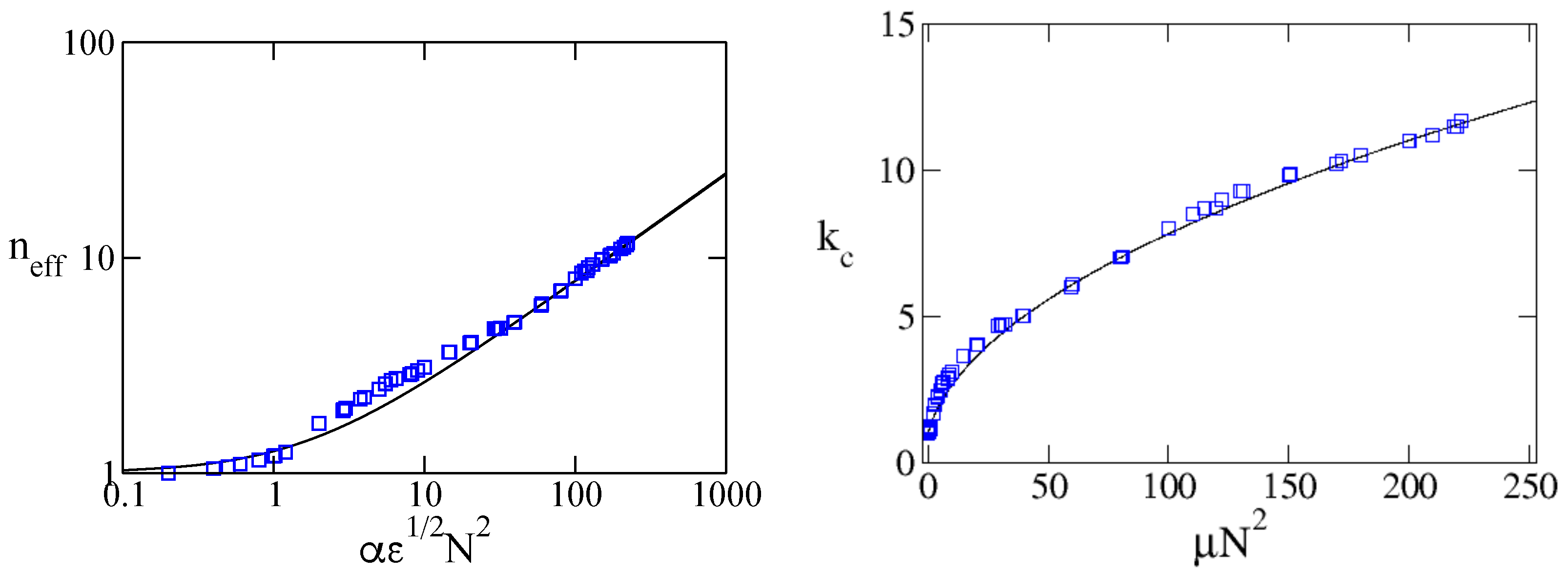
One is now in a position to quantitatively compare the central result obtained, Equation (27), with numerical results from Lin et al. [14]. The authors of that study measured the effective number,

$$n_{\mathrm{eff}}={\mathrm{e}}^S,S=-\sum _k{e}_{k}ln{e}_k,$$

(28)

which ranges from 1 to N as $S=0$ for one mode excited, and $S=lnN$ for equally distributed mode energies. According to the derivation made:

$$k_c=n_{\mathrm{eff}}.$$

(29)

In order to test the above equality, the data on $n_{\mathrm{eff}}$ versus $\mu N^2$ for $N=3,264,128$ are extracted from Figure 4 of Ref. [14]. The result is plotted in Figure 2 along with the theoretical result for $k_c$ in Equation (27). Very good agreement can be observed.

One concludes that the FPUT trajectory will, for long times, excite a mode packet with $k_c$ modes, which are the core modes of the packet. The remaining $(N-k_c)$ modes belong to the tail of the packet, and decay exponentially with increasing k. Let us further note that the theoretical result obtained here can be rewritten in the limit of large system size as:

$$\frac{k_c}{N}\approx \frac{\sqrt{6\alpha }}{\pi }{\epsilon }^{1/4},\epsilon =\frac{E}{N},N\gg 1.$$

(30)

Therefore, the packet size becomes system size-independent if expressed entirely through intensive quantities—wave numbers and energy densities.

5. Discussion

It is now understood that both FPUT recurrences and super-recurrences are part of the dynamics of so-called metastable states (mode packets) [22], which eventually relax into equipartition at some time $T_2$. These metastable states are formed at a time $T_1$, persisting over potentially huge time intervals, ∼$(T_2-T_1)$. They are characterized by a localized distribution of energy in mode space. This distribution has a core which, e.g., in the case of the original FPUT test, contains a few low-frequency modes. The distribution has also a tail. Galgani and Scott observed that this tail is exponentially decaying [21]. The distribution appears to be almost stationary when using proper averaging times which are much shorter than $T_m$, though of course lots of dynamics is going on at various time scales, e.g., recurrences and super-recurrences. The core shows recurrence and super-recurrence, but also various forms of chaos (at even larger time scales). The tails are characterized by decay structures in normal mode space, resonances, and slow incoherent heating. The decay structures can be exponential, thus leading to length scales in normal mode space or algebraic implying the absence of the latter. Resonances in the decay profiles show the driven nature of these tails, with the core being the driving source. Incoherent heating results from the same core driving, which at larger time scales may exhibit chaotic incoherent dynamics.

The core dynamics are quantified by their recurrence, $T_{\mathrm{R}}$, and super-recurrence, $T_{\mathrm{SR}}$, times and the core size. While the recurrence and super-recurrence times were assessed in previous studies a quantitative calculation of the core size is provided here, which agrees very well with the measured data. One can therefore conclude that the regular core dynamics have been to some extent exhaustively studied. What remains for the core is to assess its chaotic incoherent dynamics. These dynamics are the reason for the slow heating of the tail modes, and will ultimately explain the time scale $T_2$ of a final reaching of equipartition, as studied numerically in detail in Ref. [23].

6. Conclusions

In this paper, a quantitative estimates for the size of the core and tail of a low-frequency, normal-mode excitation in a Fermi–Pasta–Ulam–Tsingou (FPUT) chain is provided. How will these results be modified if high frequency modes are excited? Even more intriguing is the question of whether any of these results are carried over in some form for an FPUT system at thermal equilibrium—what are the details of the energy transfer between low and high frequency modes in such a situation? What will happen at higher lattice dimensions? What changes if the model supports optical normal modes with a finite frequency gap in the band structure? It seems there a plenty of questions to be addressed 70 years after the FPUT experiment.

7. HB2U

I had a great time working together with Mikhail Tribelsky back in Dresden at the Max Planck Institute for Physics of Complex Systems. We both shared a passion for puzzles and paradoxes, probably intuitively realizing that however remote the topic of the puzzle is, solving it will advance the mind in potentially unexpected areas of science and general understanding of the world. I dedicate this paper to Mikhail’s 70th birthday. It solves some aspects of a paradox which is almost the same age, paradoxically.

References

- Fermi, E.; Pasta, J.; Ulam, S. Studies of the nonlinear problems. I. LASL Report LA-1940; Los Alamos Scientific Laboratory: Los Alamos, CA, USA, 1955; Reprinted in The Collected Papers of Enrico Fermi; Segré, E., Ed.; University of Chicago Press: Chicago, IL, USA, 1965; Volume II. [Google Scholar] [CrossRef] [Green Version]
- Ford, J. The Fermi–Pasta-Ulam problem: Paradox turns discovery. Phys. Rep. 1992, 213, 271–310. [Google Scholar] [CrossRef]
- Weissert, T.P. The Genesis of Simulation in Dynamics: Pursuing the Fermi–Pasta-Ulam Problem; Springer: New York, NY, USA, 1997. [Google Scholar]
- Campbell, D.K.; Rosenau, P.; Zaslavsky, G. Introduction: The Fermi-Pasta-Ulam problem—The first fifty years. Chaos 2005, 15, 015101. [Google Scholar] [CrossRef] [PubMed]
- Gallavotti, G. The Fermi–Pasta-Ulam Problem: A Status Report; Springer: Berlin/Heidelberg, Germany, 2007. [Google Scholar]
- Zabusky, N.J. Exact solution for the vibrations of a nonlinear continuous model string. J. Math. Phys. 1962, 3, 1028–1039. [Google Scholar] [CrossRef]
- Kruskal, M.D.; Zabusky, N.J. Stroboscopic-perturbation procedure for treating a class of nonlinear wave equations. J. Math. Phys. 1964, 5, 231–244. [Google Scholar] [CrossRef]
- Zabusky, N.J.; Kruskal, M.D. Interaction of “solitons” in a collisionless plasma and the recurrence of initial states. Phys. Rev. Lett. 1965, 15, 240–243. [Google Scholar] [CrossRef] [Green Version]
- Ford, J. Equipartition of energy for nonlinear systems. J. Math. Phys. 1961, 2, 387–393. [Google Scholar] [CrossRef]
- Jackson, E.A. Nonlinear coupled oscillators. I. Perturbation theory; Ergodic Problem. J. Math. Phys. 1963, 4, 551–558. [Google Scholar] [CrossRef]
- Jackson, E.A. Nonlinear coupled oscillators. II. Comparison of theory with computer solutions. J. Math. Phys. 1963, 4, 686–700. [Google Scholar] [CrossRef]
- Tuck, J.; Menzel, M. The superperiod of the nonlinear weighted string (FPU) problem. Adv. Math. 1972, 9, 399–407. [Google Scholar] [CrossRef] [Green Version]
- Sholl, D.S.; Henry, B. Recurrence times in cubic and quartic Fermi–Pasta-Ulam chains: A shifted-frequency perturbation treatment. Phys. Rev. A 1991, 44, 6364. [Google Scholar] [CrossRef] [PubMed]
- Lin, C.; Goedde, C.; Lichter, S. Scaling of the recurrence time in the cubic Fermi–Pasta-Ulam lattice. Phys. Lett. A 1997, 229, 367–374. [Google Scholar] [CrossRef]
- Flach, S.; Ivanchenko, M.; Kanakov, O. q-Breathers and the Fermi–Pasta-Ulam problem. Phys. Rev. Lett. 2005, 95, 064102. [Google Scholar] [CrossRef] [PubMed] [Green Version]
- Flach, S.; Ivanchenko, M.; Kanakov, O. q-Breathers in Fermi–Pasta-Ulam chains: Existence, localization, and stability. Phys. Rev. E 2006, 73, 036618. [Google Scholar] [CrossRef] [PubMed] [Green Version]
- Ponno, A.; Christodoulidi, H.; Skokos, C.; Flach, S. The two-stage dynamics in the Fermi–Pasta-Ulam problem: From regular to diffusive behavior. Chaos Interdiscip. J. Nonlinear Sci. 2011, 21, 043127. [Google Scholar] [CrossRef] [PubMed] [Green Version]
- Pace, S.D.; Campbell, D.K. Behavior and breakdown of higher-order Fermi–Pasta-Ulam-Tsingou recurrences. Chaos Interdiscip. J. Nonlinear Sci. 2019, 29, 023132. [Google Scholar] [CrossRef] [PubMed] [Green Version]
- De Luca, J.; Lichtenberg, A.J.; Lieberman, M.A. Time scale to ergodicity in the Fermi–Pasta-Ulam system. Chaos 1995, 5, 283–297. [Google Scholar] [CrossRef] [PubMed]
- Zygmund, A. Trigonometric Series; Cambridge University Press: Cambridge, UK, 1968. [Google Scholar]
- Galgani, L.; Scott, A. Planck-like distributions in classical nonlinear mechanics. Phys. Rev. Lett. 1972, 28, 1173. [Google Scholar] [CrossRef]
- Benettin, G.; Carati, A.; Galgani, L.; Giorgilli, A. The Fermi-Pasta-Ulam problem and the metastability perspective. In The Fermi–Pasta-Ulam Problem; Gallavotti, G., Ed.; Springer: Berlin/Heidelberg, Germany, 2007; pp. 151–189. [Google Scholar] [CrossRef]
- Danieli, C.; Campbell, D.; Flach, S. Intermittent many-body dynamics at equilibrium. Phys. Rev. E 2017, 95, 060202. [Google Scholar] [CrossRef] [PubMed] [Green Version]
Figure 1.
Evolution of the linear mode energies for the first five modes on a large timescale for the original Fermi–Pasta–Ulam-Tsingou (FPUT) trajectory for the parameter , and the number of particles [1] (oscillating curves). The almost-straight horizontal lines indicate the weak time dependence of the linear mode energies on corresponding exact time-periodic q-breather solutions from [16]. Figure is adapted from [16].
Figure 2.
(Left panel) The effective number, versus with . The symbols represent the data read off from Figure 4b of Ref. [14], correspond to a set of different system sizes, , and demonstrate a single scaling curve existence. The black line represents the theoretical result (27). (Right panel) same as left panel but using linear scales. The square-root law of Equation (27) provides an extremely good fit.
Publisher’s Note: MDPI stays neutral with regard to jurisdictional claims in published maps and institutional affiliations. |
© 2021 by the author. Licensee MDPI, Basel, Switzerland. This article is an open access article distributed under the terms and conditions of the Creative Commons Attribution (CC BY) license (https://creativecommons.org/licenses/by/4.0/).
Share and Cite
MDPI and ACS Style
Flach, S. Measuring α-FPUT Cores and Tails. Physics 2021, 3, 879-887. https://doi.org/10.3390/physics3040054
AMA Style
Flach S. Measuring α-FPUT Cores and Tails. Physics. 2021; 3(4):879-887. https://doi.org/10.3390/physics3040054
Chicago/Turabian StyleFlach, Sergej. 2021. "Measuring α-FPUT Cores and Tails" Physics 3, no. 4: 879-887. https://doi.org/10.3390/physics3040054
APA StyleFlach, S. (2021). Measuring α-FPUT Cores and Tails. Physics, 3(4), 879-887. https://doi.org/10.3390/physics3040054