Refinement Orders for Quantitative Information Flow and Differential Privacy ^†

Abstract

Quantitative Information Flow (QIF) and Differential Privacy (DP) are both concerned with the protection of sensitive information, but they are rather different approaches. In particular, QIF considers the expected probability of a successful attack, while DP (in both its standard and local versions) is a max-case measure, in the sense that it is compromised by the existence of a possible attack, regardless of its probability. Comparing systems is a fundamental task in these areas: one wishes to guarantee that replacing a system A by a system B is a safe operation that is the privacy of B is no worse than that of A. In QIF, a refinement order provides strong such guarantees, while, in DP, mechanisms are typically compared w.r.t. the privacy parameter $\epsilon$ in their definition. In this paper, we explore a variety of refinement orders, inspired by the one of QIF, providing precise guarantees for max-case leakage. We study simple structural ways of characterising them, the relation between them, efficient methods for verifying them and their lattice properties. Moreover, we apply these orders in the task of comparing DP mechanisms, raising the question of whether the order based on $\epsilon$ provides strong privacy guarantees. We show that, while it is often the case for mechanisms of the same “family” (geometric, randomised response, etc.), it rarely holds across different families.

1. Introduction

The enormous growth in the use of internet-connected devices and the big-data revolution have created serious privacy concerns, and motivated an intensive area of research aimed at devising methods to protect the users’ sensitive information. During the last decade, two main frameworks have emerged in this area: Differential Privacy (DP) and Quantitative Information Flow (QIF).

Differential privacy (DP) [1] was originally developed in the area of statistical databases, and it aims at protecting the individuals’ data while allowing the release of aggregate information through queries. This is obtained by obfuscating the result of the query via the addition of controlled noise. Naturally, we need to assume that the curator, namely the entity collecting and storing the data and handling the queries, is honest and capable of protecting the data from security breaches. Since this assumption cannot always be guaranteed, a variant has been proposed: local differential privacy (LDP) [2], where the data are obfuscated individually before they are collected.

Both DP and LPD are subsumed by $\mathit{d}$-privacy [3], and, in this paper, we will use the latter as a unifying framework. The definition of $\mathit{d}$-privacy assumes an underlying metric structure on the data domain $\mathcal{X}$. An obfuscation mechanism K for $\mathcal{X}$ is a probabilistic mapping from $\mathcal{X}$ to some output domain $\mathcal{Y}$, namely a function from $\mathcal{X}$ to probabilistic distributions over $\mathcal{Y}$. We will use the notation $K_{x,y}$ to represent the probability that K on input x gives output y. The mechanism K is $\epsilon ·\mathit{d}$-private, where $\epsilon$ is a parameter representing the privacy level, if

$$K_{x_1,y}\le e^{\epsilon \mathit{d}(x_1,x_2)}{K}_{x_2,y}\mathrm{for}\mathrm{all}{x}_1,x_2\in \mathcal{X},y\in \mathcal{Y}$$

(1)

Standard DP is obtained from this definition by assuming $\mathcal{X}$ to be a set of all datasets and $\mathit{d}$ the Hamming distance between two datasets, seen as vectors or records (i.e., the number of positions in which the two datasets differ). Note that the more common definition of differential privacy assumes that $x_1,x_2$ are adjacent, i.e., their Hamming distance is 1, and requires $K_{x_1,y}\le e^{\epsilon }{K}_{x_2,y}$. It is easy to prove that the two definitions are equivalent. As for LDP, it is obtained by considering the so-called discrete metric which assigns distance 0 to identical elements, and 1 otherwise.

The other framework for the protection of sensitive information, quantitative information flow (QIF), focuses on the potentialities and the goals of the attacker, and the research on this area has developed rigorous foundations based on information theory [4,5]. The idea is that a system processing some sensitive data from a random variable X and releasing some observable data as a random variable Y can be modelled as an information-theoretic channel with input X and output Y. The leakage is then measured in terms of correlation between X and Y. There are, however, many different ways to define such correlation, depending on the notion of adversary. In order to provide a unifying approach, Ref. [6] has proposed the theory of g-leakage, in which an adversary is characterized by a functional parameter g representing its gain for each possible outcomes of the attack.

One issue that arises in both frameworks is how to compare systems from the point of view of their privacy guarantees. It is important to have a rigorous and effective way to establish whether a mechanism is better or worse than another one, in order to guide the design and the implementation of mechanisms for information protection. This is not always an obvious task. To illustrate the point, consider the following examples.

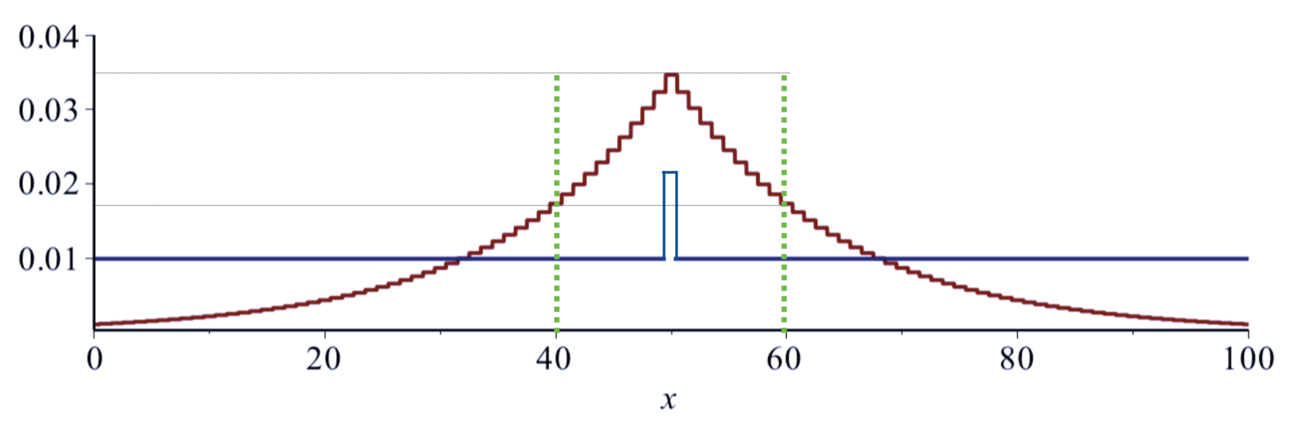
Example 1.

Let $P_1,P_2,P_3$ and $P_4$ be the programs illustrated in Table 1, whereHis a “high” (i.e., secret) input andLis a “low” (i.e., public) output. We assume thatHis a uniformly distributed 32-bit integer with range $0\le \mathtt{H}<2^{32}$. All these programs leak information aboutHviaL, in different ways: $P_1$ revealsHwhenever it is a multiple of 8 (H mod 8represents the integer division ofHby 8), and reveals nothing otherwise. $P_2$ does the same thing wheneverHis a multiple of 4. $P_3$ reveals the last 8 bits ofH(note thatH$\&{\mathtt{0}}^{\mathtt{24}}{\mathtt{1}}^{\mathtt{8}}$ represents the bitwise conjunction betweenHand a string of 24 bits “0” followed by 8 bits “1”). Analogously, $P_4$ reveals the last 4 bits ofH. Now, it is clear that $P_2$ leaks more than $P_1$, and that $P_4$ leaks more than $P_3$, but how to compare, for instance, $P_1$, and $P_3$? It is debatable which one is worse because their behavior is very different: $P_1$ reveals nothing in most cases, but when it does reveal something, it reveals everything. $P_3$, on the other hand, always reveals part of the secret. Clearly, we cannot decide which situation is worse, unless we have some more information about the goals and the capabilities of the attacker. For instance, if the adversary has only one attempt at his disposal (and no extra information), then the program $P_3$ is better because even after the output ofLthere are still 24 bits ofHthat are unknown. On the other hand, if the adversary can repeat the attacks on program similar to $P_3$, then eventually it will uncover the secret entirely all the times.

Table 1. Programs that take in input a secret H and leak information about H via the output L.

${\mathit{P}}_1$	${\mathit{P}}_2$	${\mathit{P}}_3$	${\mathit{P}}_4$
if H mod 8 = 0 then	if H mod 4 = 0 then	L := H $\&{\mathtt{0}}^{\mathtt{24}}{\mathtt{1}}^{\mathtt{8}}$	L := H $\&{\mathtt{0}}^{\mathtt{28}}{\mathtt{1}}^{\mathtt{4}}$
L := H	L := H
else	else
L := 1	L := 1

Example 2.

Consider the domain of the integer numbers between 0 and 100, and consider a geometric mechanism (cf. Definition 9) on this domain, with $\epsilon =\log \raisebox{1ex}{$27$}\!\left/ \!\raisebox{-1ex}{$25$}\right.$. Then, consider a randomized response mechanism (cf. Definition 13) still on the same domain and $\epsilon =\log 2$. The two mechanisms are illustrated in Figure 1. They both satisfy $\mathit{d}$-privacy, but for different $\mathit{d}$: in the first case $\mathit{d}$ is the standard distance between numbers, while in the second case it is the discrete metric. Clearly, it does not make sense to compare these mechanisms on the basis of their respective privacy parameters ε because they represent different privacy properties, and it is not obvious how to compare them in general: The geometric mechanism tends to make the true value indistinguishable from his immediate neighbors, but it separates it from the values far away. The randomized response introduces the same level of confusion between the true value and any other value of the domain. Thus, which mechanism is more private depends on the kind of attack we want to mitigate: if the attacker is trying to guess an approximation of the value, then the randomized response is better. If the attacker is only interested in identifying the true value among the immediate neighbors, then the geometric is better. Indeed, note that in the subdomain of the numbers between 40 and 60 the geometric mechanism also satisfies $\mathit{d}$-privacy with $\mathit{d}$ being the discrete metric and $\epsilon =\log 2$, and in any subdomain smaller than that it satisfies the discrete metric $\mathit{d}$-privacy with $\epsilon <\log 2$.

Figure 1. Comparison between the geometric (red) and the randomized response (blue) mechanisms. The area between 40 and 60, delimited by the green lines, represents the sub-domain where the geometric mechanism satisfies also the discrete metric $\mathit{d}$-privacy with $\epsilon =\log 2$.

In this respect, the QIF approach has led to an elegant theory of refinement (pre)order (In this paper, we call ${⊑}_{\mathbb{G}}^{\mathrm{avg}}$ and the other refinement relations “orders”, although, strictly speaking, they are preorders.) ${⊑}_{\mathbb{G}}^{\mathrm{avg}}$, which provides strong guarantees: $A{⊑}_{\mathbb{G}}^{\mathrm{avg}}B$ means that B is safer than A in all circumstances, in the sense that the expected gain of an attack on B is less than on A, for whatever kind of gain the attacker may be seeking. This means that we can always substitute the component A by B without compromising the security of the system. An appealing aspect of this particular refinement order is that it is characterized by a precise structural relation between the stochastic channels associated with A and B [6,7], which makes it easy to reason about, and relatively efficient to verify. It is important to remark that this order is based on an average notion of adversarial gain (vulnerability), defined by mediating over all possible observations and their probabilities. We call this perspective average-case.

At the other end of the spectrum, DP, LDP and $\mathit{d}$-privacy are max-case measures. In fact, by applying the Bayes theorem to (1), we obtain:

$$\frac{p(x_1\mid y)}{p(x_2\mid y)}\le e^{\epsilon \mathit{d}(x_1,x_2)}\frac{\pi \left(x_1\right)}{\pi \left(x_2\right)}\mathrm{for}\mathrm{all}{x}_1,x_2\in \mathcal{X},y\in \mathcal{Y}$$

(2)

where, for $i\in \{1,2\}$, $\pi \left(x_i\right)$ is the $prior$ probability of $x_i$ and $p(x_i\mid y)$ is the posterior probability of $x_i$ given y. We can interpret $\raisebox{1ex}{$\pi \left(x_1\right)$}\!\left/ \!\raisebox{-1ex}{$\pi \left(x_2\right)$}\right.$ and $\raisebox{1ex}{$p(x_1\mid y)$}\!\left/ \!\raisebox{-1ex}{$p(x_2\mid y)$}\right.$ as knowledge about $\mathcal{X}$: they represent how much more likely $x_1$ is with respect to $x_2$, before (prior) and after (posterior) observing y, respectively. Thus, the property expresses a bound on how much the adversary can learn from each individual outcome of the mechanism (The property (2) is also the semantic interpretation of the guarantees of the Pufferfish framework (cf. [8], Section 3.1). The ratio $\raisebox{1ex}{$\frac{p(x_1\mid y)}{p(x_2\mid y)}$}\!\left/ \!\raisebox{-1ex}{$\frac{\pi \left(x_1\right)}{\pi \left(x_2\right)}$}\right.$ is known as odds ratio).

In the literature of DP, LDP and $\mathit{d}$-privacy, mechanisms are usually compared on the basis of their $\epsilon$-value (In DP and LDP $\epsilon$ is a parameter that usually appears explicitly in the definition of the mechanism. In d-privacy, it is an implicit scaling factor.), which controls a bound on the log-likelihood ratio of an observation y given two “secrets” $x_1$ and $x_2$: smaller $\epsilon$ means more privacy. In DP and LDP, the bound is $\epsilon$ itself, while in $\mathit{d}$-privacy it is $\epsilon \times \mathit{d}(s_1,s_2)$ We remark that the relation induced by $\epsilon$ in $\mathit{d}$-privacy is fragile, in the sense that the definition of $\mathit{d}$-privacy assumes an underlying metric structure $\mathit{d}$ on the data, and whether a mechanism B is “better” than A depends in general on the metric considered.

Average-case and max-case are different principles, suitable for different scenarios: the former represents the point of view of an organization, for instance an insurance company providing coverage for risks related to credit cards, which for the cost–benefit analysis is interested in reasoning in terms of expectation (expected cost of an attack). The max-case represents the point of view of an individual, who is interested in limiting the cost of any attack. As such, the max-case seems particularly suitable for the domain of privacy.

In this paper, we combine the max-case perspective with the robustness of the QIF approach, and we introduce two refinement orders:

• ${⊑}_{\mathbb{Q}}^{\max }$, based on the max-case leakage introduced in [9]. This order takes into account all possible privacy breaches caused by any observable (like in the DP world), but it quantifies over all possible quasi-convex vulnerability functions (in the style of the QIF world).
• ${⊑}_{\mathbb{M}}^{\mathrm{prv}}$, based on $\mathit{d}$-privacy (like in the DP world), but quantified over all metrics $\mathit{d}$.

To underline the importance of a robust order, let us consider the case of the oblivious mechanisms for differential privacy: These mechanisms are of the form $K=H\circ f$, where $f:\mathcal{X}\to \mathcal{Y}$ is a query, namely a function from datasets in $\mathcal{X}$ to some answer domain $\mathcal{Y}$, and H is a probabilistic mechanism implementing the noise. The idea is that the system first computes the result $y\in \mathcal{Y}$ of the query (true answer), and then it applies H to y to obtain a reported answer z. In general, if we want K to be $\epsilon$-DP, we need to tune the mechanism H in order to take into account the sensitivity of f, which is the maximum distance between the results of f on two adjacent databases, and as such it depends on the metric on $\mathcal{Y}$. However, if we know that $K=H\circ f$ is $\epsilon$-DP, and that $H{⊑}_{\mathbb{M}}^{\mathrm{prv}}{H}^{\prime }$ for some other mechanism $H^{\prime }$, then we can safely substitute H by $H^{\prime }$ as it is because one of our results (cf. Theorem A5) guarantees that $K^{\prime }=H^{\prime }\circ f$ is also $\epsilon$-DP. In other words, $H{⊑}_{\mathbb{M}}^{\mathrm{prv}}{H}^{\prime }$ implies that we can substitute H by $H^{\prime }$ in an oblivious mechanism for whatever query f and whatever metric on $\mathcal{Y}$, without the need to know the sensitivity of f and without the need to do any tuning of $H^{\prime }$. Thanks to Theorems 3 and 4, we know that this is the case also for ${⊑}_{\mathbb{G}}^{\mathrm{avg}}$ and ${⊑}_{\mathbb{Q}}^{\max }$. We illustrate this with the following example.

Example 3.

Consider datasets $x\in \mathcal{X}$ of records containing the age of people, expressed as natural numbers from 0 to 100, and assume that each dataset in $\mathcal{X}$ contains at least 100 records. Consider two queries, $f\left(x\right)$ and $g\left(x\right)$, which give the rounded average age and the minimum age of the people in x, respectively. Finally, consider the truncated geometric mechanism $T{G}^{\epsilon }$ (cf. Definition 10), and the randomized response mechanism $R^{\epsilon }$ (cf. Definition 13). It is easy to see that $K_1=T{G}^{\epsilon }\circ f$ is ε-DP, and it is possible to prove that $T{G}^{\epsilon }{⊑}_{\mathbb{M}}^{\mathrm{prv}}{R}^{\epsilon }$ (cf. Theorem 14). We can then conclude that $K_2=R^{\epsilon }\circ f$ is ε-DP as well, and that in general it is safe to replace $T{G}^{\epsilon }$ by $R^{\epsilon }$ for whatever query. On the other hand, $R^{\epsilon }/{⊑}_{\mathbb{M}}^{\mathrm{prv}}T{G}^{\epsilon }$, so we cannot expect that it is safe to replace $R^{\epsilon }$ by $T{G}^{\epsilon }$ in any context. In fact, $K_3=R^{\epsilon }\circ g$ is ε-DP, but $K_4=T{G}^{\epsilon }\circ g$ isnotε-DP, despite the fact that both mechanisms are constructed using the same privacy parameter ε. Hence, we can conclude that a refinement relation based only on the comparison of the ε parameters would not be robust, at least not for a direct replacement in an arbitrary context. Note that $K_4$ is $100\times \epsilon$-DP. In order to make it ε-DP, we should divide the parameter ε by the sensitivity of g (with respect to the ordinary distance on natural numbers), which is 100, i.e., use $T{G}^{\raisebox{1ex}{$\epsilon $}\!\left/ \!\raisebox{-1ex}{$100$}\right.}$. For $R^{\epsilon }$, this is not necessary because it is defined using the discrete metric on $\{0,\dots ,100\}$, and the sensitivity of g with respect to this metric is 1.

The robust orders allow us to take into account different kinds of adversaries. The following example shows what the idea is.

Example 4.

Consider the following three LDP mechanisms, represented by their stochastic matrices (where each element is the conditional probability of the outcome of the mechanism, given the secret value). The secrets are three possible economic situations of an individual, p, a and r, standing for “poor”, “average” and “rich”, respectively. The observable outcomes are r and $\mathit{n}$, standing for “rich” and “not rich”.

$$\begin{array}{|ccc|}\hline A& n& r\\ p& \raisebox{1ex}{$3$}\!\left/ \!\raisebox{-1ex}{$4$}\right.& \raisebox{1ex}{$1$}\!\left/ \!\raisebox{-1ex}{$4$}\right.\\ a& \raisebox{1ex}{$1$}\!\left/ \!\raisebox{-1ex}{$2$}\right.& \raisebox{1ex}{$1$}\!\left/ \!\raisebox{-1ex}{$2$}\right.\\ r& \raisebox{1ex}{$1$}\!\left/ \!\raisebox{-1ex}{$4$}\right.& \raisebox{1ex}{$3$}\!\left/ \!\raisebox{-1ex}{$4$}\right.\\ \hline\end{array}\begin{array}{|ccc|}\hline B& n& r\\ p& \raisebox{1ex}{$2$}\!\left/ \!\raisebox{-1ex}{$3$}\right.& \raisebox{1ex}{$1$}\!\left/ \!\raisebox{-1ex}{$3$}\right.\\ a& \raisebox{1ex}{$2$}\!\left/ \!\raisebox{-1ex}{$3$}\right.& \raisebox{1ex}{$1$}\!\left/ \!\raisebox{-1ex}{$3$}\right.\\ r& \raisebox{1ex}{$1$}\!\left/ \!\raisebox{-1ex}{$3$}\right.& \raisebox{1ex}{$2$}\!\left/ \!\raisebox{-1ex}{$3$}\right.\\ \hline\end{array}\begin{array}{|ccc|}\hline C& n& r\\ p& \raisebox{1ex}{$2$}\!\left/ \!\raisebox{-1ex}{$3$}\right.& \raisebox{1ex}{$1$}\!\left/ \!\raisebox{-1ex}{$3$}\right.\\ a& \raisebox{1ex}{$1$}\!\left/ \!\raisebox{-1ex}{$2$}\right.& \raisebox{1ex}{$1$}\!\left/ \!\raisebox{-1ex}{$2$}\right.\\ r& \raisebox{1ex}{$1$}\!\left/ \!\raisebox{-1ex}{$3$}\right.& \raisebox{1ex}{$2$}\!\left/ \!\raisebox{-1ex}{$3$}\right.\\ \hline\end{array}$$

(3)

Let us assume that the prior distribution π on the secrets is uniform. We note that A is $\left(\log 3\right)$-LDP while B is $\left(\log 2\right)$-LDP. Hence, if we only look at the value of ε, we would think that B is better than A from the privacy point of view. However, there are attackers that gain more from B than from A (which means that, with respect to those attackers, the privacy of B is worse). For instance, this is the case when the attacker is only interested in discovering whether the person is rich or not. In fact, if we consider a gain 1 when the attacker guesses the right class (r versus (either p or a)) and 0 otherwise, we have that the highest possible gain in A is $\left(\raisebox{1ex}{$3$}\!\left/ \!\raisebox{-1ex}{$4$}\right.\right)\pi \left(p\right)+\left(\raisebox{1ex}{$1$}\!\left/ \!\raisebox{-1ex}{$2$}\right.\right)\pi \left(a\right)=\raisebox{1ex}{$5$}\!\left/ \!\raisebox{-1ex}{$12$}\right.$, while in B is $\left(\raisebox{1ex}{$2$}\!\left/ \!\raisebox{-1ex}{$3$}\right.\right)\pi \left(p\right)+\left(\raisebox{1ex}{$2$}\!\left/ \!\raisebox{-1ex}{$3$}\right.\right)\pi \left(a\right)=\raisebox{1ex}{$4$}\!\left/ \!\raisebox{-1ex}{$9$}\right.$, which is higher than $\raisebox{1ex}{$5$}\!\left/ \!\raisebox{-1ex}{$12$}\right.$. This is consistent with our orders: it is possible to show that none of the three orders hold between A and B, and that therefore we should not expect B to be better (for privacy) than A with respect to all possible adversaries.

On the other hand, the mechanism C is also $\left(\log 2\right)$-LDP, and in this case we have that the relation $A{⊑}_{\mathbb{Q}}^{\max }C$ holds, implying that we can safely replace A by C. We can also prove that the reverse does not hold, which means that C is strictly better than A.

A fundamental issue is how to prove that these robust orders hold: Since ${⊑}_{\mathbb{Q}}^{\max }$ and ${⊑}_{\mathbb{M}}^{\mathrm{prv}}$ involve universal quantifications, it is important to devise finitary methods to verify them. To this purpose, we will study their characterizations as structural relations between stochastic matrices (representing the mechanisms to be compared), along the lines of what was done for ${⊑}_{\mathbb{G}}^{\mathrm{avg}}$.

We will also study the relation between the three orders (the two above and ${⊑}_{\mathbb{G}}^{\mathrm{avg}}$), and their algebraic properties. Finally, we will analyze various mechanisms for DP, LDP, and $\mathit{d}$-privacy to see in which cases the order induced by $\epsilon$ is consistent with the three orders above.

1.1. Contribution

The main contributions of this paper are the following:

• We introduce two refinement orders for the max case, ${⊑}_{\mathbb{Q}}^{\max }$ and ${⊑}_{\mathbb{M}}^{\mathrm{prv}}$, that are robust with respect to a large class of adversaries.
• We give structural characterizations of both ${⊑}_{\mathbb{Q}}^{\max }$ and ${⊑}_{\mathbb{M}}^{\mathrm{prv}}$ in terms of relations on the stochastic matrices of the mechanisms under comparison. These relations help the intuition and open the way to verification.
• We study efficient methods to verify the structural relations above. Furthermore, these methods are such that, when the verification fails, they produce counterexamples. In this way, it is possible to pin down what the problem is and try to correct it.
• We show that ${⊑}^{\mathrm{avg}}\subset {⊑}^{\max }\subset {⊑}^{\mathrm{prv}}$.
• We apply the three orders (${⊑}_{\mathbb{G}}^{\mathrm{avg}}$, ${⊑}_{\mathbb{Q}}^{\max }$, and ${⊑}_{\mathbb{M}}^{\mathrm{prv}}$) to the comparison of some well-known families of $\mathit{d}$-private mechanisms: geometric, exponential and randomised response. We show that, in general, $A{⊑}_{\mathbb{G}}^{\mathrm{avg}}B$ (and thus all the refinement orders between A and B) holds within the same family whenever the $\epsilon$ of B is smaller than that of A.
• We show that, if A and B are mechanisms from different families, then, even if the $\epsilon$ of B is smaller than that of A, the relations $A{⊑}_{\mathbb{G}}^{\mathrm{avg}}B$ and $A{⊑}_{\mathbb{Q}}^{\max }B$ do not hold, and in most cases $A{⊑}_{\mathbb{M}}^{\mathrm{prv}}B$ does not hold either. We conclude that a comparison based only on the value of the $\epsilon$’s is not robust across different families, at least not for the purposes illustrated above.
• We study lattice-properties of these orders. In contrast to ${⊑}_{\mathbb{G}}^{\mathrm{avg}}$, which was shown to not be a lattice, we prove that suprema and infima exist for ${⊑}_{\mathbb{Q}}^{\max }$ and ${⊑}_{\mathbb{M}}^{\mathrm{prv}}$, and that therefore these orders form lattices.

1.2. Related Work

We are not aware of many studies on refinement relations for QIF. Yasuoka and Terauchi [10] and Malacaria [11] have explored strong orders on deterministic mechanisms, focusing on the fact that such mechanisms induce partitions on the space of secrets. They showed that the orders produced by min-entropy leakage [5] and Shannon leakage [12,13] are the same and, moreover, they coincide with the partition refinement order in the Lattice of Information [14]. This order was extended to the probabilistic case in [6], resulting in the relation ${⊑}^{\mathrm{avg}}$ mentioned in Section 2. The same paper [6] proposed the theory of g-leakage and introduced the corresponding order ${⊑}_{\mathbb{G}}^{\mathrm{avg}}$. Furthermore, [6] proved that ${⊑}^{\mathrm{avg}}\subseteq {⊑}_{\mathbb{G}}^{\mathrm{avg}}$ and conjectured that also the reverse should hold. This conjecture was then proved valid in [7]. The max-case leakage, on which the relation ${⊑}_{\mathbb{Q}}^{\max }$ is based, was introduced in [9], but ${⊑}_{\mathbb{Q}}^{\max }$ and its properties were not investigated. Finally, ${⊑}^{\mathrm{prv}}$ is a novel notion introduced in this paper.

In the field of differential privacy, on the other hand, there have been various works aimed at trying understand the operational meaning of the privacy parameter $\epsilon$ and at providing guidelines for the choice of its values. We mention, for example [15,16], which consider the value of $\epsilon$ from an economical point of view, in terms of cost. We are not aware, however, of studies aimed at establishing orders between the level of privacy of different mechanisms, except the one based on the comparison of the $\epsilon$’s.

The relation between QIF and DP, LDP, and $\mathit{d}$-privacy is based on the so-called semantic interpretation of the privacy notions that regard these properties as expressing a bounds on the increase of knowledge (from prior to posterior) due to the answer reported by the mechanism. For $\mathit{d}$-privacy, the semantic interpretation is expressed by (2). To the best of our knowledge, this interpretation was first pointed out (for the location privacy instance) in [17]. The seminal paper on $\mathit{d}$-privacy, [3], also proposed a semantic interpretation, with a rather different flavor, although formally equivalent. As for DP, as explained in the Introduction, (2) instantiated to databases and Hamming distance corresponds to the odds ratio on which the semantics interpretation is based provided in [8]. Before that, another version of semantic interpretation was presented in [1] and proved equivalent to a form of DP called $\epsilon$-indistinguishability. Essentially, in this version, an adversary that queries the database, and knows all the database except one record, cannot infer too much about this record from the answer to the query reported by the mechanism. Later on, an analogous version of semantic interpretation was reformulated in [18] and proved equivalent to DP. A different interpretation of DP, called semantic privacy, was proposed by [19]. This interpretation is based on a comparison between two posteriors (rather between the posterior and the prior), and the authors show that, within certain limits, it is equivalent to DP.

A short version of this paper, containing only some of the proofs, appeared in [20].

1.3. Plan of the Paper

In the next three sections, Section 2, Section 3 and Section 4, we define the order refinements ${⊑}_{\mathbb{G}}^{\mathrm{avg}}$, ${⊑}_{\mathbb{Q}}^{\max }$ and ${⊑}_{\mathbb{M}}^{\mathrm{prv}}$, respectively, and we study their properties. In Section 5.1, we investigate methods to verify them. In Section 6, we consider various mechanisms for DP and its variants, and we investigate the relation between the parameter $\epsilon$ and the orders introduced in this paper. In Section 7, we show that ${⊑}_{\mathbb{Q}}^{\max }$ and ${⊑}_{\mathbb{M}}^{\mathrm{prv}}$ form a lattice. Finally, Section 8 provides conclusions.

Note: In order to make the reading of the paper more fluid, we have moved all the proofs to the appendix at the end of the paper.

2. Average-Case Refinement

We recall here some basic concepts from the literature. Table 2 lists the symbols used for the main concepts through the paper.

Table 2. Definitions and symbols used in this paper.

Defn	Vulnerabilities
Equation (4)	$V[\pi ,C]:={\sum }_y{a}_{y}V\left({\delta }^y\right)$
Section 3	$V^{\max }[\pi ,C]:={\max }_{y}V\left({\delta }^y\right)$
Definition 8	$V_{\mathit{d}}\left(\pi \right):=\inf \{\epsilon \ge 0|\forall x,x^{\prime }\in \mathcal{X},{\pi }_x\le e^{\epsilon ·\mathit{d}(x,x^{\prime })}{\pi }_{x^{\prime }}\}$
Defn	Leakage Measures
Definition 4	${\mathrm{Priv}}_{\mathit{d}}\left(C\right):=\inf \{\epsilon \ge 0|C\mathrm{satisfies}\epsilon ·\mathit{d}-\mathrm{privacy}\}$
Equation (23)	${\mathcal{L}}_{\mathit{d}}^{+,\max }(\pi ,C):=V_{\mathit{d}}^{\max }[\pi ,C]-V_{\mathit{d}}\left(\pi \right)$
Equation (24)	$\mathcal{M}{\mathcal{L}}_{\mathit{d}}^{+,\max }\left(C\right):={\max }_{\pi }{\mathcal{L}}_{\mathit{d}}^{+,\max }(\pi ,C)$
Defn	Refinement Orders
Equation (6)	$A{⊑}^{\mathrm{avg}}B\mathrm{iff}AR=B$ for some channel R
Definition 2	$A{⊑}^{\max }B\mathrm{iff}R\tilde{A}=\tilde{B}$ for some channel R
Definition 7	$A{⊑}^{\mathrm{prv}}B$ iff B satisfies ${\mathit{d}}_A$-privacy
Defn	Leakage Orders
Section 2.2	$A{⊑}_{\mathbb{G}}^{\mathrm{avg}}B\mathrm{iff}\forall g:\mathbb{G}\mathcal{X},\forall \pi :\mathbb{D}\mathcal{X},V_g[\pi ,A]\ge V_g[\pi ,B]$
Definition 1	$A{⊑}_{\mathbb{Q}}^{\max }B\mathrm{iff}\forall V:\mathbb{Q}\mathcal{X},\forall \pi :\mathbb{D}\mathcal{X},V^{\max }[\pi ,A]\ge V^{\max }[\pi ,B]$
Definition 6	$A{⊑}_{\mathbb{M}}^{\mathrm{prv}}B\mathrm{iff}\forall \mathit{d}\in \mathbb{M}\mathcal{X},A{⊑}_{\mathit{d}}^{\mathrm{prv}}B$
Definition 5	$A{⊑}_{\mathit{d}}^{\mathrm{prv}}B\mathrm{iff}{\mathrm{Priv}}_{\mathit{d}}\left(A\right)\ge {\mathrm{Priv}}_{\mathit{d}}\left(B\right)$

2.1. Vulnerability, Channels, and Leakage

Quantitative Information Flow studies the problem of quantifying the information leakage of a system (e.g., a program, or an anonymity protocol). A common model in this area is to consider that the user has a secret x from a finite set of possible secrets $\mathcal{X}$, about which the adversary has some probabilistic knowledge $\pi :\mathbb{D}\mathcal{X}$ ($\mathbb{D}\mathcal{X}$ denoting the set of probability distributions over $\mathcal{X}$). A function $V:\mathbb{D}\mathcal{X}\to {\mathbb{R}}_{\ge 0}$ is then employed to measure the vulnerability of our system: $V\left(\pi \right)$ quantifies the adversary’s success in achieving some desired goal, when his knowledge about the secret is $\pi$.

Various such functions can be defined (e.g., employing well-known notions of entropy), but it quickly becomes apparent that no single vulnerability function is meaningful for all systems. The family of g-vulnerabilities [6] tries to address this issue by parametrizing V in an operational scenario: first, the adversary is assumed to possess a set of actions $\mathcal{W}$; second, a gain function $g(w,x)$ models the adversary’s gain when choosing action w and the real secret is x. g-vulnerability can be then defined as the expected gain of an optimal guess: $V_g\left(\pi \right)={\max }_{w:\mathcal{W}}{\sum }_{x:\mathcal{X}}{\pi }_{x}g(w,x)$. Different adversaries can be modelled by proper choices of $\mathcal{W}$ and g. We denote by $\mathbb{G}\mathcal{X}$ the set of all gain functions.

A system is then modelled as a channel: a probabilistic mapping from the (finite) set of secrets $\mathcal{X}$ to a finite set of observations $\mathcal{Y}$, described by a stochastic matrix C, where $C_{x,y}$ is the probability that secret x produces the observation y. When the adversary observes y, he can transform his initial knowledge $\pi$ into a posterior knowledge ${\delta }^y:\mathbb{D}\mathcal{X}$. Since each observation y is produced with some probability $a_y$, it is sometimes conceptually useful to consider that the result of running a channel C, on the initial knowledge $\pi$, is a “hyper” distribution $[\pi ,C]$: a probability distribution on posteriors ${\delta }^y$, each having probability $a_y$.

It is then natural to define the (average-case) posterior vulnerability of the system by applying V to each posterior ${\delta }^y$, then averaging by its probability $a_y$ of being produced:

$$V[\pi ,C]:={\sum }_y{a}_{y}V\left({\delta }^y\right)$$

(4)

when defining vulnerability in this way, it can be shown [9] that V has to be convex on π; otherwise, fundamental properties (such as the data processing inequality) are violated. Any continuous and convex function V can be written as $V_g$ for a properly chosen g, so, when studying average-case leakage, we can safely restrict to using g-vulnerability.

Leakage can be finally defined by comparing the prior and posterior vulnerabilities, e.g., as ${\mathcal{L}}_g^{+}(\pi ,C)=V_g[\pi ,C]-V_g\left(\pi \right)$. (Comparing vulnerabilities “multiplicatively” is also possible but is orthogonal to the goals of this paper.)

2.2. Refinement

A fundamental question arises in the study of leakage: can we guarantee that a system B is no less safe than a system A? Having a family of vulnerability functions, we can naturally define a strong order ${⊑}_{\mathbb{G}}^{\mathrm{avg}}$ on channels by explicitly requiring that B leaks (Note that comparing the leakage of $A,B$ is equivalent to comparing their posterior vulnerability, so we choose the latter for simplicity.) no more than A, for all priors $\pi$ and all gain functions $g:\mathbb{G}\mathcal{X}$: (Note also that quantifying over $g:\mathbb{G}\mathcal{X}$ is equivalent to quantifying over all continuous and convex vulnerabilities.)

$$\begin{array}{cc}\hfill A{⊑}_{\mathbb{G}}^{\mathrm{avg}}B\mathrm{iff}& V_g[\pi ,A]\ge V_g[\pi ,B]\mathrm{for}\mathrm{all}g:\mathbb{G}\mathcal{X},\pi :\mathbb{D}\mathcal{X}\hfill \end{array}$$

(5)

Although ${⊑}_{\mathbb{G}}^{\mathrm{avg}}$ is intuitive and provides clear leakage guarantees, the explicit quantification over vulnerability functions makes it hard to reason about and verify. Thankfully, this order can be characterized in a “structural” way that is as a direct property of the channel matrix. We first define the refinement order ${⊑}^{\mathrm{avg}}$ on channels by requiring that B can be obtained by post-processing A by some other channel R that is:

$$A{⊑}^{\mathrm{avg}}B\mathrm{iff}AR=B\mathrm{for}\mathrm{some}\mathrm{channel}\mathrm{R}$$

(6)

A fundamental result [6,7] states that ${⊑}^{\mathrm{avg}}$ and ${⊑}_{\mathbb{G}}^{\mathrm{avg}}$ coincide.

We read $A{⊑}^{\mathrm{avg}}B$ as “A is refined by B”, or “B is as safe as A”. When $A{⊑}^{\mathrm{avg}}B$ holds, we have a strong privacy guarantee: we can safely replace A by B without decreasing the privacy of the system, independently from the adversary’s goals and his knowledge. However, refinement can be also useful in case $A/ {⊑}^{\mathrm{avg}}B$; namely, we can conclude that some adversary must exist, modelled by a gain function g, and some initial knowledge $\pi$, such that the adversary actually prefers to interact with A rather than interacting with B. (Whether this adversary is of practical interest or not is a different issue, but we know that one exists.) Moreover, we can actually construct such a “counter-example” gain function; this is discussed in Section 5.

3. Max-Case Refinement

Although ${⊑}^{\mathrm{avg}},{⊑}_{\mathbb{G}}^{\mathrm{avg}}$ provides a strong and precise way of comparing systems, one could argue that average-case vulnerability might underestimate the threat of a system. More precisely, imagine that there is a certain observation y such that the corresponding posterior ${\delta }^y$ is highly vulnerable (e.g., the adversary can completely infer the real secret), but y happens with very small probability $a_y$. In this case, the average-case posterior vulnerability $V[\pi ,C]$ can be relatively small, although $V\left({\delta }^y\right)$ is large for that particular y.

If such a scenario is considered problematic, we can naturally quantify leakage using a max-case (called “worse”-case in some contexts, although the latter is more ambiguous, “worse” can refer to a variety of factors.) variant of posterior vulnerability, where all observations are treated equally regardless of their probability of being produced:

$$V^{\max }[\pi ,C]:={\max }_{y}V\left({\delta }^y\right)$$

(7)

Under this definition, it can be shown [9] that V has to be quasi-convex on $\pi$ (instead of convex), in order to satisfy fundamental properties (such as the data processing inequality). Hence, in the max-case, we no longer restrict to g-vulnerabilities (which are always convex), but we can use any vulnerability $V:\mathbb{Q}\mathcal{X}$, where $\mathbb{Q}\mathcal{X}$ denotes the set of all continuous quasi-convex functions $\mathbb{D}\mathcal{X}\to {\mathbb{R}}_{\ge 0}$.

Inspired by ${⊑}_{\mathbb{G}}^{\mathrm{avg}}$, we can now define a corresponding max-case leakage order.

Definition 1.

The max-case leakage order is defined as

$$\begin{array}{ccc}\hfill A{⊑}_{\mathbb{Q}}^{\max }B\mathrm{iff}& V^{\max }[\pi ,A]\ge V^{\max }[\pi ,B]\hfill & \hfill \mathrm{for}\mathrm{all}V:\mathbb{Q}\mathcal{X},\pi :\mathbb{D}\mathcal{X}\end{array}$$

(8)

Similarly to its average-case variant, ${⊑}_{\mathbb{Q}}^{\max }$ provides clear privacy guarantees by explicitly requiring that B leaks no more than A for all adversaries (modelled as a vulnerability V). However, this explicit quantification makes the order hard to reason about and verify. We would thus like to characterize ${⊑}_{\mathbb{Q}}^{\max }$ by a refinement order that depends only on the structure of the two channels.

Given a channel C from $\mathcal{X}$ to $\mathcal{Y}$, we denote by $\tilde{C}$ the channel obtained by normalizing C’s columns (if a column consists of only zeroes, it is simply removed.) and then transposing:

$${\tilde{C}}_{y,x}:=\frac{C_{x,y}}{{\sum }_x{C}_{x,y}}$$

(9)

Note that the row y of $\tilde{C}$ can be seen as the posterior distribution ${\delta }^y$ obtained by C under the uniform prior. Note also that $\tilde{C}$ is non-negative and its rows sum up to 1, so it is a valid channel from $\mathcal{Y}$ to $\mathcal{X}$. The average-case refinement order required that B can be obtained by post-processing A. We define the max-case refinement order by requiring that $\tilde{B}$ can be obtained by pre-processing $\tilde{A}$.

Definition 2.

The max-case refinement order is defined as $A{⊑}^{\max }B$ iff $R\tilde{A}=\tilde{B}$ for some channel R.

Our goal now is to show that ${⊑}_{\mathbb{Q}}^{\max }$ and ${⊑}^{\max }$ are different characterizations of the same order. To do so, we start by giving a “semantic” characterization of ${⊑}^{\max }$ that is, expressing it, not in terms of the channel matrices A and B, but in terms of the posterior distributions that they produce. Thinking of $[\pi ,C]$ as a (“hyper”) distribution on the posteriors produced by $\pi$ and C, its support supp$[\pi ,C]$ is the set of all posteriors produced with non-zero probability. We also denote by ch S the convex hull of S.

Theorem 1.

Let$\pi :\mathbb{D}\mathcal{X}$. If$A{⊑}^{\max }B$, then the posteriors of B (under$\pi$) are convex-combinations of those of A, that is,

$$\mathit{supp}[\pi ,B]\subseteq \mathit{ch}\mathit{supp}[\pi ,A]$$

(10)

Moreover, if (A1) holds and$\pi$is full support, then$A{⊑}^{\max }B$.

Note that, if (A1) holds for any full-support prior, then it must hold for all priors.

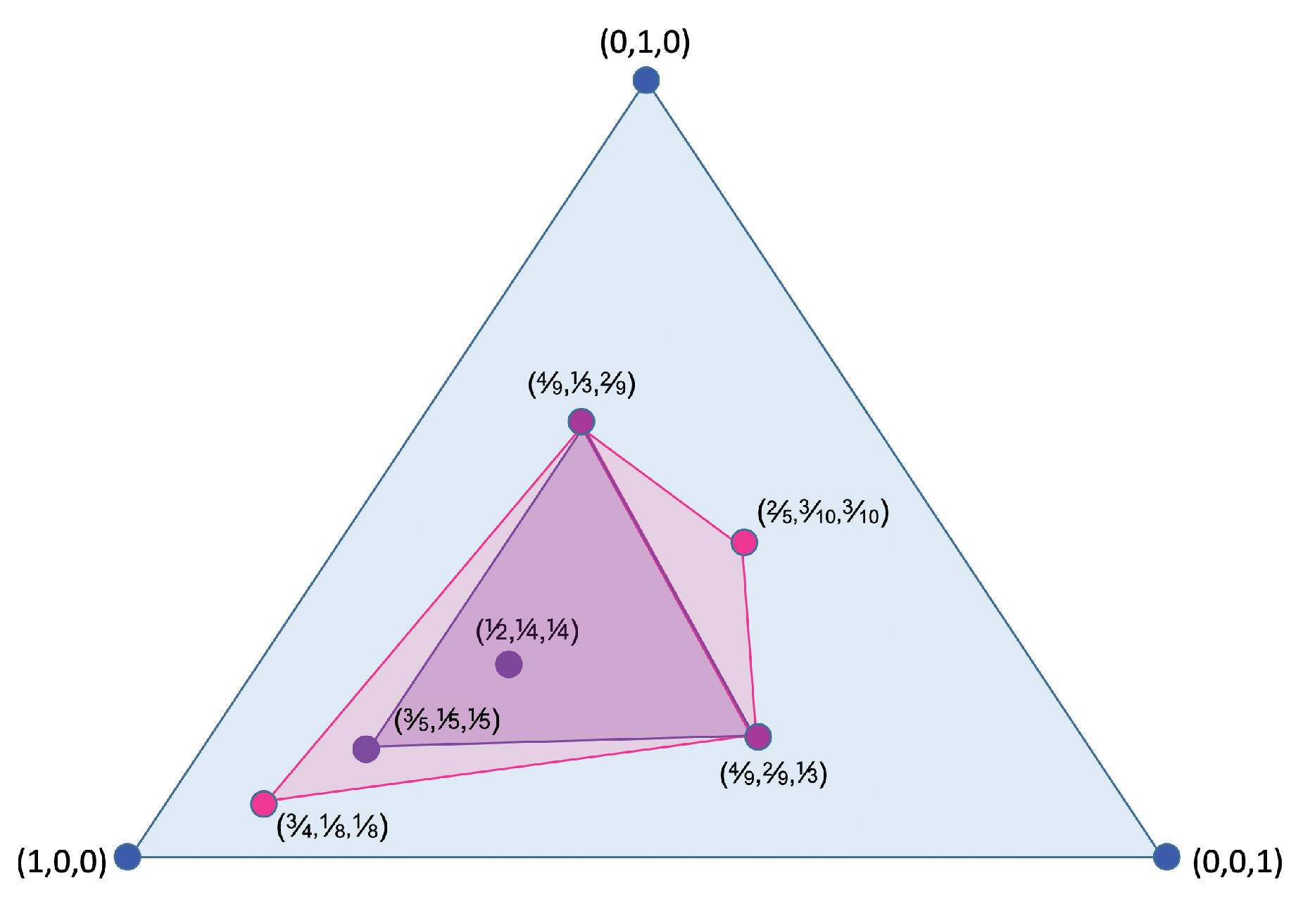
Theorem A1 has a nice geometric intuition (cf. Figure 2) that we are going to illustrate in the following example.

Figure 2. The simplex and the convex hulls of the posterior distributions in Example 5.

Example 5.

Consider the following systems.

$$\begin{array}{|ccccc|}\hline A& y_1& y_2& y_3& y_4\\ x_1& \raisebox{1ex}{$1$}\!\left/ \!\raisebox{-1ex}{$3$}\right.& \raisebox{1ex}{$2$}\!\left/ \!\raisebox{-1ex}{$9$}\right.& \raisebox{1ex}{$2$}\!\left/ \!\raisebox{-1ex}{$9$}\right.& \raisebox{1ex}{$2$}\!\left/ \!\raisebox{-1ex}{$9$}\right.\\ x_2& \raisebox{1ex}{$1$}\!\left/ \!\raisebox{-1ex}{$9$}\right.& \raisebox{1ex}{$1$}\!\left/ \!\raisebox{-1ex}{$3$}\right.& \raisebox{1ex}{$2$}\!\left/ \!\raisebox{-1ex}{$9$}\right.& \raisebox{1ex}{$1$}\!\left/ \!\raisebox{-1ex}{$3$}\right.\\ x_3& \raisebox{1ex}{$1$}\!\left/ \!\raisebox{-1ex}{$9$}\right.& \raisebox{1ex}{$2$}\!\left/ \!\raisebox{-1ex}{$9$}\right.& \raisebox{1ex}{$1$}\!\left/ \!\raisebox{-1ex}{$3$}\right.& \raisebox{1ex}{$1$}\!\left/ \!\raisebox{-1ex}{$3$}\right.\\ \hline\end{array}\begin{array}{|ccccc|}\hline B& y_1& y_2& y_3& y_4\\ x_1& \raisebox{1ex}{$1$}\!\left/ \!\raisebox{-1ex}{$3$}\right.& \raisebox{1ex}{$2$}\!\left/ \!\raisebox{-1ex}{$9$}\right.& \raisebox{1ex}{$2$}\!\left/ \!\raisebox{-1ex}{$9$}\right.& \raisebox{1ex}{$1$}\!\left/ \!\raisebox{-1ex}{$9$}\right.\\ x_2& \raisebox{1ex}{$2$}\!\left/ \!\raisebox{-1ex}{$9$}\right.& \raisebox{1ex}{$1$}\!\left/ \!\raisebox{-1ex}{$3$}\right.& \raisebox{1ex}{$2$}\!\left/ \!\raisebox{-1ex}{$9$}\right.& \raisebox{1ex}{$1$}\!\left/ \!\raisebox{-1ex}{$9$}\right.\\ x_3& \raisebox{1ex}{$2$}\!\left/ \!\raisebox{-1ex}{$9$}\right.& \raisebox{1ex}{$2$}\!\left/ \!\raisebox{-1ex}{$9$}\right.& \raisebox{1ex}{$1$}\!\left/ \!\raisebox{-1ex}{$3$}\right.& \raisebox{1ex}{$1$}\!\left/ \!\raisebox{-1ex}{$9$}\right.\\ \hline\end{array}$$

(11)

Consider the prior $\pi =(\raisebox{1ex}{$1$}\!\left/ \!\raisebox{-1ex}{$2$}\right.,\raisebox{1ex}{$1$}\!\left/ \!\raisebox{-1ex}{$4$}\right.,\raisebox{1ex}{$1$}\!\left/ \!\raisebox{-1ex}{$4$}\right.)$. The set of the posterior distributions generated by A under π are:

$$\mathit{supp}[\pi ,A]=\{(\raisebox{1ex}{$3$}\!\left/ \!\raisebox{-1ex}{$4$}\right.,\raisebox{1ex}{$1$}\!\left/ \!\raisebox{-1ex}{$8$}\right.,\raisebox{1ex}{$1$}\!\left/ \!\raisebox{-1ex}{$8$}\right.),(\raisebox{1ex}{$4$}\!\left/ \!\raisebox{-1ex}{$9$}\right.,\raisebox{1ex}{$1$}\!\left/ \!\raisebox{-1ex}{$3$}\right.,\raisebox{1ex}{$2$}\!\left/ \!\raisebox{-1ex}{$9$}\right.),(\raisebox{1ex}{$4$}\!\left/ \!\raisebox{-1ex}{$9$}\right.,\raisebox{1ex}{$2$}\!\left/ \!\raisebox{-1ex}{$9$}\right.,\raisebox{1ex}{$1$}\!\left/ \!\raisebox{-1ex}{$3$}\right.),(\raisebox{1ex}{$2$}\!\left/ \!\raisebox{-1ex}{$5$}\right.,\raisebox{1ex}{$3$}\!\left/ \!\raisebox{-1ex}{$10$}\right.,\raisebox{1ex}{$3$}\!\left/ \!\raisebox{-1ex}{$10$}\right.)\}$$

(12)

while those generated by B are:

$$\mathit{supp}[\pi ,B]=\{(\raisebox{1ex}{$3$}\!\left/ \!\raisebox{-1ex}{$5$}\right.,\raisebox{1ex}{$1$}\!\left/ \!\raisebox{-1ex}{$5$}\right.,\raisebox{1ex}{$1$}\!\left/ \!\raisebox{-1ex}{$5$}\right.),(\raisebox{1ex}{$4$}\!\left/ \!\raisebox{-1ex}{$9$}\right.,\raisebox{1ex}{$1$}\!\left/ \!\raisebox{-1ex}{$3$}\right.,\raisebox{1ex}{$2$}\!\left/ \!\raisebox{-1ex}{$9$}\right.),(\raisebox{1ex}{$4$}\!\left/ \!\raisebox{-1ex}{$9$}\right.,\raisebox{1ex}{$2$}\!\left/ \!\raisebox{-1ex}{$9$}\right.,\raisebox{1ex}{$1$}\!\left/ \!\raisebox{-1ex}{$3$}\right.),(\raisebox{1ex}{$1$}\!\left/ \!\raisebox{-1ex}{$2$}\right.,\raisebox{1ex}{$1$}\!\left/ \!\raisebox{-1ex}{$4$}\right.,\raisebox{1ex}{$1$}\!\left/ \!\raisebox{-1ex}{$4$}\right.)\}$$

(13)

These posteriors, and the convex hulls that they generate, are illustrated in Figure 2. The pink area is the ch supp$[\pi ,A]$ and the purple area is the ch supp$[\pi ,B]$. We can see that supp$[\pi ,B]\subseteq$ch supp$[\pi ,A]$, or, equivalently, ch supp$[\pi ,B]\subseteq$ch supp$[\pi ,A]$.

We are now ready to give the main result of this section.

Theorem 2.

The orders${⊑}^{\max }$and${⊑}_{\mathbb{Q}}^{\max }$coincide.

Similarly to the average case, $A{⊑}^{\max }B$ gives us a strong leakage guarantee: can safely replace A by B, knowing that, for any adversary, the max-case leakage of B can be no-larger than that of A. Moreover, in case $A{/⊑}^{\max }B$, we can always find an adversary, modelled by a vulnerability function V, who prefers (wrt the max-case) interacting with A that with B. Such a function is discussed in Section 5.

Finally, we resolve the question of how ${⊑}^{\max }$ and ${⊑}^{\mathrm{avg}}$ are related.

Theorem 3.

${⊑}^{\mathrm{avg}}$is strictly stronger than${⊑}^{\max }$.

This result might appear counter-intuitive at first; one might expect $A{⊑}^{\max }B$ to imply $A{⊑}^{\mathrm{avg}}B$. To understand why it does not, note that the former only requires that, for each output $y_B$ of B, there exists some output of $y_A$ that is at least as vulnerable, regardless of how likely $y_A$ and $y_B$ are to happen (this is max-case, after all). We illustrate this with the following example.

Example 6.

Consider the following systems:

$$\begin{array}{|ccccc|}\hline A& y_1& y_2& y_3& y_4\\ x_1& \raisebox{1ex}{$3$}\!\left/ \!\raisebox{-1ex}{$4$}\right.& 0& \raisebox{1ex}{$1$}\!\left/ \!\raisebox{-1ex}{$4$}\right.& 0\\ x_2& \raisebox{1ex}{$3$}\!\left/ \!\raisebox{-1ex}{$4$}\right.& \raisebox{1ex}{$1$}\!\left/ \!\raisebox{-1ex}{$4$}\right.& 0& 0\\ x_3& 0& \raisebox{1ex}{$1$}\!\left/ \!\raisebox{-1ex}{$4$}\right.& \raisebox{1ex}{$1$}\!\left/ \!\raisebox{-1ex}{$4$}\right.& \raisebox{1ex}{$1$}\!\left/ \!\raisebox{-1ex}{$2$}\right.\\ \hline\end{array}\begin{array}{|cccc|}\hline B& y_1& y_2& y_3\\ x_1& \raisebox{1ex}{$1$}\!\left/ \!\raisebox{-1ex}{$2$}\right.& 0& \raisebox{1ex}{$1$}\!\left/ \!\raisebox{-1ex}{$2$}\right.\\ x_2& \raisebox{1ex}{$1$}\!\left/ \!\raisebox{-1ex}{$2$}\right.& \raisebox{1ex}{$1$}\!\left/ \!\raisebox{-1ex}{$2$}\right.& 0\\ x_3& 0& \raisebox{1ex}{$1$}\!\left/ \!\raisebox{-1ex}{$2$}\right.& \raisebox{1ex}{$1$}\!\left/ \!\raisebox{-1ex}{$2$}\right.\\ \hline\end{array}$$

(14)

Under the uniform prior, the $y_1,y_2,y_3$ posteriors for both channels are the same, namely $(\raisebox{1ex}{$1$}\!\left/ \!\raisebox{-1ex}{$2$}\right.,\raisebox{1ex}{$1$}\!\left/ \!\raisebox{-1ex}{$2$}\right.,0)$, $(0,\raisebox{1ex}{$1$}\!\left/ \!\raisebox{-1ex}{$2$}\right.,\raisebox{1ex}{$1$}\!\left/ \!\raisebox{-1ex}{$2$}\right.)$ and $(\raisebox{1ex}{$1$}\!\left/ \!\raisebox{-1ex}{$2$}\right.,0,\raisebox{1ex}{$1$}\!\left/ \!\raisebox{-1ex}{$2$}\right.)$, respectively. Thus, the knowledge that can be obtained by each output of B can be also obtained by some output of A (albeit with a different probability). Hence, from Theorem A1, we get that $A{⊑}^{\max }B$. However, we can check (see Section 5.1) that B cannot be obtained by post-processing A, that is, $A{/⊑}^{\mathrm{avg}}B$.

The other direction might also appear tricky: if B leaks no more than A in the average-case, it must also leak no more than B in the max-case. The quantification over all gain functions in the average-case is powerful enough to “detect” differences in max-case leakage. The above result also means that ${⊑}^{\mathrm{avg}}$ could be useful even if we are interested in the max-case, since it gives us ${⊑}^{\max }$ for free.

4. Privacy-Based Refinement

Thus far, we have compared systems based on their (average-case or max-case) leakage. In this section, we turn our attention to the model of differential privacy and discuss new ways of ordering mechanisms based on that model.

4.1. Differential Privacy and $\mathit{d}$-Privacy

Differential privacy relies on the observation that some pairs of secrets need to be indistinguishable from the point of view of the adversary in order to provide some meaningful notion of privacy; for instance, databases differing in a single individual should not be distinguishable, otherwise the privacy of that individual is violated. At the same, other pairs of secrets can be allowed to be distinguishable in order to provide some utility; for instance, distinguishing databases differing in many individuals allows us to answer a statistical query about those individuals.

This idea can be formalized by a distinguishability metric $\mathit{d}$. (To be precise, $\mathit{d}$ is an extended pseudo metric, namely one in which distinct secrets can have distance 0, and distance $+\infty$ is allowed.) Intuitively, $\mathit{d}(x,x^{\prime })$ models how distinguishable we allow these secrets to be. A value 0 means that we require x and $x^{\prime }$ to be completely indistinguishable to the adversary, while $+\infty$ means that she can distinguish them completely.

In this context, a mechanism is simply a channel (the two terms will be used interchangeably), mapping secrets $\mathcal{X}$ to some observations $\mathcal{Y}$. Denote by $\mathbb{M}\mathcal{X}$ the set of all metrics on $\mathcal{X}$. Given $\mathit{d}\in \mathbb{M}\mathcal{X}$, we define $\mathit{d}$-privacy as follows:

Definition 3.

A channel C satisfies $\mathit{d}$-privacy iff

$$C_{x,y}\le e^{\mathit{d}(x,x^{\prime })}{C}_{x^{\prime },y}\mathrm{for}\mathrm{all}x,x^{\prime }\in \mathcal{X},y\in \mathcal{Y}$$

(15)

Intuitively, this definition requires that the closer x and $x^{\prime }$ are (as measured by $\mathit{d}$), the more similar (probabilistically) the output of the mechanism on these secrets should be.

Remark 1.

Note that the definition of $\mathit{d}$-privacy given in (1) is slightly different from the above one because of the presence of ε in the exponent. Indeed, it is common to scale $\mathit{d}$ by a privacy parameter $\epsilon \ge 0$, in which case $\mathit{d}$ can be thought of as the “kind” and ε as the “amount” of privacy. In other words, the structure determined by $\mathit{d}$ on the data specifies how we want to distinguish each pair of data, and ε specifies (uniformly) the degree of the distinction. Note that $\epsilon ·\mathit{d}$ is itself a metric, so the two definitions are equivalent.

Using a generic metric $\mathit{d}$ in this definition allows us to express different scenarios, depending on the domain $\mathcal{X}$ on which the mechanism is applied and the choice of $\mathit{d}$. For instance, in the standard model of differential privacy, the mechanism is applied to a database x (i.e., $\mathcal{X}$ is the set of all databases), and produces some observation y (e.g., a number). The Hamming metric ${\mathit{d}}_{\mathrm{H}}$—defined as the number of individuals in which x and $x^{\prime }$ differ—captures standard differential privacy.

4.2. Oblivious Mechanisms

In the case of an oblivious mechanism, a query $f:\mathcal{X}\to \mathcal{Y}$ is first applied to database x, and a noise mechanism H from $\mathcal{Y}$ to $\mathcal{Z}$ is applied to $y=f\left(x\right)$, producing an observation z. In this case, it is useful to study the privacy of H wrt some metric ${\mathit{d}}_{\mathcal{Y}}$ on $\mathcal{Y}$. Then, to reason about the ${\mathit{d}}_{\mathcal{X}}$-privacy of the whole mechanism $H\circ f$, we can first compute the sensitivity of f wrt ${\mathit{d}}_{\mathcal{X}},{\mathit{d}}_{\mathcal{Y}}$:

$${\Delta }_{{\mathit{d}}_{\mathcal{X}},{\mathit{d}}_{\mathcal{Y}}}^f=\underset{x,x^{\prime }}{\max }\frac{{\mathit{d}}_{\mathcal{Y}}(f\left(x\right),f\left(x^{\prime }\right))}{{\mathit{d}}_{\mathcal{X}}(x,x^{\prime })}$$

(16)

and then use the following property [3]:

$$\begin{array}{c}\hfill \mathrm{If}H\mathrm{satisfies}{\mathit{d}}_{\mathcal{Y}}-\mathrm{privacy},\mathrm{then}H\circ f\mathrm{satisfies}{\Delta }_{{\mathit{d}}_{\mathcal{X}},{\mathit{d}}_{\mathcal{Y}}}^f·{\mathit{d}}_{\mathcal{X}}-\mathrm{privacy}.\end{array}$$

(17)

For instance, the geometric mechanism $G^{\epsilon }$ satisfies $\epsilon ·{\mathit{d}}_{\mathrm{E}}$-privacy (where ${\mathit{d}}_{\mathrm{E}}$ denotes the Euclidean metric), hence it can be applied to any numeric query f: the resulting mechanism $G^{\epsilon }\circ f$ satisfies ${\Delta }_{{\mathit{d}}_{\mathrm{H}},{\mathit{d}}_{\mathrm{E}}}^f·\epsilon$-differential privacy. The sensitivity wrt the Hamming and Euclidean metrics reduces to ${\Delta }_{{\mathit{d}}_{\mathrm{H}},{\mathit{d}}_{\mathrm{E}}}^f={\max }_{x\sim x^{\prime }}|f\left(x\right)-f\left(x^{\prime }\right)|$ where $x\sim x^{\prime }$ denotes ${\mathit{d}}_{\mathrm{H}}(x,x^{\prime })=1$.

4.3. Applying Noise to the Data of a Single Individual

There are also scenarios in which a mechanism C is applied directly to the data of a single individual (that is, $\mathcal{X}$ is the set of possible values). For instance, in the local model of differential privacy [2], the value of each individual is obfuscated before sending them to an untrusted curator. In this case, C should satisfy ${\mathit{d}}_{\mathrm{D}}$-privacy, where ${\mathit{d}}_{\mathrm{D}}$ is the discrete metric, since any change in the individual’s value should have negligible effects.

Moreover, in the context of location-based services, a user might want to obfuscate his location before sending it to the service provider. In this context, it is natural to require that locations that are geographically close are indistinguishable, while far away ones are allowed to be distinguished (in order to provide the service). In other words, we wish to provide ${\mathit{d}}_{\mathrm{E}}$-privacy, for the Euclidean metric on ${\mathbb{R}}^2$, called geo-indistinguishability in [17].

4.4. Comparing Mechanisms by Their “Smallest $\epsilon$” (For Fixed $\mathit{d}$)

Scaling $\mathit{d}$ by a privacy parameter $\epsilon$ allows us to turn $\mathit{d}$-privacy (for some fixed $\mathit{d}$) into a quantitative “leakage” measure, by associating each channel to the smallest ε by which we can scale $\mathit{d}$ without violating privacy.

Definition 4.

The privacy-based leakage (wrt $\mathit{d}$) of a channel C is defined as

$${\mathrm{Priv}}_{\mathit{d}}\left(C\right):=\inf \{\epsilon \ge 0|C\mathrm{satisfies}\epsilon ·\mathit{d}-\mathrm{privacy}\}$$

(18)

Note that ${\mathrm{Priv}}_{\mathit{d}}\left(C\right)=+\infty$ iff there is no such $\epsilon$; also ${\mathrm{Priv}}_{\mathit{d}}\left(C\right)\le 1$ iff C satisfies $\mathit{d}$-privacy.

It is then natural to compare two mechanisms A and B based on their “smallest $\epsilon$”.

Definition 5.

Define $A{⊑}_{\mathit{d}}^{\mathrm{prv}}B$ iff ${\mathrm{Priv}}_{\mathit{d}}\left(A\right)\ge {\mathrm{Priv}}_{\mathit{d}}\left(B\right)$.

For instance, $A{⊑}_{{\mathit{d}}_{\mathrm{H}}}^{\mathrm{prv}}B$ means that B satisfies standard differential privacy for $\epsilon$ at least as small as the one of A.

4.5. Privacy-Based Leakage and Refinement Orders

When discussing the average- and max-case leakage orders ${⊑}_{\mathbb{G}}^{\mathrm{avg}},{⊑}_{\mathbb{Q}}^{\max }$, we obtained strong leakage guarantees by quantifying over all vulnerability functions. It is thus natural to investigate a similar quantification in the context of $\mathit{d}$-privacy. Namely, we define a stronger privacy-based “leakage” order, by comparing mechanisms not on a single metric $\mathit{d}$, but on all metrics simultaneously.

Definition 6.

The privacy-based leakage order is defined as $A{⊑}_{\mathbb{M}}^{\mathrm{prv}}B$ iff $A{⊑}_{\mathit{d}}^{\mathrm{prv}}B$ for all $\mathit{d}\in \mathbb{M}\mathcal{X}$.

Similarly to the other leakage orders, the drawback of ${⊑}_{\mathbb{M}}^{\mathrm{prv}}$ is that it quantifies over an uncountable family of metrics. As a consequence, our first goal is to characterize it as a property of the channel matrix alone, which would make it much easier to reason about or verify.

To do so, we start by recalling an alternative way of thinking about $\mathit{d}$-privacy. Consider the multiplicative total variation distance between probability distributions $\mu ,{\mu }^{\prime }\in \mathbb{D}\mathcal{Y}$, defined as:

$${\mathrm{tv}}_{\otimes }(\mu ,{\mu }^{\prime }):=\underset{y:\mathcal{Y}}{\max }|\ln \frac{{\mu }_y}{{\mu }_y^{\prime }}|$$

(19)

If we think of C as a function $\mathcal{X}\to \mathbb{D}\mathcal{Y}$ (mapping every x to the distribution $C_{x,-}$), C satisfies $\mathit{d}$-privacy iff ${\mathrm{tv}}_{\otimes }(C_{x,-},C_{x^{\prime },-})\le \mathit{d}(x,x^{\prime })$, in other words iff C is non-expansive (1-Lipschitz) wrt ${\mathrm{tv}}_{\otimes },\mathit{d}$.

Then, we introduce the concept of the distinguishability metric ${\mathit{d}}_C\in \mathbb{M}\mathcal{X}$ induced by the channel C, defined as

$${\mathit{d}}_C(x,x^{\prime }):={\mathrm{tv}}_{\otimes }(C_{x,-},C_{x^{\prime },-})$$

(20)

Intuitively, ${\mathit{d}}_C(x,x^{\prime })$ expresses exactly how much the channel distinguishes (wrt ${\mathrm{tv}}_{\otimes }$) the secrets $x,x^{\prime }$. It is easy to see that ${\mathit{d}}_C$ is the smallest metric for which C is private; in other words, for any $\mathit{d}$:

$$C\mathrm{satisfies}\mathit{d}-\mathrm{privacy}\mathrm{iff}\mathit{d}\ge {\mathit{d}}_C$$

(21)

We can now give a refinement order on mechanisms, by comparing their corresponding induced metrics.

Definition 7.

The privacy-based refinement order is defined as $A{⊑}^{\mathrm{prv}}B$ iff ${\mathit{d}}_A\ge {\mathit{d}}_B$, or equivalently iff B satisfies ${\mathit{d}}_A$-privacy.

This achieves our goal of goal of characterizing ${⊑}_{\mathbb{M}}^{\mathrm{prv}}$.

Proposition 1.

The orders${⊑}_{\mathbb{M}}^{\mathrm{prv}}$and${⊑}^{\mathrm{prv}}$coincide.

We now turn our attention to the question of how these orders relate to each other.

Theorem 4.

${⊑}^{\max }$is strictly stronger than${⊑}^{\mathrm{prv}}$, which is strictly stronger than${⊑}_{\mathit{d}}^{\mathrm{prv}}$.

The fact that ${⊑}^{\max }$ is stronger than ${⊑}^{\mathrm{prv}}$ is due to the fact than ${\mathrm{Priv}}_{\mathit{d}}$ can be seen as a max-case information leakage, for a properly constructed vulnerability function $V_{\mathit{d}}$. This is discussed in detail in Section 4.7. This implication means that ${⊑}^{\mathrm{avg}},{⊑}^{\max }$ can be useful even if we “only” care about $\mathit{d}$-privacy.

4.6. Application to Oblivious Mechanisms

We conclude the discussion on privacy-based refinement by showing the usefulness of our strong ${⊑}^{\mathrm{prv}}$ order in the case of oblivious mechanisms.

Theorem 5.

Let $f:\mathcal{X}\to \mathcal{Y}$ be any query and $A,B$ be two mechanisms on $\mathcal{Y}$. If $A{⊑}^{\mathrm{prv}}B$, then $A\circ f{⊑}^{\mathrm{prv}}B\circ f$.

This means that replacing A by B is the context of an oblivious mechanism is always safe, regardless of the query (and its sensitivity) and regardless of the metric by which the privacy of the composed mechanism is evaluated.

Assume, for instance that we care about standard differential privacy, and we have properly constructed A such that $A\circ f$ satisfies $\epsilon$-differential privacy for some $\epsilon$. If we know that $A{⊑}^{\mathrm{prv}}B$ (several such cases are discussed in Section 6), we can replace A by B without even knowing what f does. The mechanism $B\circ f$ is guaranteed to also satisfy $\epsilon$-differential privacy.

Note also that the above theorem fails for the weaker order ${⊑}_{\mathit{d}}^{\mathrm{prv}}$. Establishing $A{⊑}_{{\mathit{d}}_{\mathcal{Y}}}^{\mathrm{prv}}B$ for some metric ${\mathit{d}}_{\mathcal{Y}}:\mathbb{M}\mathcal{Y}$ gives no guarantees that $A\circ f{⊑}_{{\mathit{d}}_{\mathcal{X}}}^{\mathrm{prv}}B\circ f$ for some other metric of interest ${\mathit{d}}_{\mathcal{X}}:\mathbb{M}\mathcal{X}$. It is possible that replacing A by B in that case is not safe (one would need to re-examine the behavior of B, and possibly reconfigure it to the sensitivity of f).

Table 3 summarizes the relations between the various orderings.

Table 3. Comparison of leakage and refinement orders. All implications are strict.

Leakage Orders		Refinement Orders
${⊑}_{\mathbb{G}}^{\mathrm{avg}}$	⇔	${⊑}^{\mathrm{avg}}$
⇓		⇓
${⊑}_{\mathbb{Q}}^{\max }$	⇔	${⊑}^{\max }$
⇓		⇓
${⊑}_{\mathbb{M}}^{\mathrm{prv}}$	⇔	${⊑}^{\mathrm{prv}}$
⇘		⇙
	${⊑}_{\mathit{d}}^{\mathrm{prv}}$

4.7. Privacy as Max-Case Capacity

In this section we show that $\mathit{d}$-privacy can be expressed as a (max-case) information leakage. Note that this provides an alternative proof that ${⊑}^{\max }$ is stronger than ${⊑}^{\mathrm{prv}}$. We start this by defining a suitable vulnerability function:

Definition 8.

The $\mathit{d}$-vulnerability function $V_{\mathit{d}}$ is defined as

$$V_{\mathit{d}}\left(\pi \right):=\inf \{\epsilon \ge 0|\forall x,x^{\prime }\in \mathcal{X},{\pi }_x\le e^{\epsilon ·\mathit{d}(x,x^{\prime })}{\pi }_{x^{\prime }}\}$$

(22)

Note the difference between $V_{\mathit{d}}\left(\pi \right)$ (a vulnerability function on distributions) and ${\mathrm{Priv}}_{\mathit{d}}\left(C\right)$ (a “leakage” measure on channels).

A fundamental notion in QIF is that of capacity: the maximization of leakage over all priors. In turns out that, for $V_{\mathit{d}}$, the capacity-realizing prior is the uniform one. In the following, ${\mathcal{L}}_{\mathit{d}}^{+,\max }$ denotes the additive max-case $\mathit{d}$ leakage, namely:

$${\mathcal{L}}_{\mathit{d}}^{+,\max }(\pi ,C)=V_{\mathit{d}}^{\max }[\pi ,C]-V_{\mathit{d}}\left(\pi \right)$$

(23)

and $\mathcal{M}{\mathcal{L}}_{\mathit{d}}^{+,\max }$ denotes the additive max-case $\mathit{d}$-capacity, namely:

$$\mathcal{M}{\mathcal{L}}_{\mathit{d}}^{+,\max }\left(C\right)=\underset{\pi }{\max }{\mathcal{L}}_{\mathit{d}}^{+,\max }(\pi ,C)$$

(24)

Theorem 6.

$\mathcal{M}{\mathcal{L}}_{\mathit{d}}^{+,\max }$is always achieved on a uniform prior${\pi }^u$. Namely

$$\underset{\pi }{\max }{\mathcal{L}}_{\mathit{d}}^{+,\max }(\pi ,C)={\mathcal{L}}_{\mathit{d}}^{+,\max }({\pi }^u,C)=V_{\mathit{d}}^{\max }[{\pi }^u,C]$$

(25)

This finally brings us to our goal of expressing ${\mathrm{Priv}}_{\mathit{d}}$ in terms of information leakage (for a proper vulnerability function).

Theorem 7.

[DP as max-case capacity] C satisfies $\epsilon ·\mathit{d}$-privacy iff $\mathcal{M}{\mathcal{L}}_{\mathit{d}}^{+,\max }\left(C\right)\le \epsilon$. In other words: $\mathcal{M}{\mathcal{L}}_{\mathit{d}}^{+,\max }\left(C\right)={\mathrm{Priv}}_{\mathit{d}}\left(C\right)$.

5. Verifying the Refinement Orders

We now turn our attention to the problem of checking whether the various orders hold, given two explicit representations of channels A and B (in terms of their matrices). We show that, for all orders, this question can be answered in time polynomial in the size of the matrices. Moreover, when one of the order fails, we discuss how to obtain a counter-example (e.g., a gain function g or a vulnerability function V), demonstrating this fact. All the methods discussed in the section have been implemented in a publicly available library, and have been used in the experimental results of Section 6.

5.1. Average-Case Refinement

Verifying $A{⊑}^{\mathrm{avg}}B$ can be done in polynomial time (in the size of $A,B$) by solving the system of equations $AR=B$, with variables R, under the linear constraints that R is a channel matrix (non-negative and rows sum up to 1). However, if the system has no solution (i.e., $A{/⊑}^{\mathrm{avg}}B$), this method does not provide us with a counter-example gain function g.

We now show that there is an alternative efficient method: define $C^{\uparrow }=\left\{CR\right|R\mathrm{is}\mathrm{a}\mathrm{channel}\}$, the set of all channels obtainable by post-processing C. The idea is to compute the projection of B on $A^{\uparrow }$. Clearly, the projection is B itself iff $A{⊑}^{\mathrm{avg}}B$; otherwise, the projection can be directly used to construct a counter-example g.

Theorem 8.

Let$B^{*}$be the projection ofBon$A^{\uparrow }$.

1. 

If $B=B^{*}$, then $A{⊑}^{\mathrm{avg}}B$.

2. 

Otherwise, let $G=B-B^{*}$. The gain function $g(w,x)=G_{x,w}$ provides a counter-example to $A{⊑}^{\mathrm{avg}}B$, which is $V_g({\pi }^u,A)<V_g({\pi }^u,B)$, for uniform ${\pi }^u$.

Since ${\parallel x-y\parallel }_2^2=x^{T}x-2x^{T}y+y^{T}y$, the projection of y to a convex set can be written as ${\min }_x{x}^{T}x-2x^{T}y$ for $Ax\le b$. This is a quadratic program with Q being the identity matrix, which is positive definite, hence it can be solved in polynomial time.

Note that the proof that ${⊑}_{\mathbb{G}}^{\mathrm{avg}}$ is stronger than ${⊑}^{\mathrm{avg}}$ (the “coriaceous” theorem of [7]) uses the hyperplane-separation theorem to show the existence of a counter example g in case $A{/⊑}^{\mathrm{avg}}B$. The above technique essentially computes such a separating hyperplane.

5.2. Max-Case Refinement

Similarly to ${⊑}^{\mathrm{avg}}$, we can verify $A{⊑}^{\max }B$ directly using its definition, by solving the system $R\tilde{A}=\tilde{B}$ under the constraint that R is a channel.

In contrast to ${⊑}^{\mathrm{avg}}$, when $A{/⊑}^{\max }B$, the proof of Theorem 2 directly gives us a counter-example:

$$V\left(\sigma \right):=\underset{{\sigma }^{\prime }:S}{\min }{\parallel \sigma -{\sigma }^{\prime }\parallel }_2$$

(26)

where $S=$ ch supp $[\pi ,A]$ and $\pi$ is any full-support prior. For this vulnerability function, it holds that $V^{\max }(\pi ,A)<V^{\max }(\pi ,B)$.

5.3. Privacy-Based Refinement

The ${⊑}^{\mathrm{prv}}$ order can be verified directly from its definition, by checking that ${\mathit{d}}_A\ge {\mathit{d}}_B$. This can be done in time $O\left(\right|\mathcal{X}{|}^2\left|\mathcal{Y}\right|)$, by computing ${\mathrm{tv}}_{\otimes }(C_{x,-},C_{x^{\prime },-})$ for each pair of secrets. If $A{/⊑}^{\mathrm{prv}}B$, then $\mathit{d}={\mathit{d}}_B$ provides an immediate counter-example metric, since B satisfies ${\mathit{d}}_B$-privacy, but A does not.

6. Application: Comparing DP Mechanisms

In differential privacy, it is common to compare the privacy guarantees provided by different mechanisms by ‘comparing the epsilons’. However, it is interesting to ask to what extent $\epsilon$-equivalent mechanisms are comparable wrt the other leakage measures defined here—or we might want to know whether reducing $\epsilon$ in a mechanism also corresponds to a refinement of it. This could be useful if, for example, it is important to understand the privacy properties of a mechanism with respect to any max-case leakage measure, and not just the DP measure given by $\epsilon$.

Since the $\epsilon$-based order given by ${⊑}_{\mathit{d}}^{\mathrm{prv}}$ is (strictly) the weakest of the orders considered here, it cannot be the case that we always get a refinement (wrt other orders). However, it may be true that, for particular families of mechanisms, some (or all) of the refinement orders hold.

We investigate three families of mechanisms commonly used in DP or LDP: geometric, exponential and randomized response mechanisms.

6.1. Preliminaries

We define each family of mechanisms in terms of their channel construction. We assume that mechanisms operate on a set of inputs (denoted by $\mathcal{X}$) and produce a set of outputs (denoted $\mathcal{Y}$). In this sense, our mechanisms can be seen as oblivious (as in standard DP) or as LDP mechanisms. (We use the term ‘mechanism’ in either sense). We denote by $M^{\epsilon }$ a mechanism parametrized by $\epsilon$, where $\epsilon$ is defined to be the same as ${\mathrm{Priv}}_{\mathit{d}}\left(M\right)$. For the purposes of comparison, we make sure that we use the best possible $\epsilon$ for each mechanism. In order to compare mechanisms, we restrict our input and output domains of interest to sequences of non-negative integers. We assume $\mathcal{X},\mathcal{Y}$ are finite unless specified. In addition, as we are operating in the framework of $\mathit{d}$-privacy, it is necessary to provide an appropriate metric defined over $\mathcal{X}$; here, it makes sense to use the Euclidean distance metric ${\mathit{d}}_{\mathrm{E}}$.

Definition 9.

A geometric mechanism is a channel $(\mathcal{X},\mathbb{Z},G^{\epsilon })$, parametrized by $\epsilon \ge 0$ constructed as follows:

$$\begin{array}{ccc}\hfill G_{x,y}^{\epsilon }& =\frac{(1-\alpha )·{\alpha }^{{\mathit{d}}_{\mathrm{E}}(x,y)}}{1+\alpha }\hfill & \hfill \mathrm{for}\mathrm{all}x\in \mathcal{X},y\in \mathbb{Z}\end{array}$$

(27)

where $\alpha =e^{-\epsilon }$ and ${\mathit{d}}_{\mathrm{E}}(x,y)=\parallel x-y\parallel$. Such a mechanism satisfies $\epsilon ·{\mathit{d}}_{\mathrm{E}}$-privacy.

In practice, the truncated geometric mechanism is preferred to the infinite geometric. We define the truncated geometric mechanism as follows.

Definition 10.

A truncated geometric mechanism is a channel $(\mathcal{X},\mathcal{Y},T{G}^{\epsilon })$, parametrized by $\epsilon \ge 0$ with $\mathcal{X}\subseteq \mathcal{Y}$ constructed as follows:

$$\begin{array}{ccc}\hfill T{G}_{x,y}^{\epsilon }& =\frac{(1-\alpha )·{\alpha }^{{\mathit{d}}_{\mathrm{E}}(x,y)}}{1+\alpha }\hfill & \hfill \mathrm{for}\mathrm{all}y\ne \min \mathcal{Y},\max \mathcal{Y}\end{array}$$

(28)

$$\begin{array}{ccc}\hfill T{G}_{x,y}^{\epsilon }& =\frac{{\alpha }^{{\mathit{d}}_{\mathrm{E}}(x,y)}}{1+\alpha }\hfill & \hfill \mathrm{for}y=\min \mathcal{Y},\max \mathcal{Y}\end{array}$$

(29)

where $\alpha =e^{-\epsilon }$ and ${\mathit{d}}_{\mathrm{E}}(x,y)=\parallel x-y\parallel$. Such a mechanism satisfies $\epsilon ·{\mathit{d}}_{\mathrm{E}}$-privacy.

It is also possible to define the ‘over-truncated’ geometric mechanism whose input space is not entirely included in the output space.

Definition 11.

An over-truncated geometric mechanism is a channel $(\mathcal{X},\mathcal{Y},OT{G}^{\epsilon })$, parametrized by $\epsilon \ge 0$ with $\mathcal{X}/\subseteq \mathcal{Y}$ constructed as follows:

1. 

Start with the truncated geometric mechanism $(\mathcal{X},\mathcal{X}\cup \mathcal{Y},T{G}^{\epsilon })$.

2. 

Sum up the columns at each end until the output domain is reached.

Such a mechanism satisfies $\epsilon ·{\mathit{d}}_{\mathrm{E}}$-privacy.

For example, the set of inputs to an over-truncated geometric mechanism could be integers in the range $[0\dots 100]$, but the output space may have a range of $[0\dots 50]$ or perhaps $[-50\dots 50]$. In either of these cases, the mechanism has to ‘over-truncate’ the inputs to accommodate the output space.

We remark that we do not consider the over-truncated mechanism a particularly useful mechanism in practice. However, we provide results on this mechanism for completeness since its construction is possible, if unusual.

Definition 12.

An exponential mechanism is a channel $(\mathcal{X},\mathcal{Y},E^{\alpha })$, parametrized by $\epsilon \ge 0$ constructed as follows:

$$\begin{array}{ccc}\hfill E_{x,y}^{\alpha }& ={\lambda }_x·e^{-\frac{\epsilon }{2}{\mathit{d}}_{\mathrm{E}}(x,y)}\hfill & \hfill \mathrm{for}\mathrm{all}x\in \mathcal{X},y\in \mathcal{Y}\end{array}$$

(30)

where ${\lambda }_x$ are normalizing constants ensuring ${\sum }_y{E}_{x,y}^{\alpha }=1$. Such a mechanism satisfies $\alpha ·{\mathit{d}}_{\mathrm{E}}$-privacy where $\alpha \ge \frac{\epsilon }{2}$ (which can be calculated exactly from the channel construction).

Note that the construction presented in Definition 12 uses the Euclidean distance metric since we only consider integer domains. The general construction of the exponential mechanism uses arbitrary domains and arbitrary metrics. Note that its parameter $\epsilon$ does not correspond to the true (best-case) $\epsilon$-DP guarantee that it provides. We will denote by $E^{\epsilon }$ the exponential mechanism with ‘true’ privacy parameter $\epsilon$ rather than the reported one, as our intention is to capture the privacy guarantee provided by the channel in order to make reasonable comparisons.

Definition 13.

A randomized response mechanism is a channel $(\mathcal{X},\mathcal{Y},R^{\epsilon })$, parametrized by $\epsilon \ge 0$ constructed as follows:

$$\begin{array}{ccc}\hfill R_{x,y}^{\epsilon }& =\frac{e^{\epsilon (1-{\mathit{d}}_{\mathrm{D}}(x,y))}}{e^{\epsilon }+n}\hfill & \hfill \mathrm{for}\mathrm{all}x,y\in \mathcal{Y}\end{array}$$

(31)

$$\begin{array}{ccc}\hfill R_{x,y}^{\epsilon }& =\frac{1}{n+1}\hfill & \hfill \mathrm{for}\mathrm{all}x\notin \mathcal{Y}\end{array}$$

(32)

where $n=\parallel \mathcal{Y}\parallel -1$ and ${\mathit{d}}_{\mathrm{D}}$ is the discrete metric (that is, ${\mathit{d}}_{\mathrm{D}}(x,x)=0$ and ${\mathit{d}}_{\mathrm{D}}(x,y)=1$ for $x\in \mathcal{Y},x\ne y$). Such a mechanism satisfies $\epsilon ·{\mathit{d}}_{\mathrm{D}}$-privacy.

We note that the randomized response mechanism also satisfies $\epsilon ·{\mathit{d}}_{\mathrm{E}}$-privacy.

Intuitively, the randomized response mechanism returns the true answer with high probability and all other responses with equal probability. In the case where the input x lies outside $\mathcal{Y}$ (that is, in ‘over-truncated’ mechanisms), all of the outputs (corresponding to the outlying inputs) have equal probability.

Example 7.

The following are examples of each of the mechanisms described above, represented as channel matrices. For this example, we set $\epsilon =\log \left(2\right)$ for the geometric and randomized response mechanisms, while, for the exponential mechanism, we use $\epsilon =\log \left(4\right)$.

$$\begin{array}{cc}\hfill \begin{array}{|cccc|}\hline TG& x_1& x_2& x_3\\ x_1& \raisebox{1ex}{$2$}\!\left/ \!\raisebox{-1ex}{$3$}\right.& \raisebox{1ex}{$1$}\!\left/ \!\raisebox{-1ex}{$6$}\right.& \raisebox{1ex}{$1$}\!\left/ \!\raisebox{-1ex}{$6$}\right.\\ x_2& \raisebox{1ex}{$1$}\!\left/ \!\raisebox{-1ex}{$3$}\right.& \raisebox{1ex}{$1$}\!\left/ \!\raisebox{-1ex}{$3$}\right.& \raisebox{1ex}{$1$}\!\left/ \!\raisebox{-1ex}{$3$}\right.\\ x_3& \raisebox{1ex}{$1$}\!\left/ \!\raisebox{-1ex}{$6$}\right.& \raisebox{1ex}{$1$}\!\left/ \!\raisebox{-1ex}{$6$}\right.& \raisebox{1ex}{$2$}\!\left/ \!\raisebox{-1ex}{$3$}\right.\\ \hline\end{array}& \begin{array}{|ccc|}\hline OTG& x_1& x_2\\ x_1& \raisebox{1ex}{$2$}\!\left/ \!\raisebox{-1ex}{$3$}\right.& \raisebox{1ex}{$1$}\!\left/ \!\raisebox{-1ex}{$3$}\right.\\ x_2& \raisebox{1ex}{$1$}\!\left/ \!\raisebox{-1ex}{$3$}\right.& \raisebox{1ex}{$2$}\!\left/ \!\raisebox{-1ex}{$3$}\right.\\ x_3& \raisebox{1ex}{$1$}\!\left/ \!\raisebox{-1ex}{$6$}\right.& \raisebox{1ex}{$5$}\!\left/ \!\raisebox{-1ex}{$6$}\right.\\ \hline\end{array}\hfill \\ \hfill \\ \hfill \begin{array}{|cccc|}\hline E& x_1& x_2& x_3\\ x_1& \raisebox{1ex}{$4$}\!\left/ \!\raisebox{-1ex}{$7$}\right.& \raisebox{1ex}{$2$}\!\left/ \!\raisebox{-1ex}{$7$}\right.& \raisebox{1ex}{$1$}\!\left/ \!\raisebox{-1ex}{$7$}\right.\\ x_2& \raisebox{1ex}{$1$}\!\left/ \!\raisebox{-1ex}{$4$}\right.& \raisebox{1ex}{$1$}\!\left/ \!\raisebox{-1ex}{$2$}\right.& \raisebox{1ex}{$1$}\!\left/ \!\raisebox{-1ex}{$4$}\right.\\ x_3& \raisebox{1ex}{$1$}\!\left/ \!\raisebox{-1ex}{$7$}\right.& \raisebox{1ex}{$2$}\!\left/ \!\raisebox{-1ex}{$7$}\right.& \raisebox{1ex}{$4$}\!\left/ \!\raisebox{-1ex}{$7$}\right.\\ \hline\end{array}& \begin{array}{|cccc|}\hline R& x_1& x_2& x_3\\ x_1& \raisebox{1ex}{$1$}\!\left/ \!\raisebox{-1ex}{$2$}\right.& \raisebox{1ex}{$1$}\!\left/ \!\raisebox{-1ex}{$4$}\right.& \raisebox{1ex}{$1$}\!\left/ \!\raisebox{-1ex}{$4$}\right.\\ x_2& \raisebox{1ex}{$1$}\!\left/ \!\raisebox{-1ex}{$4$}\right.& \raisebox{1ex}{$1$}\!\left/ \!\raisebox{-1ex}{$2$}\right.& \raisebox{1ex}{$1$}\!\left/ \!\raisebox{-1ex}{$4$}\right.\\ x_3& \raisebox{1ex}{$1$}\!\left/ \!\raisebox{-1ex}{$4$}\right.& \raisebox{1ex}{$1$}\!\left/ \!\raisebox{-1ex}{$4$}\right.& \raisebox{1ex}{$1$}\!\left/ \!\raisebox{-1ex}{$2$}\right.\\ \hline\end{array}\hfill \end{array}$$

(33)

Note that the exponential mechanism here actually satisfies $\log \left(\frac{16}{7}\right)·{\mathit{d}}_{\mathrm{E}}$-privacy even though it is specified by $\epsilon =\log \left(4\right)$.

We now have three families of mechanisms which we can characterize by channels, and which satisfy $\epsilon ·{\mathit{d}}_{\mathrm{E}}$-privacy. For the remainder of this section, we will refer only to the $\epsilon$ parameter and take ${\mathit{d}}_{\mathrm{E}}$ as given, as we wish to understand the effect of changing $\epsilon$ (for a fixed metric) on the various leakage measures.

6.2. Refinement Order within Families of Mechanisms

We first ask which refinement orders hold within a family of mechanisms. That is, when does reducing $\epsilon$ for a particular mechanism produce a refinement? Since we have the convenient order ${⊑}^{\mathrm{avg}}\subset {⊑}^{\max }\subset {⊑}^{\mathrm{prv}}$, it is useful to first check if ${⊑}^{\mathrm{avg}}$ holds as we get the other refinements ‘for free’.

For the (infinite) geometric mechanism, we have the following result.

Theorem 9.

Let $G^{\epsilon },G^{{\epsilon }^{\prime }}$ be geometric mechanisms. Then, $G^{\epsilon }{⊑}^{\mathrm{avg}}{G}^{{\epsilon }^{\prime }}$ iff $\epsilon \ge {\epsilon }^{\prime }$. That is, decreasing $\epsilon$ produces a refinement of the mechanism.

This means that reducing $\epsilon$ in an infinite geometric mechanism is safe against any adversary that can be modelled using, for example, max-case or average-case vulnerabilities.

For the truncated geometric mechanism, we get the same result.

Theorem 10.

Let $T{G}^{\epsilon },T{G}^{{\epsilon }^{\prime }}$ be truncated geometric mechanisms. Then, $T{G}^{\epsilon }{⊑}^{\mathrm{avg}}T{G}^{{\epsilon }^{\prime }}$ iff $\epsilon \ge {\epsilon }^{\prime }$. That is, decreasing $\epsilon$ produces a refinement of the mechanism.

However, the over-truncated geometric mechanism does not behave so well.

Theorem 11.

Let $OT{G}^{\epsilon },OT{G}^{{\epsilon }^{\prime }}$ be over-truncated geometric mechanisms. Then, $OT{G}^{\epsilon }{/⊑}^{\mathrm{avg}}OT{G}^{{\epsilon }^{\prime }}$ for any $\epsilon \ne {\epsilon }^{\prime }$. That is, decreasing $\epsilon$ does not produce a refinement.

We can think of this last class of geometrics as ‘skinny’ mechanisms, that is, corresponding to a channel with a smaller output space than input space.

Intuitively, this theorem means that we can always find some (average-case) adversary who prefers the over-truncated geometric mechanism with the smaller $\epsilon$.

We remark that the gain function we found can be easily calculated by treating the columns of channel A as vectors, and finding a vector orthogonal to both of these. This follows from the results in Section 5.1. Since the columns of A cannot span the space ${\mathbb{R}}^3$, it is always possible to find such a vector, and, when this vector is not orthogonal to the ‘column space’ of B, it can be used to construct a gain function preferring B to A.

Even though the ${⊑}^{\mathrm{avg}}$ refinement does not hold, we can check whether the other refinements are satisfied.

Theorem 12.

Let $OT{G}^{\epsilon }$ be an over-truncated geometric mechanism. Then, reducing $\epsilon$ does not produce a ${⊑}^{\max }$ refinement; however, it does produce a ${⊑}^{\mathrm{prv}}$ refinement.

This means that, although a smaller $\epsilon$ does not provide safety against all max-case adversaries, it does produce a safer mechanism wrt d-privacy for any choice of metric we like.

Intuitively, the ${⊑}^{\mathrm{prv}}$ order relates mechanisms based on how they distinguish inputs. Specifically, if $A{⊑}^{\mathrm{prv}}B$, then, for any pair of inputs $x,x^{\prime }$, the corresponding output distributions are ‘further apart’ in channel A than in channel B, and thus the inputs are more distinguishable using channel A. When ${⊑}^{\mathrm{prv}}$ fails to hold, it means that there are some inputs in A which are more distinguishable than in B, and vice versa. This means an adversary who is interested in distinguishing some particular pair of inputs would prefer one mechanism to the other.

We now consider the exponential mechanism. In this case, we do not have a theoretical result, but, experimentally, it appears that the exponential mechanism respects refinement, so we present the following conjecture.

Conjecture 1.

Let $E^{\epsilon }$ be an exponential mechanism. Then, decreasing ε in E produces a refinement. That is, $E^{\epsilon }{⊑}^{\mathrm{avg}}{E}^{{\epsilon }^{\prime }}$ iff $\epsilon \ge {\epsilon }^{\prime }$.

Finally, we consider the randomized response mechanism.

Theorem 13.

Let $R^{\epsilon }$ be a randomized response mechanism. Then, decreasing $\epsilon$ in R produces a refinement. That is, $R^{\epsilon }{⊑}^{\mathrm{avg}}{R}^{{\epsilon }^{\prime }}$ iff $\epsilon \ge {\epsilon }^{\prime }$.

In conclusion, we can say that, in general, the usual DP families of mechanisms are ‘well-behaved’ wrt all of the refinement orders. This means that it is safe (wrt any adversary we model here) to replace a mechanism from a particular family with another mechanism from the same family with a lower $\epsilon$.

6.3. Refinement Order between Families of Mechanisms

Now, we explore whether it is possible to compare mechanisms from different families. We first ask: can we compare mechanisms which have the same $\epsilon$? We assume that the input and output domains are the same, and the intention is to decide whether to replace one mechanism with another.

Theorem 14.

Let R be a randomized response mechanism, E an exponential mechanism and TG a truncated geometric mechanism. Then, $T{G}^{\epsilon }{⊑}^{\mathrm{prv}}{R}^{\epsilon }$ and $T{G}^{\epsilon }{⊑}^{\mathrm{prv}}{E}^{\epsilon }$. However, ${⊑}^{\mathrm{prv}}$ does not hold between $E^{\epsilon }$ and $R^{\epsilon }$.

Proof. 

We present a counter-example to show $E^{\epsilon }{/⊑}^{\mathrm{prv}}{R}^{\epsilon }$ and $R^{\epsilon }{/⊑}^{\mathrm{prv}}{E}^{\epsilon }$. The remainder of the proof is in Appendix D.

Consider the following channels:

$$\begin{array}{|ccccc|}\hline A& x_1& x_2& x_3& x_4\\ x_1& \raisebox{1ex}{$8$}\!\left/ \!\raisebox{-1ex}{$15$}\right.& \raisebox{1ex}{$4$}\!\left/ \!\raisebox{-1ex}{$15$}\right.& \raisebox{1ex}{$2$}\!\left/ \!\raisebox{-1ex}{$15$}\right.& \raisebox{1ex}{$1$}\!\left/ \!\raisebox{-1ex}{$15$}\right.\\ x_2& \raisebox{1ex}{$2$}\!\left/ \!\raisebox{-1ex}{$9$}\right.& \raisebox{1ex}{$4$}\!\left/ \!\raisebox{-1ex}{$9$}\right.& \raisebox{1ex}{$2$}\!\left/ \!\raisebox{-1ex}{$9$}\right.& \raisebox{1ex}{$1$}\!\left/ \!\raisebox{-1ex}{$9$}\right.\\ x_3& \raisebox{1ex}{$1$}\!\left/ \!\raisebox{-1ex}{$9$}\right.& \raisebox{1ex}{$2$}\!\left/ \!\raisebox{-1ex}{$9$}\right.& \raisebox{1ex}{$4$}\!\left/ \!\raisebox{-1ex}{$9$}\right.& \raisebox{1ex}{$2$}\!\left/ \!\raisebox{-1ex}{$9$}\right.\\ x_4& \raisebox{1ex}{$1$}\!\left/ \!\raisebox{-1ex}{$15$}\right.& \raisebox{1ex}{$2$}\!\left/ \!\raisebox{-1ex}{$15$}\right.& \raisebox{1ex}{$4$}\!\left/ \!\raisebox{-1ex}{$15$}\right.& \raisebox{1ex}{$8$}\!\left/ \!\raisebox{-1ex}{$15$}\right.\\ \hline\end{array}\begin{array}{|ccccc|}\hline B& x_1& x_2& x_3& x_4\\ x_1& \raisebox{1ex}{$4$}\!\left/ \!\raisebox{-1ex}{$9$}\right.& \raisebox{1ex}{$5$}\!\left/ \!\raisebox{-1ex}{$27$}\right.& \raisebox{1ex}{$5$}\!\left/ \!\raisebox{-1ex}{$27$}\right.& \raisebox{1ex}{$5$}\!\left/ \!\raisebox{-1ex}{$27$}\right.\\ x_2& \raisebox{1ex}{$5$}\!\left/ \!\raisebox{-1ex}{$27$}\right.& \raisebox{1ex}{$4$}\!\left/ \!\raisebox{-1ex}{$9$}\right.& \raisebox{1ex}{$5$}\!\left/ \!\raisebox{-1ex}{$27$}\right.& \raisebox{1ex}{$5$}\!\left/ \!\raisebox{-1ex}{$27$}\right.\\ x_3& \raisebox{1ex}{$5$}\!\left/ \!\raisebox{-1ex}{$27$}\right.& \raisebox{1ex}{$5$}\!\left/ \!\raisebox{-1ex}{$27$}\right.& \raisebox{1ex}{$4$}\!\left/ \!\raisebox{-1ex}{$9$}\right.& \raisebox{1ex}{$5$}\!\left/ \!\raisebox{-1ex}{$27$}\right.\\ x_4& \raisebox{1ex}{$5$}\!\left/ \!\raisebox{-1ex}{$27$}\right.& \raisebox{1ex}{$5$}\!\left/ \!\raisebox{-1ex}{$27$}\right.& \raisebox{1ex}{$5$}\!\left/ \!\raisebox{-1ex}{$27$}\right.& \raisebox{1ex}{$4$}\!\left/ \!\raisebox{-1ex}{$9$}\right.\\ \hline\end{array}$$

(34)

Channel A represents an exponential mechanism and channel B a randomized response mechanism. Both have (true) $\epsilon$ of $\log \left(\raisebox{1ex}{$12$}\!\left/ \!\raisebox{-1ex}{$5$}\right.\right)$. (Channel A was generated using $\epsilon =\log \left(4\right)$. However, as noted earlier, this corresponds to a lower true $\epsilon$.) However, ${\mathit{d}}_A(x_1,x_3)>{\mathit{d}}_B(x_1,x_3)$ and ${\mathit{d}}_A(x_2,x_3)<{\mathit{d}}_B(x_2,x_3)$. Thus, A does not satisfy ${\mathit{d}}_B$-privacy, nor does B satisfy ${\mathit{d}}_A$-privacy. □

Intuitively, the randomized response mechanism maintains the same ($\epsilon$) distinguishability level between inputs, whereas the exponential mechanism causes some inputs to be less distinguishable than others. This means that, for the same (true) $\epsilon$, an adversary who is interested in certain inputs could learn more from the randomized response than the exponential. In the above counter-example, points $x_2,x_3$ in the exponential mechanism of channel A are less distinguishable than the corresponding points in the randomized response mechanism B.

As an example, let’s say the mechanisms are to be used in geo-location privacy and the inputs represent adjacent locations (such as addresses along a street). Then, an adversary (your boss) may be interested in how far you are from work, and therefore wants to be able to distinguish between points distant from $x_1$ (your office) and points within the vicinity of your office, without requiring your precise location. Your boss chooses channel A as the most informative. However, another adversary (your suspicious partner) is more concerned about where exactly you are, and is particularly interested in distinguishing between your expected position ($x_2$, the boulangerie) versus your suspected position ($x_3$, the brothel). Your partner chooses channel B as the most informative.

Regarding the other refinements, we find (experimentally) that in general they do not hold between families of mechanisms. (Recall that we only need to produce a single counter-example to show that a refinement doesn’t hold, and this can be done using the methods presented in Section 5.)

We next check what happens when we compare mechanisms with different epsilons. We note the following.

Theorem 15.

For any (truncated geometric, randomized response, exponential) mechanisms $M_1^{{\epsilon }_1},M_2^{{\epsilon }_2}$, if $M_1^{{\epsilon }_1}⊑M_2^{{\epsilon }_2}$ for any of our refinements (${⊑}^{\mathrm{avg}},{⊑}^{\max },{⊑}^{\mathrm{prv}}$), then $M_1^{{\epsilon }_1}⊑M_2^{{\epsilon }_2^{\prime }}$ for ${\epsilon }_2^{\prime }<{\epsilon }_2$.

Proof. 

This follows directly from transitivity of the refinement relations, and our results on refinement with families of mechanisms. (We recall however that our result for the exponential mechanism is only a conjecture.) □

This tells us that, once we have a refinement between mechanisms, it continues to hold for reduced $\epsilon$ in the refining mechanism.

Corollary 1.

Let $G,TG,R,E$ be the geometric, truncated geometric, randomized response and exponential mechanisms respectively. Then, for all ${\epsilon }^{\prime }\le \epsilon$, we have that $T{G}^{\epsilon }{⊑}^{\mathrm{prv}}{R}^{{\epsilon }^{\prime }}$, $T{G}^{\epsilon }{⊑}^{\mathrm{prv}}{E}^{{\epsilon }^{\prime }}$, $G^{\epsilon }{⊑}^{\mathrm{prv}}{R}^{{\epsilon }^{\prime }}$ and $G^{\epsilon }{⊑}^{\mathrm{prv}}{E}^{{\epsilon }^{\prime }}$.

Thus, it is safe to ‘compare epsilons’ wrt ${⊑}^{\mathrm{prv}}$ if we want to replace a geometric mechanism with either a randomized response or exponential mechanism. (As with the previous theorem, note that the results for the exponential mechanism are stated as conjecture only, and this conjecture is assumed in the statement of this corollary.) What this means is that if, for example, we have a geometric mechanism $TG$ that operates on databases with distance measured using the Hamming metric ${\mathit{d}}_{\mathrm{H}}$ and satisfying $\epsilon ·{\mathit{d}}_{\mathrm{H}}$-privacy, then any randomized response mechanism R parametrized by ${\epsilon }^{\prime }\le \epsilon$ will also satisfy $\epsilon ·{\mathit{d}}_{\mathrm{H}}$-privacy. Moreover, if we decide we’d rather use the Manhattan metric ${\mathit{d}}_{\mathrm{M}}$ to measure distance between the databases, then we only need to check that $TG$ also satisfies $\epsilon ·{\mathit{d}}_{\mathrm{M}}$-privacy, as this implies that R will too.

The following Table 4, Table 5 and Table 6 summarize the refinement relations with respect to the various families of mechanisms.

Table 4. The refinements respected by families of mechanisms for decreasing $\epsilon$. We recall that the results in the grey cells are based on Conjecture 1.

	Are These Valid for Decreasing $\mathit{\epsilon }$ ?
Mechanism	${⊑}^{\mathbf{avg}}$	${⊑}^{\mathbf{max}}$	${⊑}^{\mathbf{prv}}$
Geometric	Y	Y	Y
Truncated Geometric	Y	Y	Y
Over-Truncated Geometric	N	N	Y
Exponential	Y	Y	Y
Randomized Response	Y	Y	Y

Table 5. Comparing different families of mechanisms with respect to the different refinements under the same $\epsilon$.

Refinements across Families with Same $\mathit{\epsilon }$
$TG{/⊑}^{\mathrm{avg}}R$	$TG{/⊑}^{\max }R$	$TG{⊑}^{\mathrm{prv}}R$
$R{/⊑}^{\mathrm{avg}}TG$	$R{/⊑}^{\max }TG$	$R{/⊑}^{\mathrm{prv}}TG$
$TG{/⊑}^{\mathrm{avg}}E$	$TG{/⊑}^{\max }E$	$TG{⊑}^{\mathrm{prv}}E$
$E{/⊑}^{\mathrm{avg}}TG$	$E{/⊑}^{\max }TG$	$E{/⊑}^{\mathrm{prv}}TG$
$G{/⊑}^{\mathrm{avg}}R$	$G{/⊑}^{\max }R$	$G{⊑}^{\mathrm{prv}}R$
$R{/⊑}^{\mathrm{avg}}G$	$R{/⊑}^{\max }G$	$R{/⊑}^{\mathrm{prv}}G$
$G{/⊑}^{\mathrm{avg}}E$	$G{/⊑}^{\max }E$	$G{⊑}^{\mathrm{prv}}E$
$E{/⊑}^{\mathrm{avg}}G$	$E{/⊑}^{\max }G$	$E{/⊑}^{\mathrm{prv}}G$
$R{/⊑}^{\mathrm{avg}}E$	$R{/⊑}^{\max }E$	$R{/⊑}^{\mathrm{prv}}E$
$E{/⊑}^{\mathrm{avg}}R$	$E{/⊑}^{\max }R$	$E{/⊑}^{\mathrm{prv}}R$

Table 6. Comparing different families of mechanisms with differing $\epsilon$. We recall that the results in the grey cells are based on Conjecture 1.

Comparison of Refinements with ${\mathit{\epsilon }}_1>{\mathit{\epsilon }}_2$.
$T{G}^{{\epsilon }_1}{/⊑}^{\mathrm{avg}}{R}^{{\epsilon }_2}$	$T{G}^{{\epsilon }_1}{/⊑}^{\max }{R}^{{\epsilon }_2}$	$T{G}^{{\epsilon }_1}{⊑}^{\mathrm{prv}}{R}^{{\epsilon }_2}$
$R^{{\epsilon }_1}{/⊑}^{\mathrm{avg}}T{G}^{{\epsilon }_2}$	$R^{{\epsilon }_1}{/⊑}^{\max }T{G}^{{\epsilon }_2}$	$R^{{\epsilon }_1}{/⊑}^{\mathrm{prv}}T{G}^{{\epsilon }_2}$
$T{G}^{{\epsilon }_1}{/⊑}^{\mathrm{avg}}E$	$T{G}^{{\epsilon }_1}{/⊑}^{\max }{E}^{{\epsilon }_2}$	$T{G}^{{\epsilon }_1}{⊑}^{\mathrm{prv}}{E}^{{\epsilon }_2}$
$E^{{\epsilon }_1}{/⊑}^{\mathrm{avg}}TG$	$E^{{\epsilon }_1}{/⊑}^{\max }T{G}^{{\epsilon }_2}$	$E^{{\epsilon }_1}{/⊑}^{\mathrm{prv}}T{G}^{{\epsilon }_2}$
$G^{{\epsilon }_1}{/⊑}^{\mathrm{avg}}{R}^{{\epsilon }_2}$	$G^{{\epsilon }_1}{/⊑}^{\max }{R}^{{\epsilon }_2}$	$G^{{\epsilon }_1}{⊑}^{\mathrm{prv}}{R}^{{\epsilon }_2}$
$R^{{\epsilon }_1}{/⊑}^{\mathrm{avg}}{G}^{{\epsilon }_2}$	$R^{{\epsilon }_1}{/⊑}^{\max }{G}^{{\epsilon }_2}$	$R^{{\epsilon }_1}{/⊑}^{\mathrm{prv}}{G}^{{\epsilon }_2}$
$G^{{\epsilon }_1}{/⊑}^{\mathrm{avg}}{E}^{{\epsilon }_2}$	$G^{{\epsilon }_1}{/⊑}^{\max }{E}^{{\epsilon }_2}$	$G^{{\epsilon }_1}{⊑}^{\mathrm{prv}}{E}^{{\epsilon }_2}$
$E^{{\epsilon }_1}{/⊑}^{\mathrm{avg}}{G}^{{\epsilon }_2}$	$E^{{\epsilon }_1}{/⊑}^{\max }{G}^{{\epsilon }_2}$	$E^{{\epsilon }_1}{/⊑}^{\mathrm{prv}}{G}^{{\epsilon }_2}$
$R^{{\epsilon }_1}{/⊑}^{\mathrm{avg}}{E}^{{\epsilon }_2}$	$R^{{\epsilon }_1}{/⊑}^{\max }{E}^{{\epsilon }_2}$	$R^{{\epsilon }_1}{/⊑}^{\mathrm{prv}}{E}^{{\epsilon }_2}$
$E^{{\epsilon }_1}{/⊑}^{\mathrm{avg}}{R}^{{\epsilon }_2}$	$E^{{\epsilon }_1}{/⊑}^{\max }{R}^{{\epsilon }_2}$	$E^{{\epsilon }_1}{/⊑}^{\mathrm{prv}}{R}^{{\epsilon }_2}$

6.4. Asymptotic Behavior

We now consider the behavior of the relations when $\epsilon$ approximates 0, which represents the absence of leakage. We start with the following result:

Theorem 16.

Every (truncated geometric, randomized response, exponential) mechanism is ‘the safest possible mechanism’ when parametrized by $\epsilon =0$. That is, $L^{\epsilon }{⊑}^{\mathrm{avg}}{M}^0$ for all mechanisms $L,M$ (possibly from different families) and $\epsilon >0$.

While this result may be unsurprising, it means that we know that refinement must eventually occur when we reduce $\epsilon$. It is interesting then to ask just when this refinement occurs. We examine this question experimentally by considering different mechanisms and investigating for which values of $\epsilon$ average-case refinement holds. 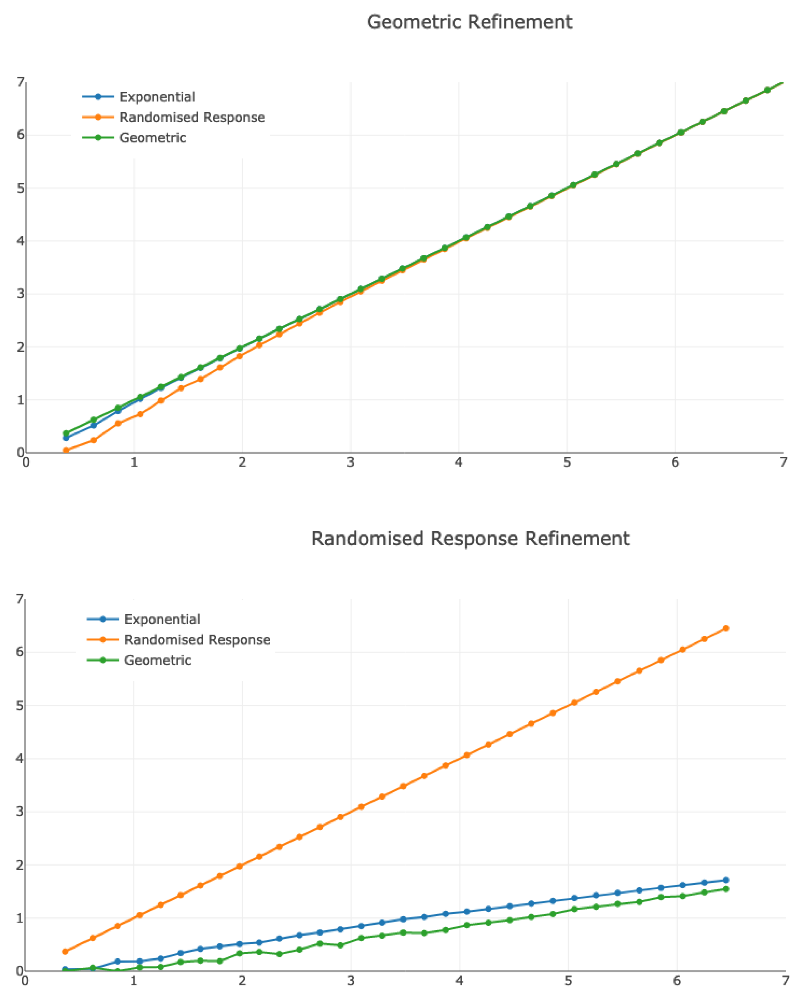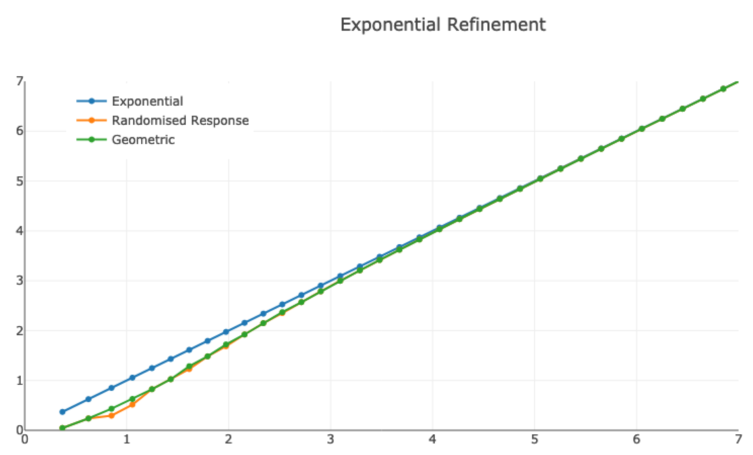For simplicity of presentation, we show results for $5\times 5$ matrices, noting that we observed similar results for experiments across different matrix dimensions, at least wrt the coarse-grained comparison of plots that we do here. The results are plotted in Figure 3.

Figure 3. Refinement of mechanisms under ${⊑}^{\mathrm{avg}}$ for $5\times 5$ channels. The x-axis represents the $\epsilon$ on the LHS of the relation, and the y-axis represents the one on the RHS. The top graph represents refinement of the truncated geometric mechanism (that is, $TG{⊑}^{\mathrm{avg}}$), the middle graph is refinement of randomized response ($R{⊑}^{\mathrm{avg}}$), and the bottom graph is refinement of the exponential mechanism ($E{⊑}^{\mathrm{avg}}$).

The plots show the relationship between ${\epsilon }_1$ (x-axis) and ${\epsilon }_2$ (y-axis) where ${\epsilon }_1$ parametrizes the mechanism being refined and ${\epsilon }_2$ parametrizes the refining mechanism. For example, the blue line on the top graph represents $T{G}^{{\epsilon }_1}{⊑}^{\mathrm{avg}}{E}^{{\epsilon }_2}$. We fix ${\epsilon }_1$ and ask for what value of ${\epsilon }_2$ do we get a ${⊑}^{\mathrm{avg}}$ refinement. Notice that the line ${\epsilon }_1={\epsilon }_2$ corresponds to the same mechanism in both axes (since every mechanism refines itself).

We can see that refining the randomized response mechanism requires much smaller values of epsilon in the other mechanisms. For example, from the middle graph, we can see that $R^4{⊑}^{\mathrm{avg}}T{G}^1$ (approximately) whereas, from the top graph, we have $T{G}^4{⊑}^{\mathrm{avg}}{R}^4$. This means that the randomized response mechanism is very ‘safe’ against average-case adversaries compared with the other mechanisms, as it is much more ‘difficult’ to refine than the other mechanisms.

We also notice that, for ‘large’ values of ${\epsilon }_1$, the exponential and geometric mechanisms refine each other for approximately the same ${\epsilon }_2$ values. This suggests that, for these values, the epsilons are comparable (that is, the mechanisms are equally ‘safe’ for similar values of $\epsilon$). However, smaller values of ${\epsilon }_1$ require a (relatively) large reduction in ${\epsilon }_2$ to obtain a refinement.

6.5. Discussion

At the beginning of this section, we asked whether it is safe to compare differential privacy mechanisms by ‘comparing the epsilons’. We found that it is safe to compare epsilons within families of mechanisms (except in the unusual case of the over-truncated geometric mechanism). However, when comparing different mechanisms, it is not safe to just compare the epsilons, since none of the refinements hold in general. Once a ‘safe’ pair of epsilons has been calculated, then reducing epsilon in the refining mechanism is always safe. However, computing safe epsilons relies on the ability to construct a channel representation, which may not always be feasible.

7. Lattice Properties

The orders ${⊑}^{\mathrm{avg}},{⊑}^{\max }$ and ${⊑}^{\mathrm{prv}}$ are all reflexive and transitive (i.e., preorders), but not anti-symmetric (i.e., not partial orders). This is due to the fact that there exist channels that have “syntactic” differences but the same semantics; e.g., two channels having their columns swapped. However, if we are only interested in a specific type of leakage, then all channels such that $A⊑B⊑A$ (where ⊑ is one of ${⊑}^{\mathrm{avg}},{⊑}^{\max },{⊑}^{\mathrm{prv}}$) have identical leakage, so we can view them as the “same channel” (either by working on the equivalence classes of $⊑\cup ⊒$ or by writing all channels in some canonical form).

Seeing now ⊑ as a partial order, the natural question is whether it forms a lattice that is whether suprema and infima exist. If it exists, the supremum $A\vee B$ has an interesting property: it is the “least safe” channel that is safer than both A and B (any channel C such that $A⊑C$ and $B⊑C$ would necessarily satisfy $A\vee B⊑C$). If we wanted a channel that is safer than both A and B, $A\vee B$ would be a natural choice.

In this section, we briefly discuss this problem and show that—in contrast to ${⊑}^{\mathrm{avg}}$—both ${⊑}^{\max }$ and ${⊑}^{\mathrm{prv}}$ do have suprema and infima (i.e., they form a lattice).

7.1. Average-Case Refinement

In the case of ${⊑}^{\mathrm{avg}}$, “equivalent” channels are those producing the exact same hypers. However, even if we identify such channels, it is known [7] that two channels $A,B$ do not necessarily have a least upper bound wrt ${⊑}^{\mathrm{avg}}$, hence ${⊑}^{\mathrm{avg}}$ does not form a lattice.

7.2. Max-Case Refinement

In the case of ${⊑}^{\max }$, “equivalent” channels are those producing the same posteriors (or more generally the same convex hull of posteriors). However, in contrast to ${⊑}^{\mathrm{avg}}$, if we identify such channels that is if we represent a channel only by the convex hull of its posteriors, then ${⊑}^{\max }$ becomes a lattice.

First, note that given a finite set of posteriors $P=\left\{{\delta }^y\right|y\}$, such that $\pi \in$ch ${\left\{{\delta }^y\right\}}_y$, i.e., such that $\pi ={\sum }_y{a}_y{\delta }^y$, it is easy to construct a channel C producing each posterior ${\delta }^y$ with output probability $a_y$. It suffices to take $C_{x,y}:={\delta }_x^y{a}_y/{\pi }_x$.

Thus, $A{\vee }^{\max }B$ can be simply constructed by taking the intersection of the convex hulls of the posteriors of $A,B$. This intersection is a convex polytope itself, so it has (finitely many) extreme points, so we can construct $A{\vee }^{\max }B$ as the channel having exactly those as posteriors. $A{\wedge }^{\max }B$, on the other hand, can be constructed as the channel having as posteriors the union of those of A and B.

Note that computing the intersection of polytopes is NP-hard in general [21], so $A{\vee }^{\max }B$ might be hard to construct. However, efficient special cases do exist [22]; we leave the study of the hardness of ${\vee }^{\max }$ as future work.

7.3. Privacy-Based Refinement

In the case ${⊑}^{\mathrm{prv}}$, “equivalent” channels are those producing the same induced metric, i.e., ${\mathit{d}}_A={\mathit{d}}_B$. Representing channels only by their induced metric, we can use the fact that $\mathbb{M}\mathcal{X}$ does form a lattice under ≥. We first show that any metric can be turned into a corresponding channel.

Theorem 17.

For any metric $\mathit{d}:\mathbb{M}\mathcal{X}$, we can construct a channel $C^{\mathit{d}}$ such that ${\mathit{d}}_{C^{\mathit{d}}}=\mathit{d}$.

Then, $A{\vee }^{\mathrm{prv}}B$ will be simply the channel whose metric is ${\mathit{d}}_A\vee {\mathit{d}}_B$, where ∨ is the supremum in the lattice of metrics, and similarly for ${\wedge }^{\mathrm{prv}}$.

Note that the infimum of two metrics ${\mathit{d}}_1,{\mathit{d}}_2$ is simply the max of the two (which is always a metric). The supremum, however, is more tricky, since the min of two metrics is not always a metric: the triangle inequality might be violated. Thus, we first need to take the min of ${\mathit{d}}_1,{\mathit{d}}_2$, then compute its “triangle closure”, by finding the shortest path between all pairs of elements, for instance using the well-known Floyd–Warshall algorithm.

8. Conclusions

We have investigated various refinement orders for mechanisms for information protection, combining the max-case perspective typical of DP and its variants with the robustness of the QIF approach. We have provided structural characterizations of these preorders and methods to verify them efficiently. Then, we have considered various DP mechanisms, and investigated the relation between the $\epsilon$-based measurement of privacy and our orders. We have shown that, while within the same family of mechanisms, a smaller $\epsilon$ implies the refinement order, this is almost never the case for mechanisms belonging to different families.