Enhancing Machine Learning Prediction in Cybersecurity Using Dynamic Feature Selector


Abstract
1. Introduction
2. Machine Learning and Cybersecurity
3. Algorithms Used for Dimensionality Reduction
3.1. Univariate Feature Selection
3.2. Correlated Feature Elimination
3.3. Gradient Boosting
3.4. Information Gain
3.5. Wrapper Method Application
4. Dataset Preprocessing
5. Experimental Analysis
5.1. Univariate Feature Selection
5.2. Correlated Feature Elimination
5.3. Gradient Boosting
5.4. Information Gain
5.5. Wrapper Method Application
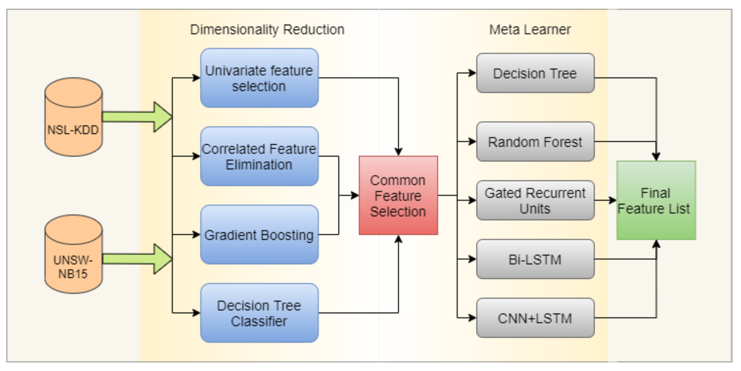
5.6. Dynamic Feature Selection Using a Meta-Learning Approach
| Algorithm 1 Prepare Datasets for Meta-Learners. |
 |
5.7. Meta-Learner
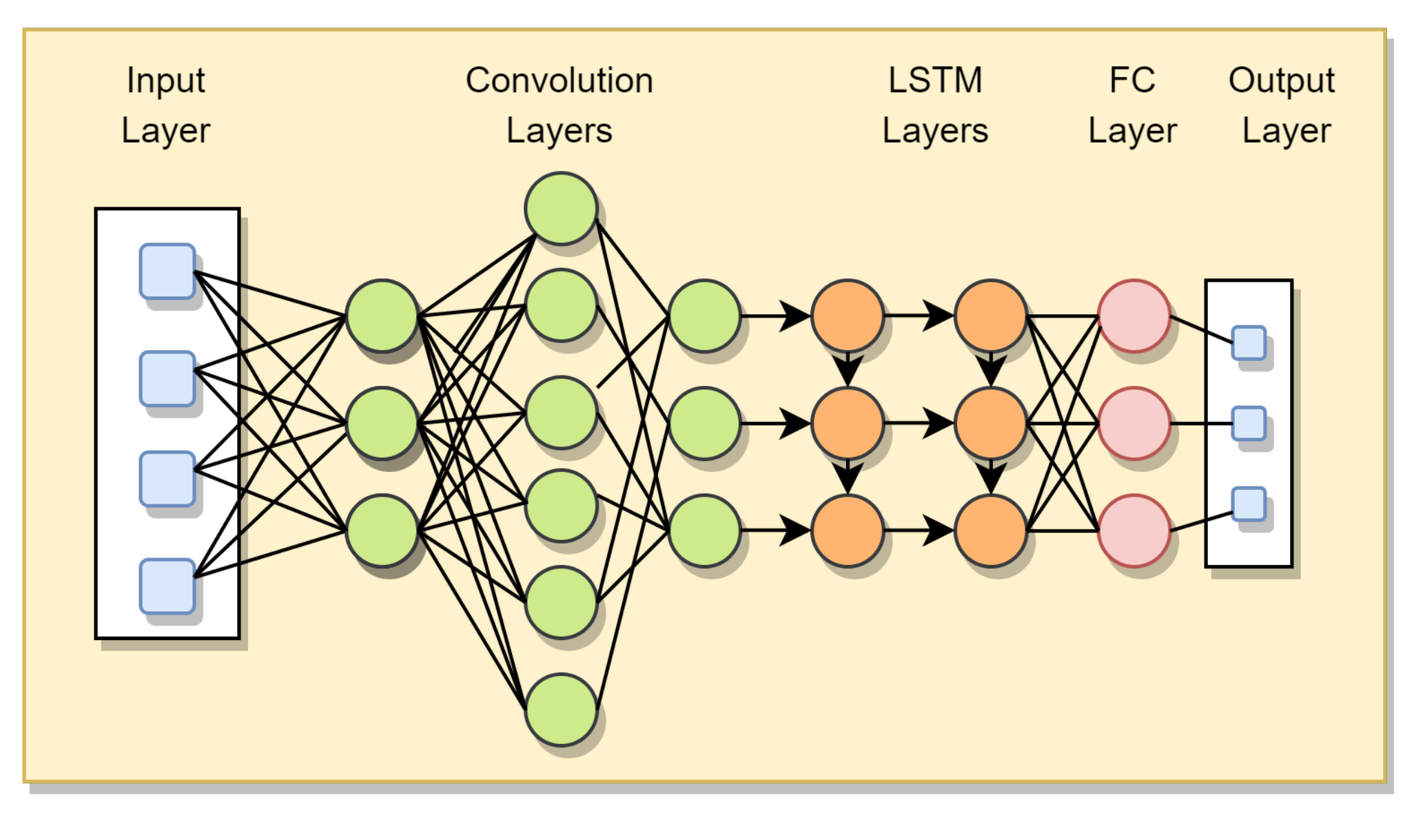
5.7.1. CNN-LSTM
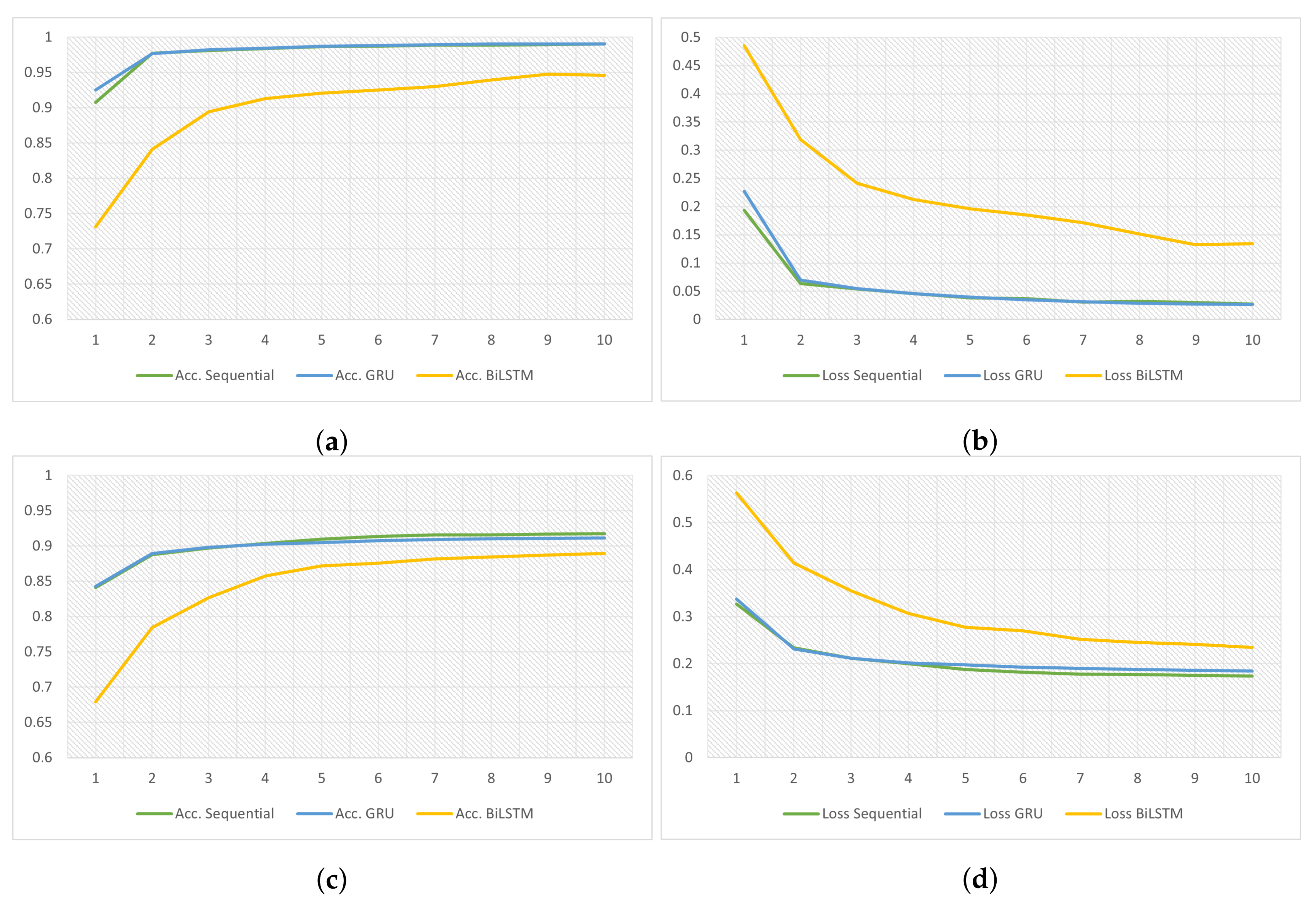
5.7.2. GRU
5.7.3. Bi-LSTM
5.7.4. Decision Trees and Random Forest
5.7.5. Algorithm
| Algorithm 2 Meta-Learners. |
 |
6. Discussion
7. Conclusions
Author Contributions
Funding
Conflicts of Interest
Abbreviations
| RNN | Recurrent Neural Network |
| CNN | Convolutional Nueral Network |
| LSTM | Long Short Term Memory |
| Bi-LSTM | Bidirectional Long Short Term Memory |
| GRU | Gated Recurrent Units |
References
- Chowdhury, M.; Nygard, K. Machine Learning within a Con Resistant Trust Model. In Proceedings of the The 33rd International Conference on Computers and their Applications (CATA 2018), Las Vegas, NV, USA, 19–21 March 2018. [Google Scholar]
- Blum, A.L.; Langley, P. Selection of relevant features and examples in machine learning. Artif. Intell. 1997, 97, 245–271. [Google Scholar] [CrossRef]
- Yang, Y.; Pedersen, J.O. A comparative study on feature selection in text categorization. In Proceedings of the ICML, Nashville, TN, USA, 8–12 July 1997; Volume 97, p. 35. [Google Scholar]
- Breiman, L. Bagging predictors. Mach. Learn. 1996, 24, 123–140. [Google Scholar] [CrossRef]
- Hu, H.; Li, J.; Plank, A.; Wang, H.; Daggard, G. A comparative study of classification methods for microarray data analysis. In Proceedings of the 5th Australasian Data Mining Conference (AusDM 2006): Data Mining and Analytics 2006, Sydney, NSW, Australia, 29–30 November 2006; pp. 33–37. [Google Scholar]
- Niranjan, A.; Prakash, A.; Veena, N.; Geetha, M.; Shenoy, P.D.; Venugopal, K. EBJRV: An Ensemble of Bagging, J48 and Random Committee by Voting for Efficient Classification of Intrusions. In Proceedings of the 2017 IEEE International WIE Conference on Electrical and Computer Engineering (WIECON-ECE), Dehradun, India, 18–19 December 2017; pp. 51–54. [Google Scholar]
- Camargo, C.O.; Faria, E.R.; Zarpelão, B.B.; Miani, R.S. Qualitative evaluation of denial of service datasets. In Proceedings of the XIV Brazilian Symposium on Information Systems, Caxias do Sul, Brazil, 4–8 June 2018; pp. 1–8. [Google Scholar]
- Bachl, M.; Hartl, A.; Fabini, J.; Zseby, T. Walling up Backdoors in Intrusion Detection Systems. In Proceedings of the 3rd ACM CoNEXT Workshop on Big Data, Machine Learning and Artificial Intelligence for Data Communication Networks, Orlando, FL, USA, 9 December 2019; pp. 8–13. [Google Scholar]
- Liu, H.; Liu, Z.; Liu, Y.; Gao, X. Abnormal Network Traffic Detection based on Leaf Node Density Ratio. In Proceedings of the 2019—9th International Conference on Communication and Network Security, Chongqing, China, 15–17 November 2019; pp. 69–74. [Google Scholar]
- Faker, O.; Dogdu, E. Intrusion detection using big data and deep learning techniques. In Proceedings of the 2019 ACM Southeast Conference, Kennesaw, GA, USA, 18–20 April 2019; pp. 86–93. [Google Scholar]
- Thejas, G.; Jimenez, D.; Iyengar, S.S.; Miller, J.; Sunitha, N.; Badrinath, P. COMB: A Hybrid Method for Cross-validated Feature Selection. In Proceedings of the ACM Southeast Regional Conference, Tampa, FL, USA, 2–4 April 2020; pp. 100–106. [Google Scholar]
- Ding, Y.; Zhai, Y. Intrusion detection system for NSL-KDD dataset using convolutional neural networks. In Proceedings of the 2018 2nd International Conference on Computer Science and Artificial Intelligence, Shenzhen, China, 8–10 December 2018; pp. 81–85. [Google Scholar]
- Belouch, M.; Elhadaj, S.; Idhammad, M. A hybrid filter-wrapper feature selection method for DDoS detection in cloud computing. Intell. Data Anal. 2018, 22, 1209–1226. [Google Scholar] [CrossRef]
- Khammassi, C.; Krichen, S. A GA-LR wrapper approach for feature selection in network intrusion detection. Comput. Secur. 2017, 70, 255–277. [Google Scholar] [CrossRef]
- Tun, M.T.; Nyaung, D.E.; Phyu, M.P. Network Anomaly Detection using Threshold-based Sparse. In Proceedings of the 11th International Conference on Advances in Information Technology, Bangkok, Thailand, 1–3 July 2020; pp. 1–8. [Google Scholar]
- Viet, H.N.; Van, Q.N.; Trang, L.L.T.; Nathan, S. Using deep learning model for network scanning detection. In Proceedings of the 4th International Conference on Frontiers of Educational Technologies, Moscow, Russia, 25–27 June 2018; pp. 117–121. [Google Scholar]
- Primartha, R.; Tama, B.A. Anomaly detection using random forest: A performance revisited. In Proceedings of the 2017 International Conference on Data and Software Engineering (ICoDSE), Palembang, Indonesia, 1–2 November 2017; pp. 1–6. [Google Scholar]
- Chen, T.; Guestrin, C. Xgboost: A scalable tree boosting system. In Proceedings of the 22nd acm sigkdd International Conference on Knowledge Discovery and Data Mining, San Francisco, CA, USA, 13–17 August 2016; pp. 785–794. [Google Scholar]
- Belouch, M.; Hadaj, S.E. Comparison of ensemble learning methods applied to network intrusion detection. In Proceedings of the Second International Conference on Internet of things, Data and Cloud Computing, Cambridge, UK, 22–23 March 2017; pp. 1–4. [Google Scholar]
- Liu, J.; Kantarci, B.; Adams, C. Machine learning-driven intrusion detection for Contiki-NG-based IoT networks exposed to NSL-KDD dataset. In Proceedings of the 2nd ACM Workshop on Wireless Security and Machine Learning, Linz, Austria, 13 July 2020; pp. 25–30. [Google Scholar]
- Tran, B.; Xue, B.; Zhang, M. Class dependent multiple feature construction using genetic programming for high-dimensional data. In Australasian Joint Conference on Artificial Intelligence, Proceedings of the AI 2017: AI 2017: Advances in Artificial Intelligence, Melbourne, VIC, Australia, 19–20 August 2017; Springer: Cham, Switzerland, 2017; pp. 182–194. [Google Scholar]
- Krishna, G.J.; Ravi, V. Feature subset selection using adaptive differential evolution: An application to banking. In Proceedings of the ACM India Joint International Conference on Data Science and Management of Data, Kolkata, India, 3–5 January 2019; pp. 157–163. [Google Scholar]
- Wang, L.; Zhou, N.; Chu, F. A general wrapper approach to selection of class-dependent features. IEEE Trans. Neural Netw. 2008, 19, 1267–1278. [Google Scholar] [CrossRef]
- Tran, B.; Zhang, M.; Xue, B. Multiple feature construction in classification on high-dimensional data using GP. In Proceedings of the 2016 IEEE Symposium Series on Computational Intelligence (SSCI), Athens, Greece, 6–9 December 2016; pp. 1–8. [Google Scholar]
- Hariharakrishnan, J.; Mohanavalli, S.; Kumar, K.S. Survey of pre-processing techniques for mining big data. In Proceedings of the 2017 International Conference on Computer, Communication and Signal Processing (ICCCSP), Chennai, India, 10–11 January 2017; pp. 1–5. [Google Scholar]
- Enache, A.C.; Sgarciu, V.; Petrescu-Niţă, A. Intelligent feature selection method rooted in Binary Bat Algorithm for intrusion detection. In Proceedings of the 2015 IEEE 10th Jubilee International Symposium on Applied Computational Intelligence and Informatics, Timisoara, Romania, 21–23 May 2015; pp. 517–521. [Google Scholar]
- Mohammadi, S.; Mirvaziri, H.; Ghazizadeh-Ahsaee, M.; Karimipour, H. Cyber intrusion detection by combined feature selection algorithm. J. Inf. Secur. Appl. 2019, 44, 80–88. [Google Scholar] [CrossRef]
- Goodfellow, I.; Bengio, Y.; Courville, A.; Bengio, Y. Deep Learning; MIT Press: Cambridge, MA, USA, 2016; Volume 1. [Google Scholar]
- Ahsan, M.; Gomes, R.; Denton, A. Application of a Convolutional Neural Network using transfer learning for tuberculosis detection. In Proceedings of the 2019 IEEE International Conference on Electro Information Technology (EIT), Brookings, SD, USA, 20–22 May 2019; pp. 427–433. [Google Scholar]
- Liu, H.; Yu, L. Toward integrating feature selection algorithms for classification and clustering. IEEE Trans. Knowl. Data Eng. 2005, 17, 491–502. [Google Scholar]
- Guyon, I.; Elisseeff, A. An introduction to variable and feature selection. J. Mach. Learn. Res. 2003, 3, 1157–1182. [Google Scholar]
- Kim, T.K. Understanding one-way ANOVA using conceptual figures. Korean J. Anesthesiol. 2017, 70, 22. [Google Scholar] [CrossRef] [PubMed]
- Benesty, J.; Chen, J.; Huang, Y.; Cohen, I. Pearson correlation coefficient. In Noise Reduction in Speech Processing; Springer: Berlin/Heidelberg, Germany, 2009; pp. 1–4. [Google Scholar]
- Benesty, J.; Chen, J.; Huang, Y. On the importance of the Pearson correlation coefficient in noise reduction. IEEE Trans. Audio Speech Lang. Process. 2008, 16, 757–765. [Google Scholar] [CrossRef]
- Friedman, J.H. Greedy function approximation: A gradient boosting machine. Ann. Stat. 2001, 29, 1189–1232. [Google Scholar] [CrossRef]
- Chen, T.; He, T.; Benesty, M.; Khotilovich, V.; Tang, Y. Xgboost: Extreme gradient boosting. R Package Version 0.4-2. 2015, pp. 1–4. Available online: https://mran.microsoft.com/web/packages/xgboost/vignettes/xgboost.pdf (accessed on 15 July 2020).
- Gomes, R.; Denton, A.; Franzen, D. Quantifying Efficiency of Sliding-Window Based Aggregation Technique by Using Predictive Modeling on Landform Attributes Derived from DEM and NDVI. ISPRS Int. J. Geo-Inf. 2019, 8, 196. [Google Scholar] [CrossRef]
- Bennett, K.P. Decision Tree Construction via Linear Programming; Technical Report; University of Wisconsin-Madison Department of Computer Sciences: Madison, WI, USA, 1992. [Google Scholar]
- Harris, E. Information Gain Versus Gain Ratio: A Study of Split Method Biases. In Proceedings of the ISAIM, Fort Lauderdale, FL, USA, 2–4 January 2002. [Google Scholar]
- Hall, M.A.; Smith, L.A. Feature Selection for Machine Learning: Comparing a Correlation-Based Filter Approach to the Wrapper. In Proceedings of the FLAIRS Conference, Orlando, FL, USA, 1–5 May 1999; Volume 1999, pp. 235–239. [Google Scholar]
- Gomes, R.; Ahsan, M.; Denton, A. Random forest classifier in SDN framework for user-based indoor localization. In Proceedings of the 2018 IEEE International Conference on Electro/Information Technology (EIT), Rochester, MI, USA, 3–5 May 2018; pp. 0537–0542. [Google Scholar]
- Pal, M. Random forest classifier for remote sensing classification. Int. J. Remote Sens. 2005, 26, 217–222. [Google Scholar] [CrossRef]
- Mao, K.Z. Orthogonal forward selection and backward elimination algorithms for feature subset selection. IEEE Trans. Syst. Man Cybern. Part B (Cybern.) 2004, 34, 629–634. [Google Scholar] [CrossRef] [PubMed]
- NSL-KDD Dataset. 2020. Available online: https://www.unb.ca/cic/datasets/nsl.html (accessed on 15 July 2020).
- KDD Cup 1999 Data. 2020. Available online: http://kdd.ics.uci.edu/databases/kddcup99/ (accessed on 15 July 2020).
- Tavallaee, M.; Bagheri, E.; Lu, W.; Ghorbani, A.A. A detailed analysis of the KDD CUP 99 data set. In Proceedings of the 2009 IEEE Symposium on Computational Intelligence for Security and Defense Applications, Ottawa, ON, Canada, 8–10 July 2009; pp. 1–6. [Google Scholar]
- Seger, C. An Investigation of Categorical Variable Encoding Techniques in Machine Learning: Binary Versus One-Hot and Feature Hashing. 2018. Available online: https://www.diva-portal.org/smash/record.jsf?pid=diva2%3A1259073&dswid=-2157/ (accessed on 10 November 2020).
- Cerda, P.; Varoquaux, G.; Kégl, B. Similarity encoding for learning with dirty categorical variables. Mach. Learn. 2018, 107, 1477–1494. [Google Scholar] [CrossRef]
- Choong, A.C.H.; Lee, N.K. Evaluation of convolutionary neural networks modeling of DNA sequences using ordinal versus one-hot encoding method. In Proceedings of the 2017 International Conference on Computer and Drone Applications (IConDA), Kuching, Malaysia, 9–11 November 2017; pp. 60–65. [Google Scholar]
- Nguyen, N.G.; Tran, V.A.; Ngo, D.L.; Phan, D.; Lumbanraja, F.R.; Faisal, M.R.; Abapihi, B.; Kubo, M.; Satou, K. DNA sequence classification by convolutional neural network. J. Biomed. Sci. Eng. 2016, 9, 280. [Google Scholar] [CrossRef]
- Cohen, J.; Cohen, P.; West, S.G.; Aiken, L.S. Applied Multiple Regression/Correlation Analysis for the Behavioral Sciences; Lawrence Erlbaum Associates Publishers: Mahwah, NJ, USA, 2013. [Google Scholar]
- Su, T.; Sun, H.; Zhu, J.; Wang, S.; Li, Y. BAT: Deep Learning Methods on Network Intrusion Detection Using NSL-KDD Dataset. IEEE Access 2020, 8, 29575–29585. [Google Scholar] [CrossRef]
- Moustafa, N.; Slay, J. UNSW-NB15: A comprehensive data set for network intrusion detection systems (UNSW-NB15 network data set). In Proceedings of the 2015 military communications and information systems conference (MilCIS), Canberra, ACT, Australia, 10–12 November 2015; pp. 1–6. [Google Scholar]
- Ahsan, M.; Nygard, K.E. Convolutional Neural Networks with LSTM for Intrusion Detection. In Proceedings of the CATA, San Francisco, CA, USA, 23–25 March 2020; pp. 69–79. [Google Scholar]
- Nichol, A.; Achiam, J.; Schulman, J. On first-order meta-learning algorithms. arXiv 2018, arXiv:1803.02999. [Google Scholar]
- Finn, C.; Abbeel, P.; Levine, S. Model-agnostic meta-learning for fast adaptation of deep networks. arXiv 2017, arXiv:1703.03400. [Google Scholar]
- Lemke, C.; Budka, M.; Gabrys, B. Metalearning: A survey of trends and technologies. Artif. Intell. Rev. 2015, 44, 117–130. [Google Scholar] [CrossRef]
- Cruz, R.M.; Sabourin, R.; Cavalcanti, G.D.; Ren, T.I. META-DES: A dynamic ensemble selection framework using meta-learning. Pattern Recognit. 2015, 48, 1925–1935. [Google Scholar] [CrossRef]
- Lin, S.C.; Yuan-chin, I.C.; Yang, W.N. Meta-learning for imbalanced data and classification ensemble in binary classification. Neurocomputing 2009, 73, 484–494. [Google Scholar] [CrossRef]
- Dvornik, N.; Schmid, C.; Mairal, J. Diversity with cooperation: Ensemble methods for few-shot classification. In Proceedings of the IEEE International Conference on Computer Vision, Seoul, Korea, 27 October– 2 November 2019; pp. 3723–3731. [Google Scholar]
- Fu, R.; Zhang, Z.; Li, L. Using LSTM and GRU neural network methods for traffic flow prediction. In Proceedings of the 2016 31st Youth Academic Annual Conference of Chinese Association of Automation (YAC), Wuhan, China, 11–13 November 2016; pp. 324–328. [Google Scholar]
- Dey, R.; Salemt, F.M. Gate-variants of gated recurrent unit (GRU) neural networks. In Proceedings of the 2017 IEEE 60th international midwest symposium on circuits and systems (MWSCAS), Boston, MA, USA, 6–9 August 2017; pp. 1597–1600. [Google Scholar]
- Chang, L.Y.; Chen, W.C. Data mining of tree-based models to analyze freeway accident frequency. J. Saf. Res. 2005, 36, 365–375. [Google Scholar] [CrossRef] [PubMed]
- Aldous, D. Tree-based models for random distribution of mass. J. Stat. Phys. 1993, 73, 625–641. [Google Scholar] [CrossRef]
- Yang, Y.; Morillo, I.G.; Hospedales, T.M. Deep neural decision trees. arXiv 2018, arXiv:1806.06988. [Google Scholar]
- Zhang, J.; Man, K. Time series prediction using RNN in multi-dimension embedding phase space. In Proceedings of the 1998 IEEE International Conference on Systems, Man, and Cybernetics (Cat. No. 98CH36218), San Diego, CA, USA, 14 October 1998; Volume 2, pp. 1868–1873. [Google Scholar]
- Zhang, L.; Xiang, F. Relation classification via BiLSTM-CNN. In International Conference on Data Mining and Big Data, Proceedings of the DMBD 2018: Data Mining and Big Data, Shanghai, China, 17–22 June 2018; Springer: Cham, Switzerland, 2018; pp. 373–382. [Google Scholar]
- Sharfuddin, A.A.; Tihami, M.N.; Islam, M.S. A deep recurrent neural network with bilstm model for sentiment classification. In Proceedings of the 2018 International Conference on Bangla Speech and Language Processing (ICBSLP), Sylhet, Bangladesh, 21–22 September 2018; pp. 1–4. [Google Scholar]
- Powers, D.M. Evaluation: From precision, recall and F-measure to ROC, informedness, markedness and correlation. arXiv 2011, arXiv:2010.16061. [Google Scholar]


| UNSW NB-15 Features | NSL KDD Features | ||
|---|---|---|---|
| rate | sttl | count | logged_in |
| dload | swin | srv_serror_rate | serror_rate |
| stcpb | dtcpb | dst_host_srv_count | same_srv_rate |
| dwin | dmean | dst_host_serror_rate | dst_host_same_srv_rate |
| ct_srv_src | ct_state_ttl | service_http | dst_host_srv_serror_rate |
| ct_src_dport_ltm | ct_dst_sport_ltm | flag_S0 | service_private |
| ct_dst_src_ltm | ct_src_ltm | flag_SF | |
| ct_srv_dst | proto_tcp | ||
| service_dns | state_CON | ||
| state_FIN | state_INT | ||
| UNSW NB-15 Dataset | NSL-KDD Dataset | ||||
|---|---|---|---|---|---|
| Feature | Corr. Feature | Corr. | Feature | Corr. Feature | Corr. |
| sbytes | spkts | 0.964 | num_root | num_compromised | 0.998 |
| dbytes | dpkts | 0.973 | is_guest_login | hot | 0.860 |
| sloss | spkts | 0.972 | srv_serror_rate | serror_rate | 0.993 |
| sloss | sbytes | 0.996 | srv_rerror_rate | rerror_rate | 0.989 |
| dloss | dpkts | 0.979 | dst_host_same_srv_rate | dst_host_srv_count | 0.897 |
| dloss | dbytes | 0.997 | dst_host_serror_rate | serror_rate | 0.979 |
| dwin | swin | 0.981 | dst_host_serror_rate | srv_serror_rate | 0.978 |
| synack | tcprtt | 0.946 | dst_host_srv_serror_rate | serror_rate | 0.981 |
| ackdat | tcprtt | 0.919 | dst_host_srv_serror_rate | srv_serror_rate | 0.986 |
| ct_dst_ltm | ct_srv_src | 0.841 | dst_host_srv_serror_rate | dst_host_serror_rate | 0.985 |
| ct_src_dport_ltm | ct_srv_src | 0.862 | dst_host_rerror_rate | rerror_rate | 0.927 |
| ct_src_dport_ltm | ct_dst_ltm | 0.961 | dst_host_rerror_rate | srv_rerror_rate | 0.918 |
| ct_dst_sport_ltm | ct_srv_src | 0.815 | dst_host_srv_rerror_rate | rerror_rate | 0.964 |
| ct_dst_sport_ltm | ct_dst_ltm | 0.871 | dst_host_srv_rerror_rate | srv_rerror_rate | 0.970 |
| ct_dst_sport_ltm | ct_src_dport_ltm | 0.908 | dst_host_srv_rerror_rate | dst_host_rerror_rate | 0.925 |
| ct_dst_src_ltm | ct_srv_src | 0.954 | service_ftp | is_guest_login | 0.820 |
| ct_dst_src_ltm | ct_dst_ltm | 0.857 | flag_REJ | rerror_rate | 0.835 |
| ct_dst_src_ltm | ct_src_dport_ltm | 0.872 | flag_REJ | srv_rerror_rate | 0.841 |
| ct_dst_src_ltm | ct_dst_sport_ltm | 0.836 | flag_REJ | dst_host_rerror_rate | 0.813 |
| ct_ftp_cmd | is_ftp_login | 0.999 | flag_REJ | dst_host_srv_rerror_rate | 0.829 |
| ct_src_ltm | ct_dst_ltm | 0.901 | |||
| NSL KDD Features | UNSW NB-15 Features | ||
|---|---|---|---|
| duration | src_bytes | dpkts | dur |
| wrong_fragment | num_failed_logins | rate | sbytes |
| logged_in | root_shell | dload | dttl |
| count | dst_host_count | swin | sloss |
| dst_host_srv_count | dst_host_same_srv_rate | ackdat | tcprtt |
| dst_host_diff_srv_rate | dst_host_same_src_port_rate | response_body_len | trans_depth |
| dst_host_srv_diff_host_rate | dst_host_serror_rate | ct_state_ttl | ct_srv_src |
| dst_host_rerror_rate | diffic | ct_src_dport_ltm | ct_dst_ltm |
| Protocol_type_icmp | Protocol_type_tcp | ct_ftp_cmd | ct_dst_sport_ltm |
| service_IRC | service_echo | ct_src_ltm | ct_flw_http_mthd |
| service_eco_i | service_efs | proto_any | proto_3pc |
| service_exec | service_ftp | proto_ax.25 | proto_aris |
| service_ftp_data | service_gopher | proto_ddp | proto_br-sat-mon |
| service_http | service_http_2784 | proto_i-nlsp | proto_fc |
| service_http_8001 | service_ldap | proto_idrp | proto_idpr |
| service_login | service_netbios_ns | proto_igp | proto_ifmp |
| service_nnsp | service_ntp_u | proto_ipv6-frag | proto_ipcv |
| service_pm_dump | service_red_i | proto_netblt | proto_iso-tp4 |
| service_remote_job | service_supdup | proto_pvp | proto_pgm |
| service_telnet | service_tftp_u | proto_sdrp | proto_scps |
| service_uucp | service_uucp_path | proto_tlsp | proto_secure-vmtp |
| service_vmnet | service_whois | proto_trunk-2 | proto_tp++ |
| flag_REJ | flag_RSTO | proto_vines | proto_ttp |
| flag_RSTR | flag_S1 | proto_wb-mon | |
| flag_S3 | flag_SF | ||
| Features | XGBoost Imp. | Inf. Gain | Features | XGBoost Imp. | Inf. Gain |
|---|---|---|---|---|---|
| dst_host_srv_count | 383.4 | 0.4179 | count | 275.3 | 0.4164 |
| diffic | 1223.5 | 0.2612 | dst_host_count | 309.4 | 0.2089 |
| dst_host_diff_srv_rate | 306.4 | 0.4518 | dst_host_rerror_rate | 269 | 0.0979 |
| dst_host_same_src_port_rate | 206.1 | 0.2358 | dst_host_same_srv_rate | 336.4 | 0.4004 |
| dst_host_serror_rate | 273.2 | 0.3986 | dst_host_srv_diff_host_rate | 309 | 0.2614 |
| duration | 196.3 | 0.0647 | flag_SF | 58.4 | 0.4892 |
| logged_in | 123.9 | 0.3063 | root_shell | 176.5 | 0.0018 |
| service_http | 98.4 | 0.0011 | src_bytes | 1321.7 | 0.7202 |
| Features | XGBoost Imp. | Inf. Gain | Features | XGBoost Imp. | Inf. Gain |
|---|---|---|---|---|---|
| sbytes | 2423.9 | 0.4722 | dtcpb | 1575.6 | 0.3811 |
| ct_srv_src | 1572.6 | 0.0827 | stcpb | 1519.7 | 0.3813 |
| ackdat | 1311.9 | 0.3401 | ct_srv_dst | 1215.6 | 0.0974 |
| tcprtt | 1098.5 | 0.3599 | dur | 1033.7 | 0.5392 |
| ct_src_ltm | 911 | 0.0745 | dload | 891.1 | 0.4938 |
| ct_dst_ltm | 712.2 | 0.0833 | rate | 664.1 | 0.5397 |
| dmean | 663.9 | 0.2837 | response_body_len | 506.2 | 0.0359 |
| ct_src_dport_ltm | 462.9 | 0.0941 | ct_dst_sport_ltm | 379.1 | 0.1502 |
| sloss | 321.8 | 0.1098 | ct_state_ttl | 281.1 | 0.3137 |
| dwin | 231.4 | 0.0582 | dpkts | 177.1 | 0.2427 |
| ct_flw_http_mthd | 152.8 | 0.0009 | is_ftp_login | 115.6 | 0.0001 |
| service_dns | 102.3 | 0.0368 | trans_depth | 92.3 | 0.0001 |
| service_http | 91.9 | 0.00006 | proto_tcp | 79.5 | 0.0677 |
| state_CON | 49 | 0.0616 | state_FIN | 25.4 | 0.0479 |
| state_INT | 22.2 | 0.1473 |
| NSL- KDD | Performance without Dynamic Feature Selector | Performance with Dynamic Feature Selector | ||||||||
|---|---|---|---|---|---|---|---|---|---|---|
| CNN+ LSTM | GRU | Bi- LSTM | Decision Trees | Random Forest | CNN+ LSTM | GRU | Bi- LSTM | Decision Trees | Random Forest | |
| Accuracy | 98.96 | 97.04 | 95.47 | 97.94 | 99.37 | 99.1 | 99.04 | 95.15 | 99.63 | 99.65 |
| F1 | 98.21 | 98.43 | 93.50 | 98.01 | 99.33 | 99.15 | 99 | 95.05 | 99.62 | 99.63 |
| Precision | 96.92 | 97.74 | 95.70 | 98.79 | 99.63 | 99.35 | 98.74 | 96.6 | 99.78 | 99.84 |
| AUC | 98.93 | 98.72 | 96.45 | 97.13 | 99.54 | 99.17 | 99.05 | 95.15 | 99.63 | 99.64 |
| UNSW- NB15 | Performance without Dynamic Feature Selector | Performance with Dynamic Feature Selector | ||||||||
|---|---|---|---|---|---|---|---|---|---|---|
| CNN+ LSTM | GRU | Bi- LSTM | Decision Trees | Random Forest | CNN+ LSTM | GRU | Bi- LSTM | Decision Trees | Random Forest | |
| Accuracy | 91 | 90.12 | 88.93 | 85.31 | 90.98 | 91.91 | 90.75 | 89.28 | 86.8 | 92.76 |
| F1 | 92.07 | 91.24 | 90.32 | 88.96 | 93.35 | 93.7 | 93.08 | 91.53 | 89.5 | 94.44 |
| Precision | 91.4 | 97.84 | 91.89 | 87.99 | 95.96 | 94.23 | 97.35 | 90.61 | 88.01 | 96.11 |
| AUC | 91 | 90.87 | 88.43 | 84.91 | 91.74 | 91.38 | 91.78 | 88.2 | 85.49 | 92.73 |
Publisher’s Note: MDPI stays neutral with regard to jurisdictional claims in published maps and institutional affiliations. |
© 2021 by the authors. Licensee MDPI, Basel, Switzerland. This article is an open access article distributed under the terms and conditions of the Creative Commons Attribution (CC BY) license (http://creativecommons.org/licenses/by/4.0/).
Share and Cite
Ahsan, M.; Gomes, R.; Chowdhury, M.M.; Nygard, K.E. Enhancing Machine Learning Prediction in Cybersecurity Using Dynamic Feature Selector. J. Cybersecur. Priv. 2021, 1, 199-218. https://doi.org/10.3390/jcp1010011
Ahsan M, Gomes R, Chowdhury MM, Nygard KE. Enhancing Machine Learning Prediction in Cybersecurity Using Dynamic Feature Selector. Journal of Cybersecurity and Privacy. 2021; 1(1):199-218. https://doi.org/10.3390/jcp1010011
Chicago/Turabian StyleAhsan, Mostofa, Rahul Gomes, Md. Minhaz Chowdhury, and Kendall E. Nygard. 2021. "Enhancing Machine Learning Prediction in Cybersecurity Using Dynamic Feature Selector" Journal of Cybersecurity and Privacy 1, no. 1: 199-218. https://doi.org/10.3390/jcp1010011
APA StyleAhsan, M., Gomes, R., Chowdhury, M. M., & Nygard, K. E. (2021). Enhancing Machine Learning Prediction in Cybersecurity Using Dynamic Feature Selector. Journal of Cybersecurity and Privacy, 1(1), 199-218. https://doi.org/10.3390/jcp1010011