A Comprehensive Evaluation of Earthquake Losses in Indonesia: A Multi-Indicator Index Based on Grey Relational Analysis

Abstract

Indonesia experiences some of the world’s highest seismic activity, making earthquakes a major source of physical, economic, and social losses. To better quantify these impacts, this study proposes a comprehensive evaluation framework with two new metrics: the Seismic Severity Index (SSI) and the Seismic Impact Index (SII). The indices are derived using four weighting methods—Grey Relational Analysis (GRA), Equal Weights, the Entropy Weight Method (EWM), and Criteria Importance Through Intercriteria Correlation (CRITIC)—and applied to 28 regencies and municipalities affected by damaging earthquakes from 2016 to 2022. Results show that the 2018 earthquake, intensified by a tsunami and liquefaction, caused the most severe losses. Palu Municipality and Donggala Regency consistently recorded high SSI values across all weighting schemes. The SII further identifies Sigi Regency, Donggala Regency, and Palu Municipality as the most heavily impacted areas, although rankings varied by method. Overall, Sigi Regency, Palu City, Donggala Regency, North Lombok, West Lombok and Cianjur exhibit the highest combined severity and impact, while Garut, Ciamis, and Cilacap experienced relatively minor effects. The study concludes that integrating GRA with EWM and CRITIC yields a robust earthquake loss index to support future disaster risk reduction policies.

1. Introduction

Earthquakes are devastating natural disasters that cause significant economic losses, physical damage, casualties, and regional economic disruption [1,2,3,4]. Between 2004 and 2023, EM-DAT data show that earthquakes were responsible for 56.24% of all natural disaster-related deaths, resulting annually in an average of 36.88 million fatalities, 6.8 million people affected, and US$43.5 billion in economic losses [5]. Increased earthquake losses are determined not only by ground shaking intensity and the level of building structure exposure. However, they are also significantly influenced by geotechnical hazards such as liquefaction, lateral spreading, and soil amplification [6,7]. These processes can cause severe soil deformation, resulting in significant damage to buildings, vital infrastructure networks, and underground infrastructure systems, while also hindering post-disaster recovery efforts [6]. Given these profound impacts, accurate earthquake disaster loss measurement is fundamental for effective disaster risk management, guiding mitigation priorities, resource allocation, and recovery strategies [8,9].

The Sendai Framework for Disaster Risk Reduction (SFDRR) 2015–2030 underscores the importance of collecting comprehensive and comparable loss data to improve accountability and efficacy of DRR policies [10,11]. It includes four key targets (A, B, C, D) that mandate the reporting of disaster loss data, covering fatalities, affected populations, economic losses relative to GDP, and damage to critical infrastructure, particularly health and education facilities [11]. While estimating both direct and indirect economic losses is crucial for understanding vulnerabilities and designing sustainable reconstruction efforts [12], current loss measurement often falls short by focusing solely on direct economic losses or physical damage, thus failing to capture the full complexity of earthquake impacts on regional systems.

Indonesia’s location on the Pacific Ring of Fire, where the Eurasian, Indo-Australian, and Pacific tectonic plates converge, makes it exceptionally vulnerable to earthquakes [13,14,15]. The subduction processes between these plates not only triggers high seismic activity but also form a chain of active volcanoes scattered throughout Indonesia. The presence of 129 active volcanoes further contributes to its high seismic and volcanic activity, making it one of the world’s most earthquake-prone nations [14,16].

High volcanic activity can trigger various secondary disasters, such as volcanic earthquakes, pyroclastic flows, volcanic landslides, and tsunamis. One example is the 2018 Anak Krakatau event, when the partial collapse of the volcano and the resulting debris flow triggered a tsunami in the Sunda Strait, causing widespread damage and loss of life along the coasts of Banten and Lampung, despite the absence of a major tectonic earthquake [17]. This event demonstrates that tectonic and volcanic dynamics in Indonesia are interrelated and collectively contribute to the high risk of geological disasters in this region.

Previous research has explored composite index-based methods for disaster loss assessment [18,19,20,21]. For instance, Zhao et al. (2024) developed Disaster Severity and Impact Indices for Shanghai using AHP and EWM [21]. However, these studies often lack direct comparisons with nonparametric methods like grey Relational Analysis (GRA) and rarely develop earthquake-specific loss indices. This highlights a gap in understanding how methodological choices influence loss measurement and the ranking of affected areas, particularly as most prior disaster loss indices were developed at the national level with limited comparative analyses.

Significant gaps persist in the literature. Firstly, there is a lack of integration between objective weighting methods like Entropy and CRITIC, which could provide more stable and representative weights. Secondly, the application of grey Relational Analysis (GRA) to earthquake losses, especially in developing countries such as Indonesia, remains rare despite its suitability for systems with limited data and high uncertainty. Thirdly, Indonesian research often prioritizes risk and exposure analysis over comprehensive, multi-indicator loss measurement. Previous studies suggest that GRA can enhance the accuracy of identifying key factors in earthquake losses [22]. Thus, a more integrated and context-specific approach is urgently needed.

To address these limitations, this study distinguishes between measures of the absolute and relative impacts of earthquakes. Previous approaches to disaster loss assessment have generally relied on absolute indicators such as the number of fatalities or total economic losses. However, such measures tend to be biased toward regions with large populations or high economic capacity. Therefore, this study integrates normalized indicators, such as impact per capita and economic losses relative to Regional Gross Domestic Product (RGDP), to represent the burden of disasters more proportionally.

Based on this approach, this study proposes two indices: the Seismic Severity Index (SSI) and the Seismic Impact Index (SII). SSI represents the total human, physical, and economic losses in absolute terms. At the same time, SII describes the relative impact by considering the region’s population size and economic capacity. This index framework enables more relevant analysis for decision-making, particularly in identifying regions that bear a disproportionate disaster burden.

Therefore, this study aims to address these gaps by developing an Earthquake Loss Index, comprising the Seismic Severity Index (SSI) and the Seismic Impact Index (SII), at the district/city level. This is achieved by integrating grey Relational Analysis (GRA) with the Entropy–CRITIC objective weighting method to create a comprehensive and robust measure of earthquake-induced losses. Methodologically, this research will illuminate the strengths and limitations of GRA compared to conventional composite index approaches in disaster loss assessment. Empirically, it will offer a more sensitive, spatially explicit mapping of earthquake losses by capturing regional heterogeneity, thereby informing more targeted, evidence-based policies for disaster risk reduction, mitigation, recovery, and post-disaster reconstruction. The development of this Earthquake Loss Index and the innovative integration of GRA with Entropy-CRITIC promise to significantly advance loss assessment practices for researchers and practitioners alike.

This article is structured into several sections: an introduction outlining the background, problems, and objectives; a literature review on disaster loss measurement and GRA; a methodology section detailing indicator construction and the integration of Entropy, CRITIC, and GRA, along with scope and limitations; an empirical analysis of earthquake loss levels in Indonesia, including a discussion of spatial patterns and influencing factors; and finally, a conclusion summarizing findings and offering strategic recommendations for earthquake risk reduction in Indonesia.

2. Literature Review

Earthquake disasters are one of the largest sources of losses in disaster risk studies due to their sudden nature and potential impact on socioeconomic systems. Various approaches have been developed to assess earthquake losses, including earthquake disaster loss assessments [3,23], impact modeling [24,25], and seismic risk analysis [26], all of which contribute to a better understanding of potential impacts. These approaches focus on absolute indicators such as fatalities, physical damage, and economic losses [3,23]. However, the use of absolute indicators alone is often insufficient to represent the relative pressure on a region’s capacity, particularly socioeconomic disparities between regions.

In response to these limitations, composite index-based approaches have emerged to integrate various dimensions of loss more systematically. Multi-indicator indices allow for the combination of human, physical, and economic dimensions into a single measure, thereby enhancing comparability across regions and the ability to capture variations in impacts that are not apparent in single indicators. Previous studies, such as Zhao et al. [21], emphasize the importance of distinguishing between severity (the level of hazard severity) and impact (the realization of the impact), given that losses are determined not only by hazard intensity but also by regional exposure and mitigation capacity.

Recent literature also indicates that seismic hazards do not influence disaster losses not only directly, but also through geotechnical and multi-hazard processes. Indonesia’s location on the Pacific Ring of Fire means that high seismic activity goes hand in hand with high volcanic activity [17]. Processes such as liquefaction, landslides, ground deformation, and volcanic collapse can significantly amplify the impact of losses. The 2018 event at Anak Krakatau demonstrated that a tsunami can be triggered by volcanic collapse without being preceded by a major earthquake, with a collapse volume of approximately 0.2–0.3 km³ capable of reproducing the observed tsunami characteristics. This finding confirms that non-seismic mechanisms also contribute to loss indicators such as fatalities, displacement, and economic losses.

From a methodological perspective, various multi-criteria decision analysis (MCDA) approaches have been used to measure disaster losses, including AHP, TOPSIS, PROMETHEE, GRA, and composite indices [18,21,27,28]. Among these methods, Grey Relational Analysis (GRA) is employed due to its ability to analyze systems with limited, heterogeneous data and nonlinear relationships. Based on grey system theory, GRA does not require specific distribution assumptions and allows for the evaluation of relational proximity between indicators through the concept of relational grade [2,29,30,31]. Therefore, this method is considered relevant for the context of disaster data, which is often incomplete and has a high degree of uncertainty.

Nevertheless, research on disaster loss indices remains dominated by studies of regions or countries with relatively good data availability, while its application in developing countries with high geographical complexity, such as Indonesia, remains limited. Furthermore, the conceptual distinction between hazard severity and loss impacts at the subnational level has not been extensively explored in the existing literature.

3. Materials and Methods

In this study, we introduce a comprehensive framework for earthquake loss assessment that enables comparison of losses across districts and cities. The approach focuses on evaluating how earthquake losses are distributed among administrative regions to reveal patterns of inequality in disaster impacts. It combines the Seismic Severity Index (SSI), which measures absolute losses, with the Seismic Impact Index (SII), which captures the relative impact on regional capacity. Together, these indices provide a deeper understanding of spatial variations in earthquake severity and consequences, as illustrated in Figure 1.

3.1. Data

The unit of analysis in this study is districts and cities that experienced damaging earthquakes between 2016 and 2022. This period was selected based on data completeness and consistency in reporting damage and loss values resulting from disasters, as documented in the Post-Disaster Rehabilitation and Reconstruction Plans (RRRP) submitted by local governments at the district/city levels and published by the National Disaster Management Agency (BNPB). Earlier events were excluded due to incomplete variable availability, while more recent events fell outside the final dataset used in this analysis. Based on these criteria, 28 districts and municipalities across 15 provinces were selected. The data in this study consists of event-based cross-sectional data, where each observation represents the impact of an earthquake on a specific region during a particular event, and thus does not form panel data or a time series. Furthermore, for regions that experienced multiple destructive earthquakes during the 2016–2022 period, such as the 2018 Lombok Earthquake and the 2028 Palu Earthquake, disaster losses were aggregated using a cumulative event-based approach based on official BNPB reports.

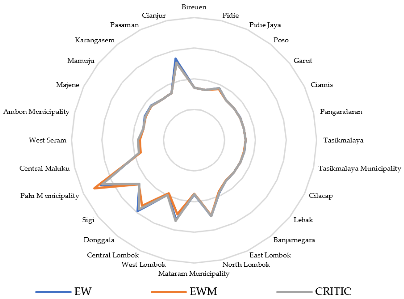
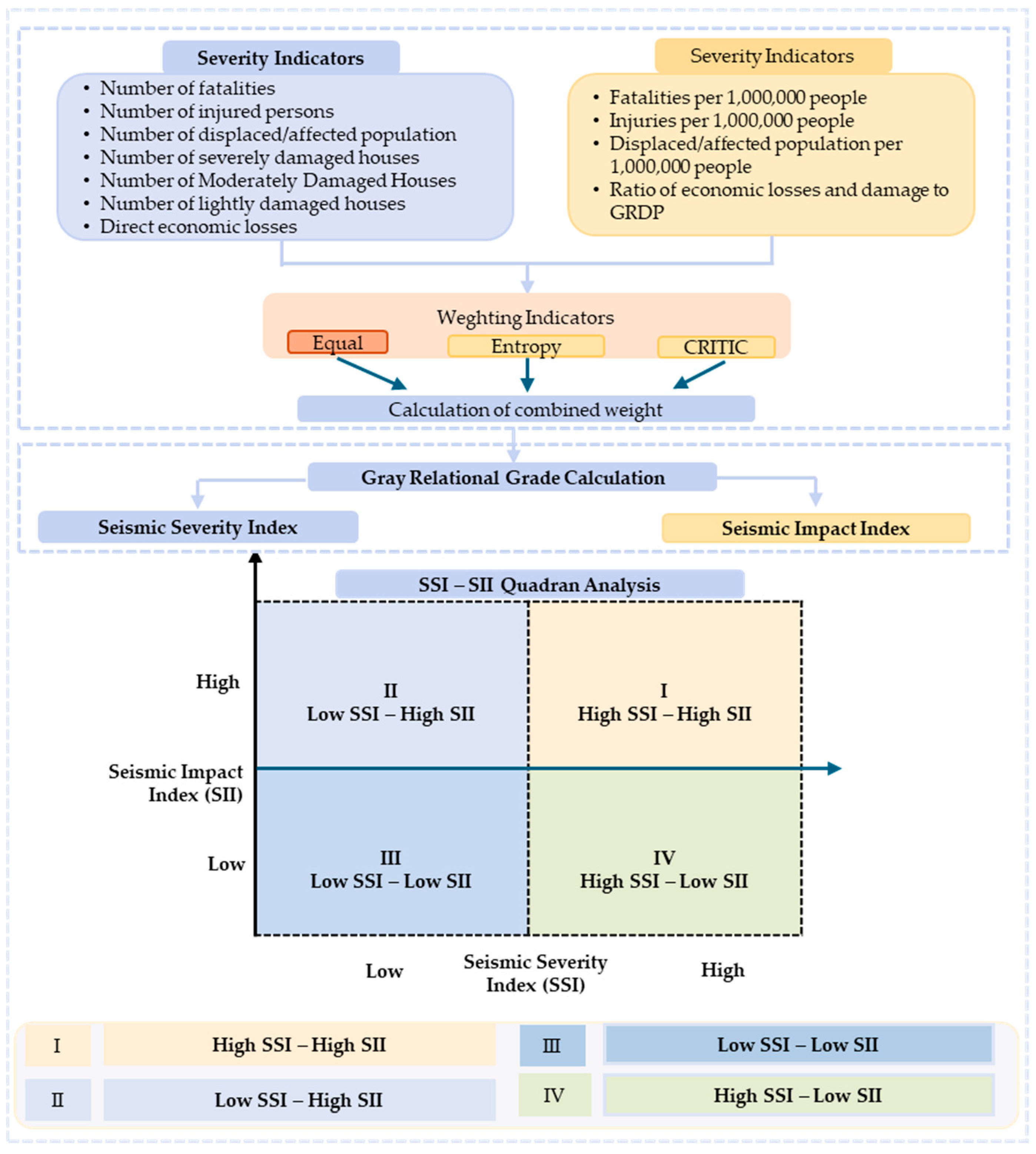
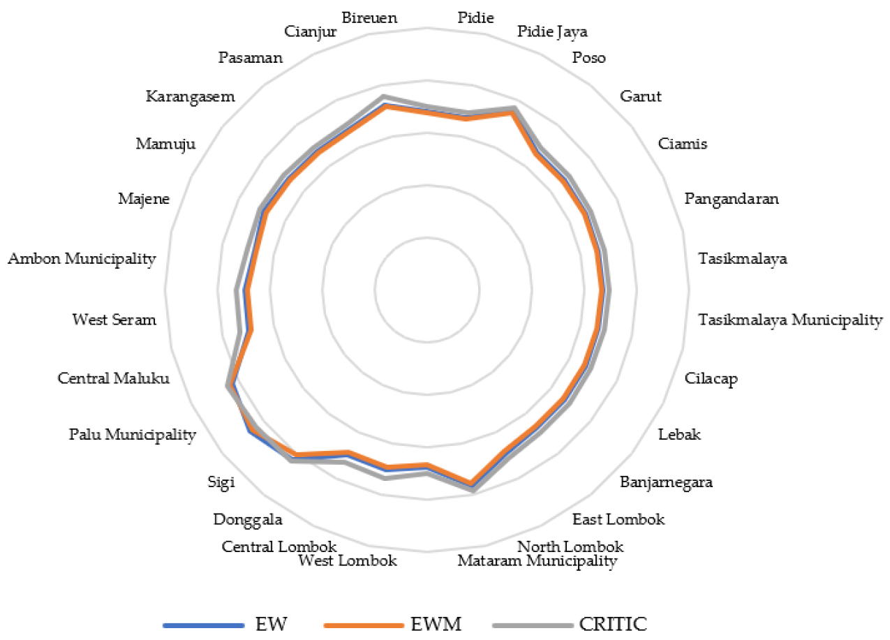
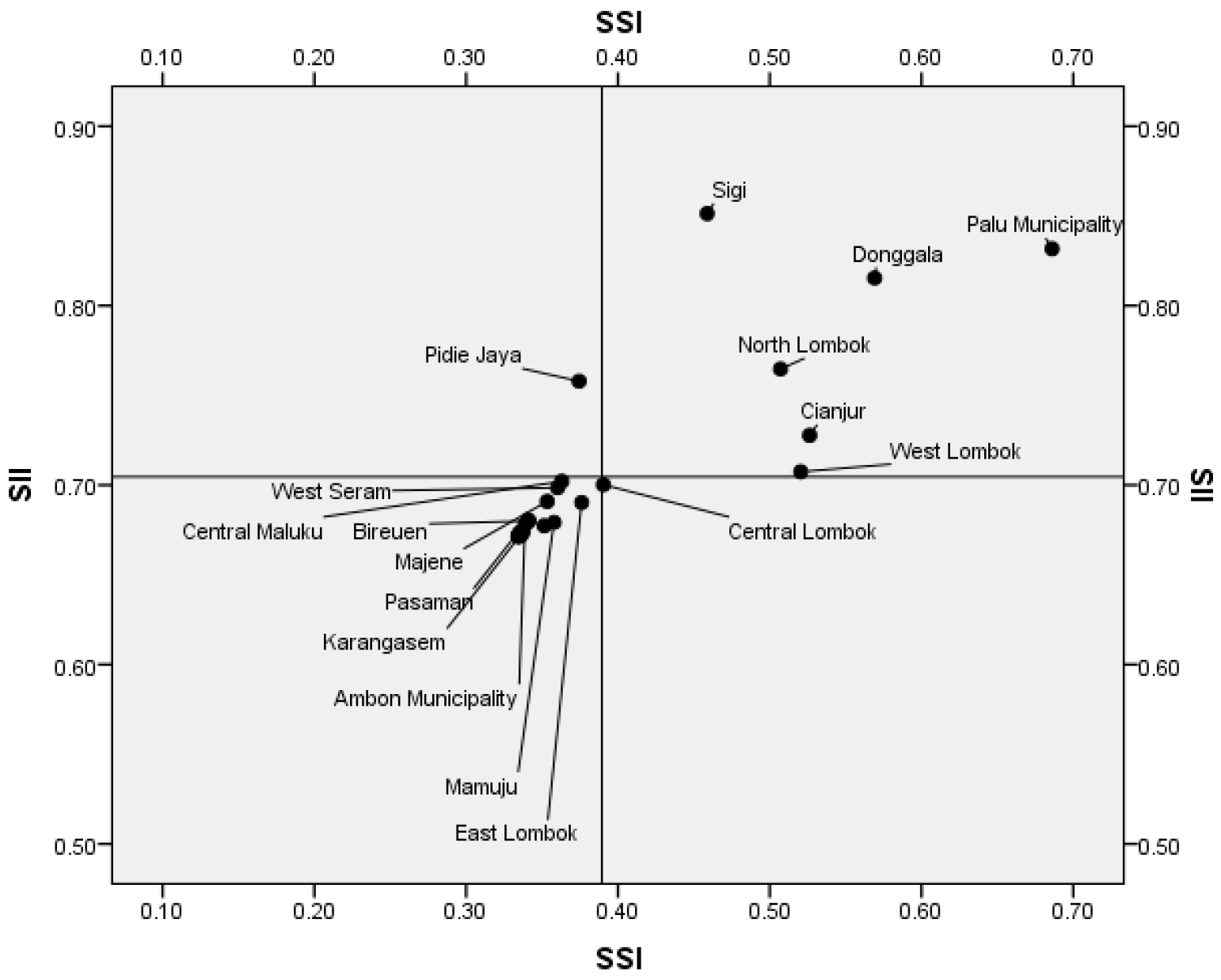
The earthquake loss index comprises two components: the Seismic Severity Index (SSI) and the Seismic Impact Index (SII), which together characterize earthquake-related losses. The SSI captures the absolute losses caused by an earthquake, whereas the SII measures losses relative to local capacity and exposure, normalized by population and economic size. Accordingly, the SSI represents the absolute intensity and outcomes of the earthquake, while the SII indicates the level of stress and relative vulnerability of the affected area. Integrating both indices offers a more holistic and quantifiable basis for evaluating earthquake losses.

The construction of the earthquake severity and impact indices follows an approach consistent with Zhao et al. [21] and draws on key indicators developed by Zhao et al. [21], Li et al. [18], Miao et al. [32], and Haoying et al. [2]. The indicators used in this study focus on the direct impacts of disasters, including deaths, injuries, affected populations, housing damage, and direct economic losses. This study did not explicitly include indirect losses and infrastructure disruptions due to limitations in data availability and consistency across the study areas. Nevertheless, researchers widely use these direct loss indicators in the disaster literature as key proxies for assessing earthquake impacts.

Indicators were selected for their relevance to earthquake impact assessment, availability at the district/city level, and demonstrated effectiveness in previous research. The selection process involved two stages. First, a literature review was conducted on the measurement of earthquake severity and impact indices, including the studies by Zhao et al. [21], Li et al. [18], Miao et al. [32], and Haoying et al. [2]. Second, the indicators were adapted to the Indonesian context and to the availability of subnational data in publications from the Central Statistics Agency (BPS) and the National Agency for Disaster Countermeasure (BNPB). In total, 7 indicators were used to calculate the SSI and 4 indicators to construct the SII, along with their directions of influence, as presented in

Table 1. Seismic Loss Index Indicators.

Indicators	Unit	Ref.	Data Sources	Reference
Seismic Severity Index (SSI)
Number of fatalities	person	+	BNPB	[2,18,21,32]
Number of injured persons	person	+	BNPB	[2,11,18,21]
Number of displaced/affected people	person	+	BNPB	[11,18,21,32]
Number of Severely Damaged Houses	Unit	+	BNPB	[2,11,18,21]
Number of Moderately Damaged Houses	Unit	+	BNPB	[2,11,18,21]
Number of Lightly Damaged Houses	Unit	+	BNPB	[2,11,18,21]
Direct economic loss	Rupiah	+	BNPB	[2,11,18,21,32]
Seismic Impact Index (SII)
Fatalities	Deaths per million population	+	BNPB, BPS	[18,21]
Injuries	Injuries per million population	+	BNPB, BPS	[18]
Affected population	Affected persons per million population	+	BNPB, BPS	[18,21]
Ratio of economic losses and damage to GRDP	-	+	BNPB, BPS	[18,21]

Note: “+” is for benefit indicators, and “-” is for cost indicators.

.

3.2. Analysis Method

This study employs a Multi-Criteria Decision-Making (MCDM) approach based on grey system theory, originally proposed by Deng Julong in 1982 [33]. This approach is designed to evaluate relationships among factors in systems characterized by limited or incomplete information [2]. The analysis integrates Grey Relational Analysis (GRA) with the Entropy–CRITIC weighting technique. GRA is used to measure and compare earthquake losses across Indonesian districts/cities affected by earthquakes during 2016–2022 and to identify key factors influencing the Seismic Loss Index (SLI) based on geometric correspondence among indicators. A grey relational grade (GRG) for an SLI indicator greater than 0.5 denotes a close correlation, while a GRG exceeding 0.7 indicates a significant influence on the SLI [34].

Compared with regression analysis, analysis of variance, and principal component analysis [31], GRA offers several advantages. It performs well with small sample sizes, a common limitation in earthquake research, while still producing quantitative correlation results that are generally consistent with qualitative assessments. Moreover, it does not require assumptions of normal data distribution or long observation periods, can accommodate grey (incomplete) values, and yields reliable and robust outcomes [2,29,30,31]. GRA is therefore selected for this study due to the limited information on earthquake characteristics and impacts, making it particularly suitable for deriving robust loss estimates.

The steps in the GRA method are as follows.

• Step 1. Create the initial matrix

The GRA calculation begins by creating a decision matrix $i,j$ where $i$ represents the districts and cities affected by the earthquake (m = 28), and $j$ represents the seven determining attributes of earthquake losses: the earthquake severity index (n = 7) and four indicators for the earthquake impact index (n = 4). Each matrix cell (x_ij) is represented as a vector x_i = (x_i1, x_i2, …, x_ij, …, x_in), where x_ij indicates the value of earthquake disaster losses for the i district or city for the j criterion. The form of the x_ij matrix is as follows:

$$x_{ij}=\left[\begin{array}{cccc}{x}_{11}& x_{12}& \dots & x_{1n}\\ x_{21}& x_{22}& \dots & x_{2n}\\ ⋮& ⋮& ⋮& ⋮\\ x_{m1}& x_{m2}& \dots & x_{mn}\end{array}\right]$$

(1)

• Step 2. Grey relational generating calculation

In Grey Relational Analysis (GRA), if the measurement units differ across attributes, the influence of some attributes may be overlooked during analysis. A similar situation can also occur when an attribute with a very large value range dominates others. In addition, if the objectives and directions of these attributes differ, this can lead to inaccurate analysis results [35]. Therefore, before the calculation process, it is necessary to standardize all indicators to a uniform scale and enable objective comparison [30,36,37]. This process is called grey relational generating in the GRA method. This process transforms the original sequence (x_ij) and produces a value (y_ij) in each district/city (i) for each attribute (j) in the form of a comparable sequence (y_ij) whose values range from 0 to 1. In this study, the indicator standardization process uses the range conversion method proposed by Deng Julong (1985) [31] and used by Bonnet et al. [38], Kuo et al. [35], Liu et al. [37], Tang et al. [39] and Rahma et al. [40].

$$\mathrm{Benefit} \mathrm{indices}: y_{ij}={\displaystyle \frac{x_{ij}-\mathit{min}{x}_{ij}}{{\mathit{max}x}_{ij}-{\mathit{min}x}_{ij}}}$$

(2)

$$\mathrm{Cos}\mathrm{t} \mathrm{indices}: y_{ij}={\displaystyle \frac{{\mathit{max}x}_{ij}-x_{ij}}{{\mathit{max}x}_{ij}-{\mathit{min}x}_{ij}}}$$

(3)

where y_ij is the normalized value, x_ij is the original value, max x_ij is the maximum value of the index and min x_ij is the minimum value of the index. Calculation of the maximum and minimum values of data on each attribute using the minimum and maximum values of 28 districts/cities that experienced earthquakes in Indonesia in the period 2016 to 2022. Based on the grey relational generating calculation, the following matrix:

$$y_{ij}=\left[\begin{array}{cccc}{y}_{11}& y_{12}& \dots & y_{1n}\\ y_{21}& y_{22}& \dots & y_{2n}\\ ⋮& ⋮& ⋮& ⋮\\ y_{m1}& y_{m2}& \dots & y_{mn}\end{array}\right]$$

(4)

• Step 3. Deviation sequence calculation

The deviation sequence is used to measure the absolute difference between a series and a reference series. It is calculated using the following formula:

$${∆}_{ij}=\left|y_{0j}- y_{ij}\right|$$

(5)

where ∆_ij is deviation sequence, y_0j is reference sequence, and y_ij is comparability sequence. At this stage, all indicators will be converted to a scale between 0 and 1. This process aims to facilitate comparison between alternatives by means of normalization.

• Step 4. Grey relational coefficient calculation

The grey relational coefficient is useful for determining how close the y_ij value of each district/city in the comparable sequence is to the y0j value of the district/city in the reference sequence, and it ranges from 0 to 1. The greater the grey relational coefficient value of a district/city, the closer the district/city is to its ideal value. The calculation of the grey relational coefficient generally uses the distinguishing coefficient ($\zeta$), which functions to adjust the range of values in the grey relational matrix. The value of the distinguishing coefficient ranges from 0.1 to 1.0 and is expected to yield a variety of results without altering the relative differences between the alternative and ideal designs [41]. This study uses a distinguishing coefficient of 0.5, while other values in that range are used in the sensitivity analysis to ensure consistency in the computational process.

Grey relational coefficient can be calculated with Equation (6) [41,42,43].

$$\gamma \left(y_{0j}, y_{ij}\right)={\displaystyle \frac{{∆}_{min}+\zeta {∆}_{max}}{{∆}_{ij}+\zeta {∆}_{max}}} for i=1,2,\dots ,m j=1,2,\dots , n$$

(6)

where $\gamma \left(y_{0j, }{y}_{ij}\right)$ is grey relational coefficient between y_ij and y_0j, ${∆}_{ij} = \left|y_{0j }-y_{ij }\right|$, ${∆}_{min}=Min \left\{{∆}_{ij}, i=1,2,\dots ,m;j=1,2,\dots ,n\right\}$, ${∆}_{max}=Max \left\{{∆}_{ij}, i=1,2,\dots ,m;j=1,2,\dots ,n\right\}$ and $\zeta$ is distinguishing coefficient, ζ ϵ [0, 5].

• Step 5. Indicator weight calculation

The weight assigned to each indicator represents its relative importance in the evaluation, underscoring its significance for the audience and reinforcing the value of their contribution. These weights are obtained by integrating three methods: Equal Weight (EW), the Entropy Weight Method (EWM), and Criteria Importance Through Intercriteria Correlation (CRITIC). In the EW approach, all indicators receive the same weight, thereby avoiding subjectivity and providing a baseline for comparison. In contrast, the EWM objectively determines the relative weight of each earthquake loss indicator based on the diversity of information in the data. Prior to computing the EWM, a decision matrix is constructed [44], as expressed in Equation (7):

$$X_{ij}=\left[\begin{array}{cccc}{X}_{11}& X_{12}& \dots & X_{1j}\\ X_{21}& X_{22}& \dots & X_{2j}\\ \dots & \dots & \dots & \dots \\ X_{i1}& X_{i2}& \dots & X_{ij}\end{array}\right]$$

(7)

The X_ij value represents the performance of the i alternative against the j criterion. In the matrix, the rows indicate the districts/cities affected by the earthquake, and the columns indicate the natural disaster loss indicators. The EWM procedure consists of the following steps [44,45]:

• Normalization of the decision matrix

At this stage, the value of each indicator is normalized to obtain a value in the range 0–1, using Equation (8).

$$P_{ij}={\displaystyle \frac{X_{ij}}{{\displaystyle {\sum }_{i=1}^m}{X}_{ij}}}, \forall i,j$$

(8)

The value of P_ij represents the normalized form of X_ij. Normalized decision matrix $P= \left[P_{ij}\right]$, after the normalization process, is shown in Equation (9).

$$P_{ij}=\left[\begin{array}{cccc}{P}_{11}& P_{12}& \dots & P_{1j}\\ P_{21}& P_{22}& \dots & P_{2j}\\ \dots & \dots & \ddots & \dots \\ P_{i1}& P_{i2}& \dots & P_{ij}\end{array}\right]$$

(9)

2.

Calculation of entropy

The entropy value for each indicator is calculated using Equation (10):

$$e_j= -k{\displaystyle \sum _{i=1}^n}{p}_{ij}\mathit{ln}\left(p_{ij}\right)$$

(10)

where k is a constant with the value:

$$k={\displaystyle \frac{1}{ln\left(n\right)}}$$

(11)

This constant ensures that $0\le e_j\le 1$. The entropy value $e_j$ reflects the amount of information contained in a criterion. A lower entropy value indicates that the criterion is more important in the decision-making process.

3.

Calculation of divergence degree

The divergence degree ($d_j$) is calculated to describe the level of information contrast for each criterion using Equation (12).

$$d_j=1-e_j,j=1,2,\dots ,n$$

(12)

The larger the $d_j$ value, the more important the criterion is in differentiating alternatives.

4.

Entropy weight calculation

The final step of the EWM is to determine the criterion weights ($w_j$) based on the divergence values using Equation (13).

$$w_{EWM}={\displaystyle \frac{d_j}{{\displaystyle {\sum }_{j=1}^n}{d}_j}}$$

(13)

The $w_{EWM}$ value indicates the relative weight of each criterion, provided that the sum of all weights equals one.

To derive more objective indicator weights for the Seismic Loss Index, this study also applies the CRITIC (Criteria Importance Through Intercriteria Correlation) method developed by Diakoulaki et al. [46]. This method determines indicator weights using two key elements: data variability, measured by the standard deviation, and the degree of conflict between indicators, measured by the correlation coefficient. Consequently, indicators that exhibit high variability and low correlation with other indicators receive greater weights, as they contribute more significant information to the evaluation process.

The procedural framework for the CRITIC methodology, as outlined by Abirami and Das [47], Gao et al. [48], Krishnan et al. [49], and Razzaq et al. [50], is detailed as follows.

• The decision matrix X = [X_ij] is constructed.
• Normalize the decision matrix, as in Equations (2) and (3).
• Calculate the standard deviation of each indicator to measure the level of data variation. The standard deviation is calculated using Equation (14).

  $${\sigma }_j=\sqrt{{\displaystyle \frac{{\displaystyle {\sum }_i^m}{\left(y_{ij-{\overline{y}}_{ij}}\right)}^2}{m}}}$$

  (14)

  where ${\sigma }_j$ is the standard deviation of indicator j, y_ij is the normalized indicator value, ${\overline{y}}_{ij}$ is the average of indicator j, and m is the number of districts/cities.

4.

Determine the correlation coefficient for the attribute using Equation (15)

$${\rho }_{jk}={\displaystyle \frac{{\displaystyle {\sum }_{i=1}^m}\left(y_{ij}-{\overline{y}}_j\right)\left(y_{ik}-{\overline{y}}_k\right)}{\sqrt{{\displaystyle {\sum }_{i=1}^m}{\left(y_{ij}-{\overline{y}}_j\right)}^2}{\displaystyle {\sum }_{i=1}^m}{\left(y_{ik}-{\overline{y}}_k\right)}^2}}$$

(15)

where ρ_jk is the correlation coefficient between indicators j and k

5.

Accumulate the information for each attribute by using Equation (16)

$$c_j={\sigma }_j{\displaystyle \sum _{k=1}^n}\left(1-{\rho }_{jk}\right)$$

(16)

The higher the c_j value, the greater the amount of information the criterion provides. This suggests that the criterion possesses a greater capacity to distinguish earthquake losses among the indicators. Consequently, indicators with higher c_j values will be considered more significant and assigned higher weights in the evaluation process than those with lower information values.

6.

Calculation of objective weights

At this stage, Equation (17) is used to determine the final weight for each indicator. These weights represent the relative importance of each indicator in assessing earthquake losses and are the goal of applying this weighting method. Thus, the calculation results at this stage yield the weights used in the GRA.

$$W_{CRITIC}={\displaystyle \frac{c_j}{{\displaystyle {\sum }_{j=1}^n}{c}_j}}$$

(17)

To obtain more stable and representative final weights, this study combines the three weights using Harmonic Means (HM), which imposes a strong penalty on any low values [51]. Unlike the arithmetic mean, which is susceptible to the compensation effect—where high values from one method can mask the weaknesses of others—the harmonic mean ensures that the contribution of each weighting method remains balanced in the final score [51]. This approach produces a more comprehensive and robust weighting scheme to support the calculation of the Seismic Severity Index (SSI) and the Seismic Impact Index (SII).

The first step involves aggregating the weight calculations for each indicator from the three weighting methods, as shown in Equation (18).

$$w_i={\displaystyle \frac{n}{\left(\left(\frac{1}{w_{EW}}\right)+\left(\frac{1}{w_{EWM}}\right)+\left(\frac{1}{w_{CRITIC}}\right)\right)}}$$

(18)

where Wi is the combined weight for each indicator, W_EM is the equal weight, W_EWM is the entropy weight method, and W_CRITIC is the CRITIC weight; n is the number of weighting methods. Furthermore, to ensure consistency and comparability among indicators, the weights of the aggregated results are normalized so that the total weight equals one, as shown in Equation (19).

$$W_{A,i}={\displaystyle \frac{w_i}{{\displaystyle {\sum }_{j=1}^n}{w}_i}}$$

(19)

This approach allows for a more balanced integration of subjective and objective methods, while maintaining sensitivity to indicators with low performance, thereby yielding more representative and stable composite weights.

• Step 6. Grey relational grade

The sixth step in the GRA calculation is to compute the Grey relational grade (GRG). The GRG is a key metric for objectively identifying which districts or cities are most severely affected by earthquakes, thereby supporting targeted response strategies. It is obtained as the weighted sum of the Grey relational coefficients (GRCs) for all attributes in each district or city and reflects the relative closeness between each comparison sequence and the reference sequence [31]. A higher GRG value indicates a stronger correlation with the reference sequence. The GRG is calculated using Equation (20), providing a clear and systematic measure of impact.

$$\mathrm{\Gamma }\left(y_{0j}, y_{ij}\right)={\displaystyle {\sum }_{j=1}^n}{w}_j.\gamma \left(y_{0j}, y_{ij}\right);\hspace{1em}\hspace{1em}{\displaystyle {\sum }_{j=1}^n}{w}_j=1$$

(20)

The criterion weight value (w_j) in the GRG calculation is obtained from the criterion weight value ($w_j$) in step 4, namely, equal weight (EW), entropy weight method (EWM) or CRITIC. The value of $\mathsf{\Gamma }\left(y_{0j}, y_{ij}\right)$ or GRG is used to rank districts/cities, illustrating how your analysis directly influences disaster assessment. The greater the value of $\mathsf{\Gamma }\left(y_{0j}, y_{ij}\right)$ or GRG, the greater the losses in the region due to the earthquake. In other words, the district/city with the highest GRG value is the region most affected by the earthquake disaster. With this approach, Grey Relational Analysis (GRA) enables the selection of districts/cities with the greatest earthquake-related disaster losses, underscoring the importance of your work in disaster management efforts. Data processing and statistical analyses in this study were conducted using Microsoft Excel 365 (Microsoft Corporation, Redmond, WA, USA) and IBM SPSS Statistics software 31.0.2.

4. Results and Discussion

4.1. Indicator Weight Structure

Table 2. Indicator Weight Structure.

Index	Indicators	Equal	Entropy	CRITIC	AW
Seismic Severity Index (SII)	Number of fatalities	0.1429	0.2307	0.1663	0.1777
	Number of injured persons	0.1429	0.1062	0.0943	0.1140
	Number of displaced/affected people	0.1429	0.1050	0.1733	0.1382
	Number of Severely Damaged Houses	0.1429	0.1504	0.1409	0.1485
	Number of Moderately Damaged Houses	0.1429	0.1177	0.0861	0.1137
	Number of Lightly Damaged Houses	0.1429	0.1172	0.1792	0.1460
	Direct economic loss	0.1429	0.1729	0.1598	0.1618
Seismic Impact Index (SII)	Fatalities per 1,000,000 people	0.2500	0.3487	0.3501	0.3239
	Injuries per 1,000,000 people	0.2500	0.2015	0.1094	0.1740
	Displaced/affected population per 1,000,000 people	0.2500	0.2013	0.3548	0.2672
	Ratio of economic losses and damage to GRDP	0.2500	0.2486	0.1856	0.2349

compares the three weighting schemes—equal weight, EWM, and CRITIC—and reveals substantial differences in how indicators contribute to the index. Under equal weighting, all indicators are assumed to contribute identically, making this a normative approach that ignores empirical variation in the data. While it offers a neutral reference point, it may oversimplify the earthquake loss system. By contrast, the EWM and CRITIC methods produce markedly different indicator contribution structures, especially in constructing the Seismic Severity Index (SSI). Using EWM, the number of fatalities receives the highest weight (0.2307), followed by damage and loss values (0.1729) and the number of severely damaged houses (0.1504). The indicators for the number of affected residents (0.1050) and the number of injured (0.1062) received relatively lower weights, indicating a smaller informational contribution in distinguishing the level of impact across regions.

Meanwhile, the CRITIC method, which accounts for data variability and correlations among indicators, reveals a different weighting pattern. The indicator for the number of slightly damaged houses receives the highest weight (0.1792), followed by the number of affected residents (0.1733) and the number of fatalities (0.1663). On the other hand, the indicators for the number of injured victims (0.0943) and moderately damaged houses (0.0861) have lower weights. This difference indicates that the CRITIC method places greater emphasis on indicators that have a high level of contrast and low redundancy with other indicators.

Meanwhile, the weighting values for the Seismic Impact Index (SII) indicators are relatively similar across the two methods. In both, the number of deaths per 1,000,000 people receives the highest weight. However, the weight assigned to the number of displaced persons per 1,000,000 population differs substantially, rising sharply under the CRITIC method (0.3548) compared to the Entropy method (0.2013). This suggests that, in terms of inter-indicator conflict, the displaced persons variable plays a more prominent role in explaining the impact than the other indicators.

Table 2 also provides the aggregated weights (AWs) derived from combining the Equal Weight (EW), Entropy Weight Method (EWM), and CRITIC approaches. It shows that the fatality indicator is the main driver of both the Seismic Severity Index (SSI) and the Seismic Impact Index (SII). Its dominance (SSI = 0.1777; SII = 0.3239) underscores that loss of life is the most critical dimension of earthquake impact. From a vulnerability–resilience perspective, fatalities capture not only hazard intensity but also social vulnerability and adaptive capacity. Regions with high fatality rates typically have insufficient earthquake-resistant infrastructure, limited access to emergency services, lower housing quality, and weaker community preparedness.

4.2. Seismic Loss Index

4.2.1. Seismic Severity Index

The seismic severity index (SSI) results derived from the three weighting methods are summarized in

Table 3. Seismic Severity Index in Indonesia based on Equal Weight, Entropy and CRITIC.

Regency/Municipality	Equal Weight		Entropy		CRITIC
	GRG	Rank	GRG	Rank	GRG	Rank
Palu Municipality	0.6739	1	0.7217	1	0.6628	1
Donggala	0.5890	2	0.5446	2	0.5768	2
Cianjur	0.5446	3	0.5189	3	0.5192	4
West Lombok	0.5306	4	0.4957	5	0.5382	3
North Lombok	0.5078	5	0.5024	4	0.5053	5
Sigi	0.4582	6	0.4599	6	0.4550	6
Central Lombok	0.3939	7	0.3820	7	0.3968	7
East Lombok	0.3793	8	0.3719	8	0.3774	8
Pidie Jaya	0.3770	9	0.3698	9	0.3771	9
Central Maluku	0.3643	10	0.3568	10	0.3691	10
West Seram	0.3611	11	0.3539	12	0.3667	11
Mamuju	0.3598	12	0.3561	11	0.3580	12
Majene	0.3564	13	0.3516	13	0.3525	13
Mataram Municipality	0.3527	14	0.3496	14	0.3523	14
Bireuen	0.3424	15	0.3411	15	0.3407	16
Pasaman	0.3408	16	0.3406	16	0.3407	15
Ambon Municipality	0.3390	17	0.3377	17	0.3399	17
Karangasem	0.3382	18	0.3373	18	0.3374	18
Tasikmalaya	0.3367	19	0.3362	19	0.3366	19
Banjarnegara	0.3358	20	0.3353	20	0.3357	20
Pidie	0.3355	21	0.3351	22	0.3353	21
Ciamis	0.3355	22	0.3352	21	0.3351	22
Lebak	0.3349	23	0.3348	23	0.3349	23
Tasikmalaya Municipality	0.3346	24	0.3344	24	0.3345	24
Poso	0.3344	25	0.3343	25	0.3342	26
Cilacap	0.3344	26	0.3343	26	0.3344	25
Pangandaran	0.3342	27	0.3340	28	0.3341	27
Garut	0.3342	28	0.3341	27	0.3341	28

. Overall, the methods yield broadly consistent spatial patterns in identifying areas with the highest earthquake severity, although minor differences appear in the absolute index values and ranking positions. In all cases, Palu City ranks first, with SSI values of 0.6738 (equal weights), 0.7217 (entropy), and 0.6628 (CRITIC). This consistently high ranking reflects the extreme damage caused by the 2018 Central Sulawesi earthquake and tsunami, which was accompanied by extensive liquefaction. The elevated index values capture the combined effects of high mortality, widespread infrastructure destruction, and substantial economic losses.

Donggala Regency occupies the second position across all weighting methods. Its proximity to the Palu–Koro earthquake epicenter resulted in intense ground shaking, severe structural damage, and additional impacts from tsunami inundation along several coastal areas. The next tier of high-severity areas includes Cianjur Regency, West Lombok Regency, North Lombok Regency, and Sigi Regency, all of which register relatively high SSI values for the three methods. The high indices in West and North Lombok are associated with the 2018 Lombok earthquake, which caused extensive damage to residential buildings and public facilities. Cianjur Regency’s elevated severity reflects the substantial destruction from the 2022 earthquake, driven by local geological conditions and the vulnerability of building stock.

Sigi Regency is also categorized as a higher-severity region. Its high SSI is largely attributable to severe liquefaction, which led to widespread residential damage. These findings are consistent with those of Yew et al. [52], who reported that the 2018 Sulawesi earthquake and tsunami were highly destructive, with impacts that exceeded local coping capacity. A high severity index in this context signals the need for rapid emergency response and external support for post-disaster recovery [52].

By contrast, regions such as Lebak, Tasikmalaya Municipality, Poso, Cilacap, Pangandaran, and Garut show lower SSI values and occupy the lower ranks. While these areas have experienced significant earthquakes, the resulting damage has been comparatively limited. This difference likely reflects variations in earthquake intensity, population exposure, and the structural capacity of buildings across regions.

The analysis of the three weighting methods indicates that regional rankings are generally stable, particularly for regions with the highest and lowest index values. However, shifts in the rankings of several mid-range regions show that the weighting scheme can influence the index’s sensitivity to specific indicators. The entropy method tends to assign higher weights to indicators with greater data variability, whereas the CRITIC method accounts for both variability and inter-indicator correlations. Consequently, the relatively small differences in index values among these methods reflect how each weighting approach responds to the underlying data structure.

Overall, the Seismic Severity Index (SSI) results show that the regions with the highest earthquake severity in Indonesia are primarily located near active tectonic sources, such as the Palu–Koro fault zone in Central Sulawesi and the subduction zones in the Nusa Tenggara region. This spatial pattern is consistent with Indonesia’s tectonic setting, which is dominated by the convergence of major lithospheric plates, which produce high seismic activity and elevate earthquake hazards in areas close to active faults and subduction interfaces. These findings are in line with the hazard–exposure–vulnerability framework, whereby disaster severity is shaped not only by the intensity of the hazard but also by population exposure and the vulnerability of regional infrastructure.

4.2.2. Seismic Impact Index

The seismic impact index (SII) results obtained from the three weighting methods are summarized in

Table 4. Seismic Impact Index in Indonesia based on Equal Weight, Entropy and CRITIC.

Regency/Municipality	Equal Weight		Entropy		CRITIC
	GRG	Rank	GRG	Rank	GRG	Rank
Palu Municipality	0.8249	3	0.8352	2	0.8435	1
Sigi	0.8629	1	0.8545	1	0.8364	2
Donggala	0.8264	2	0.8032	3	0.8314	3
North Lombok	0.7659	4	0.7548	4	0.7845	4
Pidie Jaya	0.7611	5	0.7505	5	0.7706	5
Cianjur	0.7237	6	0.7164	6	0.7552	6
West Lombok	0.7054	7	0.6939	7	0.7357	7
Central Maluku	0.6984	8	0.6885	8	0.7308	8
Central Lombok	0.6967	9	0.6867	9	0.7286	9
West Seram	0.6940	10	0.6843	10	0.7283	10
East Lombok	0.6901	12	0.6815	12	0.7118	11
Majene	0.6919	11	0.6833	11	0.7101	12
Pasaman	0.6784	14	0.6730	14	0.7008	14
Mamuju	0.6773	15	0.6717	15	0.7000	15
Ambon Municipality	0.6748	16	0.6689	16	0.7013	13
Mataram Municipality	0.6746	17	0.6687	17	0.6996	16
Bireuen	0.6794	13	0.6731	13	0.6991	17
Banjarnegara	0.6707	20	0.6655	20	0.6951	18
Pidie	0.6710	19	0.6658	19	0.6945	20
Karangasem	0.6721	18	0.6666	18	0.6945	19
Tasikmalaya	0.6698	21	0.6647	21	0.6937	21
Lebak	0.6690	23	0.6641	23	0.6932	22
Poso	0.6691	22	0.6641	22	0.6932	23
Tasikmalaya Municipality	0.6686	24	0.6637	24	0.6930	24
Pangandaran	0.6686	25	0.6637	25	0.6929	25
Garut	0.6686	26	0.6637	26	0.6929	26
Ciamis	0.6686	27	0.6637	27	0.6929	27
Cilacap	0.6685	28	0.6637	28	0.6929	28

. Overall, the methods yield broadly consistent spatial patterns in identifying areas with the highest earthquake severity, with only minor differences in index magnitudes and rank positions. The analysis indicates that Sigi Regency, Donggala Regency, and Palu City consistently occupy the top three positions across all methods, although the order varies. High SII scores in these areas suggest that earthquakes exert substantial pressure on local socio-economic systems, particularly where economic capacity is relatively limited.

Beyond these three regions in Central Sulawesi Province, other areas with relatively high SII scores include North Lombok Regency, Pidie Jaya Regency, and Cianjur Regency. These regions have experienced major earthquakes in recent years, such as the 2018 Lombok earthquake, the 2016 Pidie Jaya earthquake, and the 2022 Cianjur earthquake. Elevated SII scores in these areas indicate that earthquake impacts are driven not only by the scale of physical damage but also by limited economic capacity to absorb the resulting losses.

In contrast, several regions display relatively low SII scores and appear at the bottom of the ranking, including Cilacap Regency, Ciamis Regency, Garut Regency, Pangandaran Regency, and Lebak Regency. Their lower index values suggest that earthquake impacts on local socio-economic systems are relatively modest. Low SII scores in these regions are associated with lower fatality rates and smaller ratios of economic losses to GRDP compared with other regions.

The results for the three weighting methods show that the regional ranking pattern is largely consistent, especially for regions with the highest index values. Minor differences among some mid-ranked regions suggest that the choice of weighting method can influence the index’s sensitivity to specific indicators. The entropy method highlights variation within indicators, while the CRITIC method accounts for both variability and correlations among indicators. Even so, the relatively small differences in index values indicate that relative earthquake impact is generally stable across weighting methods.

Overall, the Seismic Impact Index suggests that regions with the highest relative earthquake impacts in Indonesia tend to have a high fatality-to-population ratio and substantial economic losses relative to their economic capacity. This indicates that the socio-economic impact of disasters is shaped not only by the extent of physical damage, but also by a region’s economic and demographic capacity to absorb losses.

4.2.3. Comparison of Weighting Methods

To assess the consistency of the constructed indices, this study compares regional rankings generated by three weighting methods: equal weighting (EW), entropy weighting (EWM), and CRITIC weighting. Agreement between the methods is evaluated using Spearman’s correlation and Kendall’s Tau. Employing both measures offers complementary perspectives: Spearman’s correlation reflects the overall similarity of ranking patterns, whereas Kendall’s Tau focuses on the consistency of pairwise relationships between units. Together, they provide a more comprehensive and in-depth assessment of the robustness of the analytical results.

The results show that for the Seismic Severity Index (SSI), Spearman’s correlation values range from 0.9956 to 0.9984 (

Table 5. Spearman Correlation Matrix on SSI.

	EW	EWM	CRITIC
EW	1	0.9978	0.9984
EWM	0.9978	1	0.9956
CRITIC	0.9984	0.9956	1

), while Kendall’s Tau values range from 0.9630 to 0.9841 (

Table 6. Kendall Tau Correlation Matrix on SSI.

	EW	EWM	CRITIC
EW	1	0.9978	0.9841
EWM	0.9978	1	0.9630
CRITIC	0.9841	0.9630	1

). For the Seismic Impact Index (SII), Spearman’s correlation coefficients range from 0.9885 to 0.9995 (

Table 7. Spearman Correlation Matrix on SII.

	EW	EWM	CRITIC
EW	1	0.9995	0.9885
EWM	0.9995	1	0.9896
CRITIC	0.9885	0.9896	1

), and Kendall’s Tau coefficients range from 0.9365 to 0.9947 (

Table 8. Kendall Tau Correlation Matrix on SII.

	EW	EWM	CRITIC
EW	1	0.9947	0.9365
EWM	0.9947	1	0.9418
CRITIC	0.9365	0.9418	1

). These values indicate a very high level of agreement among the weighting methods. High Spearman correlation implies that the overall regional ranking remains consistent across methods, whereas a high Kendall’s Tau indicates that the pairwise ordering of regions is also largely preserved. These findings are consistent with those of Greco et al. [53], who argued that rank correlation is an effective tool for assessing the robustness of composite indices to methodological variation. However, when indicators exhibit heterogeneous distributions, different weighting techniques (e.g., entropy and CRITIC) can yield divergent outcomes [54,55,56].

In addition, the very high correlation between equal weighting and CRITIC in the SSI (ρ = 0.9841; τ = 0.9841) indicates that variance-based weighting adjustments and indicator conflicts do not substantially modify the ranking structure. This suggests that the contributions of the indicators are relatively balanced, so more sophisticated weighting procedures do not generate major differences in results. These findings are in line with previous research showing that when indicators contribute in a relatively uniform manner, composite indices tend to be robust to changes in weighting methods [56,57,58].

Methodologically, these results imply that the index structure is driven more by the underlying data characteristics than by the specific weighting assumptions. This enhances the validity of the approach by reducing the scope for subjective bias in weighting. The high level of stability also provides strong justification for using the aggregate SSI and SII in subsequent analyses, such as quadrant analysis and policy design. Overall, the comparison of weighting methods indicates that the developed model is highly robust and capable of generating consistent regional rankings, thereby ensuring that analytical results and policy recommendations are reliable and not tied to any single methodological choice.

Furthermore, a sensitivity analysis was carried out to assess the robustness of the SII and SSI by comparing the Grey Relational Grades (GRG) obtained under three weighting schemes: Equal Weight, Entropy Weight Method (EWM), and CRITIC. Overall, the results display broadly consistent pattern across all three approaches, indicating that the model is highly stable with respect to weighting variations (Figure 2 and Figure 3).

The sensitivity analysis for the SSI reveals a similar pattern, though with slightly greater variation than that observed for the SII. Palu consistently ranks first under all three methods, confirming its very high and stable earthquake severity regardless of weighting. Donggala Regency also reliably holds the second position. Some regions, such as Cianjur, West Lombok and North Lombok, show more notable ranking fluctuations. For instance, Cianjur ranks third under the Equal Weight and EWM schemes but rises to fourth under the CRITIC method. This suggests that severity indicators across regions exhibit considerable variability and therefore receive higher weights under the CRITIC approach.

In the SII, most districts and cities retain their relative rankings despite changes in weighting. Palu, Sigi, and Donggala consistently appeared in the top group across all methods. Sigi ranked first under both Equal Weight and EWM, but slipped slightly to second under the CRITIC method, while Palu rose from third (Equal Weight) to first (CRITIC). This suggests that disaster impact indicators in Palu show high variability and thus receive greater weight under CRITIC. Donggala remained relatively stable within the top three for all methods, indicating consistently strong disaster-impact performance regardless of the weighting scheme.

In the middle-to-lower group, including regions in West Java (Garut, Ciamis, Pangandaran, and Cilacap), GRG patterns were nearly identical across methods, with only very small changes. This uniformity in GRG values indicates that disaster impact indicators in these areas exhibit low variability, so different weighting methods have little influence on the final results. Overall, the differences in GRG values among methods in the SII are small (generally < 0.03), confirming that the SII is robust to changes in the weighting scheme.

The more pronounced changes observed in the SSI compared to the SII indicate that the severity index is more sensitive to variations in indicator weights, especially in areas with high indicator heterogeneity. Nevertheless, the overall ranking pattern remains largely unchanged, particularly in the highest- and lowest-ranked groups, suggesting that the assessment’s underlying structure is stable.

Overall, both the SII and SSI exhibit strong robustness, as shown by the consistent ranking patterns and small variations in GRG values across weighting schemes. The CRITIC method tends to yield clearer differentiation in areas with high indicator variability, whereas Equal Weight and EWM produce more uniform distributions. These results suggest that the evaluation is relatively unaffected by the choice of weighting method and can be considered a reliable basis for disaster risk and impact analysis at the district/city level in Indonesia.

4.2.4. Severity–Impact Matrix of Seismic Disaster Losses

The analysis of the relationship between the Seismic Severity Index (SSI) and the Seismic Impact Index (SII) illustrates variations in earthquake-related disaster losses across several regions in Indonesia. The SSI reflects the absolute level of losses, while the SII represents the relative level of losses caused by an event. These indices are derived using an integration of three weighting methods: equal weighting, the Entropy Weight Method (EWM), and CRITIC, with the resulting values and rankings presented in

Table 9. Seismic Severity and Seismic Impact Index in Indonesia based on combined weight.

Regency/Municipality	Seismic Severity Index (SSI)		Seismic Impact Index (SII)
	GRG	Rank	GRG	Rank
Sigi	0.4588	6	0.8513	1
Palu Municipality	0.6860	1	0.8317	2
Donggala	0.5691	2	0.8154	3
North Lombok	0.5071	5	0.7647	4
Pidie Jaya	0.3744	9	0.7579	5
Cianjur	0.5263	3	0.7277	6
West Lombok	0.5204	4	0.7074	7
Central Maluku	0.3630	10	0.7021	8
Central Lombok	0.3904	7	0.7002	9
West Seram	0.3602	11	0.6985	10
Majene	0.3534	13	0.6909	11
East Lombok	0.3761	8	0.6903	12
Pasaman	0.3407	16	0.6806	13
Bireuen	0.3414	15	0.6800	14
Mamuju	0.3579	12	0.6792	15
Ambon Municipality	0.3388	17	0.6780	16
Mataram Municipality	0.3514	14	0.6773	17
Karangasem	0.3376	18	0.6740	18
Banjarnegara	0.3356	20	0.6734	19
Pidie	0.3353	21	0.6734	20
Tasikmalaya	0.3365	19	0.6724	21
Poso	0.3343	26	0.6719	22
Lebak	0.3349	23	0.6718	23
Tasikmalaya Municipality	0.3345	24	0.6715	24
Pangandaran	0.3341	27	0.6715	25
Garut	0.3341	28	0.6715	26
Ciamis	0.3352	22	0.6715	27
Cilacap	0.3343	25	0.6714	28

.

Quadrant analysis based on the average values of SSI and SII classifies regions into four main categories: high severity–high impact, high severity–low impact, low severity–low impact, and high severity–low impact, as shown in Figure 4 and

Table 10. Categorization of Regencies/Municipalities According to the Seismic Severity Index (SSI) and Seismic Impact Index (SII).

SSI	SII	Region
High	High	Sigi, Palu Municipality, Donggala, North Lombok, Cianjur, West Lombok
Low	High	Pidie Jaya
Low	Low	Central Maluku, West Seram, Majene, Pasaman, Bireuen, Mamuju, Ambon Municipality, Mataram Municipality, Karangasem, Banjarnegara, Pidie, Tasikmalaya, Poso, Lebak, Tasikmalaya Municipality, Pangandaran, Garut, Ciamis, Cilacap, East Lombok
High	Low	Central Lombok

. Sigi, Palu Municipality, Donggala, North Lombok, Cianjur, and West Lombok fall into the high severity–high impact category (Figure 4 and Table 10). Areas in this group are characterized by a combination of proximity to active earthquake sources, high population exposure, structural vulnerability, and limited mitigation capacity, all of which contribute to increased cumulative losses and casualties [59,60].

Palu City, Donggala Regency, and Sigi Regency are located in high seismic hazard zones due to their proximity to the active Palu–Koro fault. The high level of damage caused by the earthquake is consistent with the findings of the PusGen study [61], which indicated that the 2018 Mw 7.4 Central Sulawesi earthquake triggered shaking of up to MMI IX–X, surface deformation, tsunamis, and massive liquefaction in areas such as Balaroa, Petobo, and Sigi, as well as landslides that caused widespread damage and large-scale displacement in Palu, Sigi, and Donggala [62,63]. This combination of hazards caused extensive damage to settlements and infrastructure and slowed the process of socio-economic recovery. Recovery efforts in Palu following the disaster showed slow progress, with only 44.2% recovery in socio-economic conditions after one year, highlighting the long-term impacts of disasters on these regions [64]. These findings indicate that the high loss indices in Palu, Donggala, and Sigi were influenced by the interaction between extreme geological hazards, infrastructure vulnerability, and still-limited mitigation capacity.

The 2022 Cianjur earthquake was associated with a previously unidentified shallow active fault, high peak ground acceleration, and local geological conditions that amplified ground shaking [65,66]. The Mw 5.6 earthquake caused widespread damage due to the proximity of the epicenter to residential areas, exacerbated by landslides, ground fissures, poor building construction quality, and weak implementation of earthquake-resistant building standards [66,67]. These results reinforce research findings that the high level of earthquake damage in Cianjur was influenced by a combination of geological factors, building vulnerability, and limited disaster mitigation capacity.

Meanwhile, the severe impacts in West Lombok and North Lombok were associated with the 2018 Lombok earthquake sequence linked to activity along the Flores Fault, with shaking intensities reaching VIII on the Modified Mercalli Intensity (MMI) scale and accompanied by aftershocks and secondary hazards such as landslides and liquefaction [68]. These conditions caused widespread damage and prolonged the socioeconomic recovery of the affected communities [69]. Sunarti et al. [70] also found household economic contraction, increased poverty, and low subjective well-being among the population in the early post-disaster phase. This consistency indicates that the impacts of the 2018 Lombok earthquake were widespread and persistent, thereby reinforcing the high earthquake disaster loss index in the region.

Accordingly, regions in this quadrant should be considered high-priority targets for policy interventions, especially for strengthening earthquake-resistant infrastructure, enhancing emergency response capacity, and implementing risk-based spatial planning.

Meanwhile, Central Maluku, West Seram, Majene, Pasaman, Bireuen, Mamuju, Ambon Municipality, Mataram Municipality, Karangasem, Banjarnegara, Pidie, Tasikmalaya, Poso, Lebak, Tasikmalaya Municipality, Pangandaran, Garut, Ciamis, Cilacap, and East Lombok are in the low severity—low impact category, with relatively small levels of damage and impact, as shown in Figure 4 and Table 10. This condition shows relatively lower disaster losses, both in terms of the event’s intensity and its impact [71]. For example, the Tasikmalaya earthquake of 15 December 2017, which affected Tasikmalaya Regency, Tasikmalaya City, Ciamis Regency, Pangandaran Regency, and Cilacap, had a magnitude of Mw 6.9 and a depth of 107 km [72], resulting in relatively moderate shaking. The results of the PusGen study showed that the maximum PGA value was only around 0.13 g, or equivalent to VI MMI [73], which caused relatively limited structural damage and economic losses. This is also reflected in the determination of the emergency response period by BNPB, which lasted only seven days in the main affected areas.

On the other hand, Central Lombok shows characteristics of high severity–low impact (Figure 4 and Table 10), despite experiencing large absolute losses, relatively low social and economic impacts due to adaptive capacity and fairly effective mitigation systems including the quality of buildings that are more earthquake-resistant, community preparedness, and the effectiveness of emergency response systems in mitigating the impact of disasters, even though they are in earthquake-prone zones.

Interestingly, Pidie Jaya is categorized as low-severity, high-impact. This finding indicates that although the nominal losses were not as high as in other regions, the impact is much more significant. This condition reflects the limited capacity of the region to absorb and recover from the impact of the disaster, so that the resulting pressure is proportionally greater. The combination of the threat of a large earthquake due to proximity to an active fault, soil conditions that amplify shocks, the high vulnerability of buildings that do not meet earthquake-resistant standards, and weak construction supervision and regional preparedness are triggers for the high impact of the disaster in Pidie Jaya [74]. In addition, USGS data shows that the Pidie Jaya region experienced a shaking intensity of MMI V with a PGA value of 4.84 g and PGV of 4.23 cm/s at approximately 93.57 km from the earthquake source. The intensity of MMI V indicates that almost the entire community felt the earthquake shaking and could cause minor damage to vulnerable buildings. The PGA and PGV values indicate a moderate level of shaking that still has the potential to cause structural damage, especially to buildings with low construction quality or those not designed to withstand earthquakes. Although the location is relatively far from the epicenter, this condition shows that seismic wave propagation is still capable of producing significant impacts in the Pidie Jaya area.

The quadrant analysis shows that the relationship between disaster severity and impact is not strictly linear but is instead shaped by complex interactions among hazard, exposure, and capacity. By applying three different weighting methods in constructing the index, we obtain more consistent and robust results for identifying regional priorities. This, in turn, offer a strong basis for designing evidence-based disaster risk reduction policies at the regional level.

Disaster loss assessments based solely on absolute loss values often fail to capture the true severity of impacts. To address this, this study proposes a comprehensive evaluation framework by developing the Seismic Severity Index (SSI) and the Seismic Impact Index (SII), which integrate both absolute and relative loss indicators. In addition, a composite disaster severity matrix is constructed based on these two indices by incorporating inflation, the scale of absolute losses, and the degree of disruption to regional socio-economic conditions. This innovative approach supports a more thorough and objective assessment of disaster severity.

The analysis reveals a clear divergence between absolute losses and relative impacts. For example, although earthquakes in Central Lombok caused extensive physical damage, their socio-economic consequences were relatively limited. Conversely, the earthquakes in Pidie Jaya, despite generating lower absolute losses, had more profound impacts on local economic and social systems. These findings indicate that traditional approaches that focus only on absolute loss values may introduce policy biases, overprioritizing areas with large nominal losses while neglecting regions experiencing more severe relative impacts. To improve objectivity, this study adopts a combined weighting strategy integrating the equal-weight method, the Entropy Weight Method, and the CRITIC method, ensuring that indicator weights more accurately reflect their relative importance in a balanced and robust manner. This integrated approach has proven effective in reducing subjective bias in weight determination.

This study further applies Grey Relational Analysis (GRA) to evaluate the SSI and SII, yet several limitations remain. First, the selection of SSI and SII indicators depends heavily on the availability of secondary data, which may not fully capture all dimensions of disaster risk, such as disruptions to critical infrastructure (electricity, water, transportation), indirect losses, and long-term impacts. This constraint may result in an underestimation of risk. Second, the quality and consistency of historical disaster data at the district or city level vary considerably, including differences in recording practices, which can influence both the normalization process and the calculation of the Grey relational grade.

Furthermore, although GRA is well suited for handling data with heterogeneous scales and high uncertainty, it is sensitive to the choice of normalization method and the selection of the distinguishing coefficient (ξ), both of which can affect the resulting Grey relational grade (GRG). While the use of multiple weighting methods improves the robustness of the analysis, it does not completely eliminate the inherent subjectivity in assigning indicator weights. Finally, the static nature of the current analysis does not account for temporal dynamics or spatial interactions among regions, both of which are critical for a more comprehensive understanding of disaster resilience.

4.3. Sensitivity Analysis

A sensitivity analysis was conducted to assess the robustness of the results of the Grey Relational Analysis with respect to variations in the differentiation coefficient (ζ). The analysis was performed using three values: ζ = 0.3, 0.5, and 0.7. The results show that the ranking structure of districts/cities remains highly stable across various values of ζ. As shown in

Table 11. Sensitivity Analysis of SSI.

Regency/Municipality	$\mathit{\zeta }=0.3$		$\mathit{\zeta }=0.5$		$\mathit{\zeta }=0.7$
	GRG	Rank	GRG	Rank	GRG	Rank
Palu Municipality	0.6127	1	0.6860	1	0.7347	1
Donggala	0.4835	2	0.5691	2	0.6297	2
Cianjur	0.4202	4	0.5263	3	0.5989	3
West Lombok	0.4240	3	0.5204	4	0.5879	4
North Lombok	0.4098	5	0.5071	5	0.5761	5
Sigi	0.3438	6	0.4588	6	0.5382	6
Central Lombok	0.2791	7	0.3904	7	0.4714	7
East Lombok	0.2660	8	0.3761	8	0.4574	8
Pidie Jaya	0.2649	9	0.3744	9	0.4552	9
Central Maluku	0.2564	10	0.3630	10	0.4424	10
West Seram	0.2542	11	0.3602	11	0.4392	11
Mamuju	0.2508	12	0.3579	12	0.4380	12
Majene	0.2472	13	0.3534	13	0.4332	13
Mataram Municipality	0.2454	14	0.3514	14	0.4312	14
Bireuen	0.2373	15	0.3414	15	0.4205	15
Pasaman	0.2367	16	0.3407	16	0.4198	16
Ambon Municipality	0.2352	17	0.3388	17	0.4177	17
Karangasem	0.2342	18	0.3376	18	0.4164	18
Tasikmalaya	0.2333	19	0.3365	19	0.4152	19
Banjarnegara	0.2326	20	0.3356	20	0.4142	20
Pidie	0.2324	21	0.3353	21	0.4139	21
Ciamis	0.2323	22	0.3352	22	0.4138	22
Lebak	0.2320	23	0.3349	23	0.4135	23
Tasikmalaya Municipality	0.2317	24	0.3345	24	0.4130	24
Cilacap	0.2316	25	0.3343	25	0.4129	25
Poso	0.2315	26	0.3343	26	0.4128	26
Pangandaran	0.2314	27	0.3341	27	0.4126	27
Garut	0.2314	28	0.3341	28	0.4126	28

for the SSI ranking and

Table 12. Sensitivity Analysis of SII.

Regency/Municipality	$\mathit{\zeta }=0.3$		$\mathit{\zeta }=0.5$		$\mathit{\zeta }=0.$7
	GRG	Rank	GRG	Rank	GRG	Rank
Sigi	0.8276	1	0.8513	1	0.8693	1
Palu Municipality	0.7942	2	0.8317	2	0.8575	2
Donggala	0.7733	3	0.8154	3	0.8439	3
North Lombok	0.7169	4	0.7647	4	0.7985	4
Pidie Jaya	0.7055	5	0.7579	5	0.7938	5
Cianjur	0.6834	6	0.7277	6	0.7612	6
West Lombok	0.6614	7	0.7074	7	0.7424	7
Central Maluku	0.6546	8	0.7021	8	0.7381	8
Central Lombok	0.6526	9	0.7002	9	0.7363	9
West Seram	0.6513	10	0.6985	10	0.7344	10
Majene	0.6415	12	0.6909	11	0.7283	11
East Lombok	0.6417	11	0.6903	12	0.7273	12
Pasaman	0.6292	14	0.6806	13	0.7194	13
Bireuen	0.6294	13	0.6800	14	0.7185	14
Mamuju	0.6291	15	0.6792	15	0.7174	15
Ambon Municipality	0.6282	16	0.6780	16	0.7161	16
Mataram Municipality	0.6272	17	0.6773	17	0.7155	17
Karangasem	0.6237	18	0.6740	18	0.7124	18
Banjarnegara	0.6231	19	0.6734	19	0.7119	20
Pidie	0.6230	20	0.6734	20	0.7120	19
Tasikmalaya	0.6219	21	0.6724	21	0.7110	21
Poso	0.6213	22	0.6719	22	0.7105	23
Lebak	0.6212	23	0.6718	23	0.7105	22
Tasikmalaya Municipality	0.6209	24	0.6715	24	0.7102	24
Pangandaran	0.6209	25	0.6715	25	0.7102	25
Garut	0.6209	26	0.6715	26	0.7101	26
Ciamis	0.6209	27	0.6715	27	0.7101	27
Cilacap	0.6209	28	0.6714	28	0.7101	28

for the SII. For the SSI, only Cianjur District and West Lombok experienced a change in ranking at ζ = 0.3, while at ζ = 0.5 and ζ = 0.7, they had the same ranking. Meanwhile, for the SII rankings, only four regions—Majene, East Lombok, Pasaman, and Bireuen—exhibited ranking differences at ζ = 0.3, whereas at ζ = 0.5 and ζ = 0.7 Nevertheless, the results of the Spearman rank correlation in

Table 13. Spearman Correlation Matrix on SSI.

	$\mathit{\zeta }=0.3$	$\mathit{\zeta }=0.5$	$\mathit{\zeta }=0.7$
$\mathit{\zeta }=\mathbf{0.3}$	1	0.9995	0.9995
$\mathit{\zeta }=\mathbf{0.5}$	0.9995	1	1.0000
$\mathit{\zeta }=\mathbf{0.7}$	0.9995	1.0000	1

and

Table 14. Spearman Correlation Matrix on SSI.

	$\mathit{\zeta }=0.3$	$\mathit{\zeta }=0.5$	$\mathit{\zeta }=0.7$
$\mathit{\zeta }=\mathbf{0.3}$	1	0.9989	0.9978
$\mathit{\zeta }=\mathbf{0.5}$	0.9989	1	0.9989
$\mathit{\zeta }=\mathbf{0.7}$	0.9978	1.0000	1

show a very strong correlation between the generated rankings, with correlation coefficients exceeding 0.95 in all comparisons. This confirms that the overall ranking pattern is not sensitive to the choice of the differentiation coefficient.

These findings indicate that the proposed composite index is robust to parameter variations and that selecting ζ = 0.5 as the appropriate baseline value is appropriate, as it provides a balanced level of discrimination without introducing instability into the ranking results.

5. Conclusions

This study proposes a new methodology for assessing earthquake-related losses across 28 regencies and cities in Indonesia from 2016 to 2022. It introduces a comprehensive framework based on the Seismic Severity Index (SSI) and the Seismic Impact Index (SII), supported by an earthquake loss matrix that includes nine absolute and four relative loss indicators. By integrating absolute indicators—such as hazard characteristics and physical damage—with relative indicators that capture impacts on population and economic capacity, the study provides a more holistic assessment than traditional approaches that focus solely on loss magnitude. The use of quadrant analysis further enables a systematic and nuanced identification of patterns in the relationship between disaster severity and impact, thereby supporting policymakers in designing more effective and informed strategies for earthquake risk reduction and resilience enhancement.

The results reveal substantial spatial heterogeneity in earthquake risk at the district and city levels. Areas classified as High–High—such as Sigi, Palu Municipality, Donggala, North Lombok, Cianjur, and West Lombok—are characterized by both high hazard intensity and marked system vulnerability, making them top priorities for policy intervention. In contrast, the Low–High category shows that disaster impacts can remain significant even where hazard severity is relatively low, highlighting the importance of socio-economic vulnerability. Regions in the High–Low category exhibit greater adaptive capacity to reduce relative impacts, while the Low–Low category reflects relatively stable conditions, although continued investment in preventive measures remains necessary.

These findings demonstrate that the relationship between earthquake severity and its impacts is nonlinear and multidimensional, shaped by capacity and vulnerability factors that mediate outcomes. As a result, approaches that employ GRA and composite indices generate more robust insights and better capture the complexity of disaster risk systems. From a policy perspective, the study underscores the need to tailor disaster risk reduction strategies to specific regional contexts. A quadrant-based approach supports the prioritization of targeted measures, such as strengthening earthquake-resistant infrastructure, enhancing institutional capacity, and improving communities’ socio-economic resilience. The analytical framework developed here thus offers a solid foundation for formulating evidence-based policies to enhance regional resilience to earthquakes in Indonesia.

Future research should focus on further refining the SSI and SII by incorporating additional dimensions, including disruptions to critical infrastructure, indirect losses, and long-term economic impacts, to improve the precision of risk assessment. Enhancing data quality through the integration of multiple sources—such as real-time monitoring, remote sensing, and big data—is also essential to address limitations in the consistency and completeness of historical records. Methodologically, subsequent studies could develop more advanced GRA models, such as dynamic or fuzzy GRA, or integrate GRA with other techniques, including machine learning, to reduce sensitivity to normalization procedures and mitigate subjectivity in weighting. Furthermore, applying longitudinal analyses using panel data and spatial methods—such as spatial econometrics or network analysis—will be crucial for capturing temporal dynamics and inter-regional interactions, thereby contributing to a more systematic and comprehensive understanding of disaster resilience.