

Seven Thousand Felt Earthquakes in Oklahoma and Kansas Can Be Confidently Traced Back to Oil and Gas Activities


Abstract
1. Introduction
2. Data
3. Methods
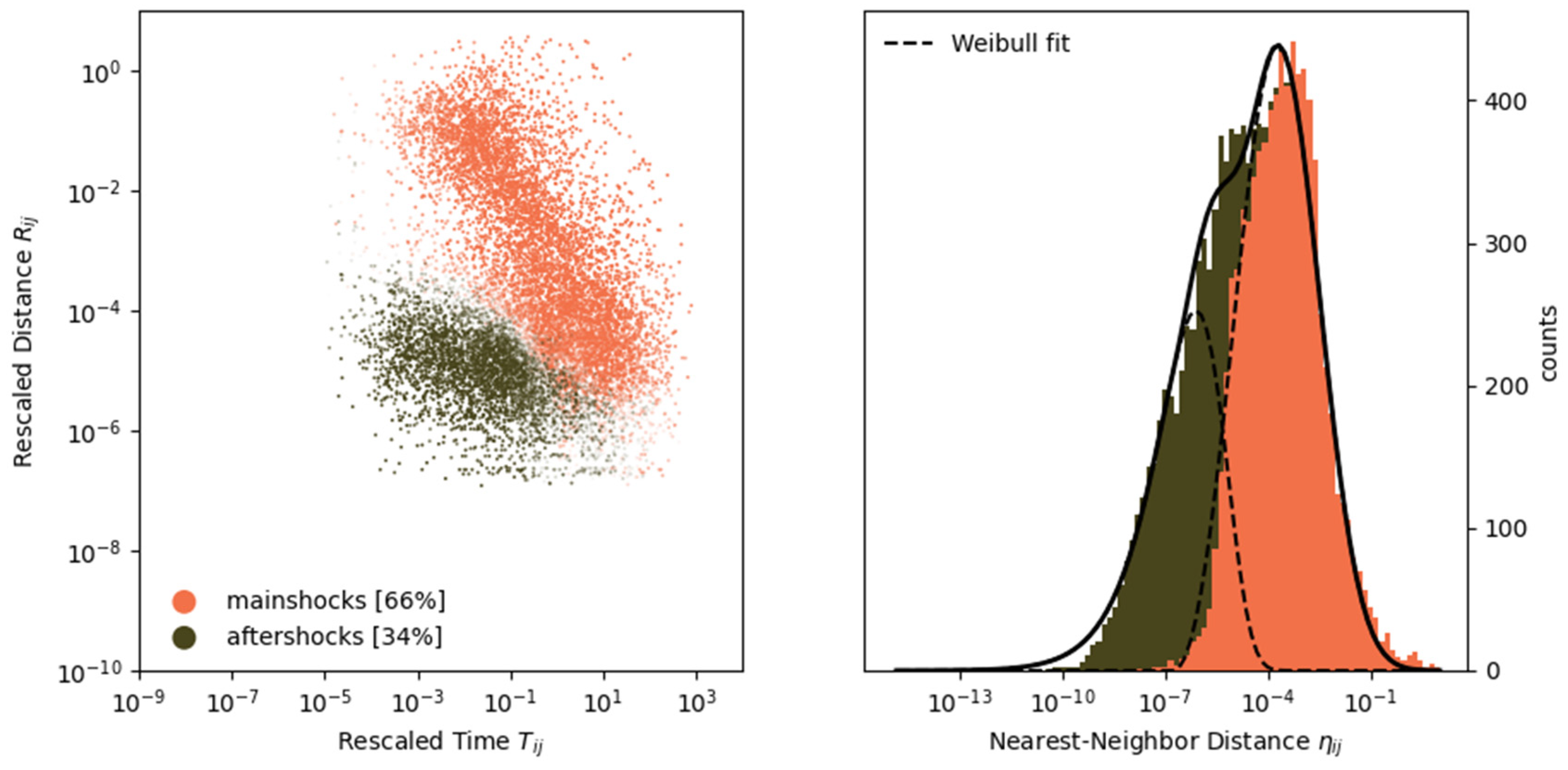
3.1. Declustering
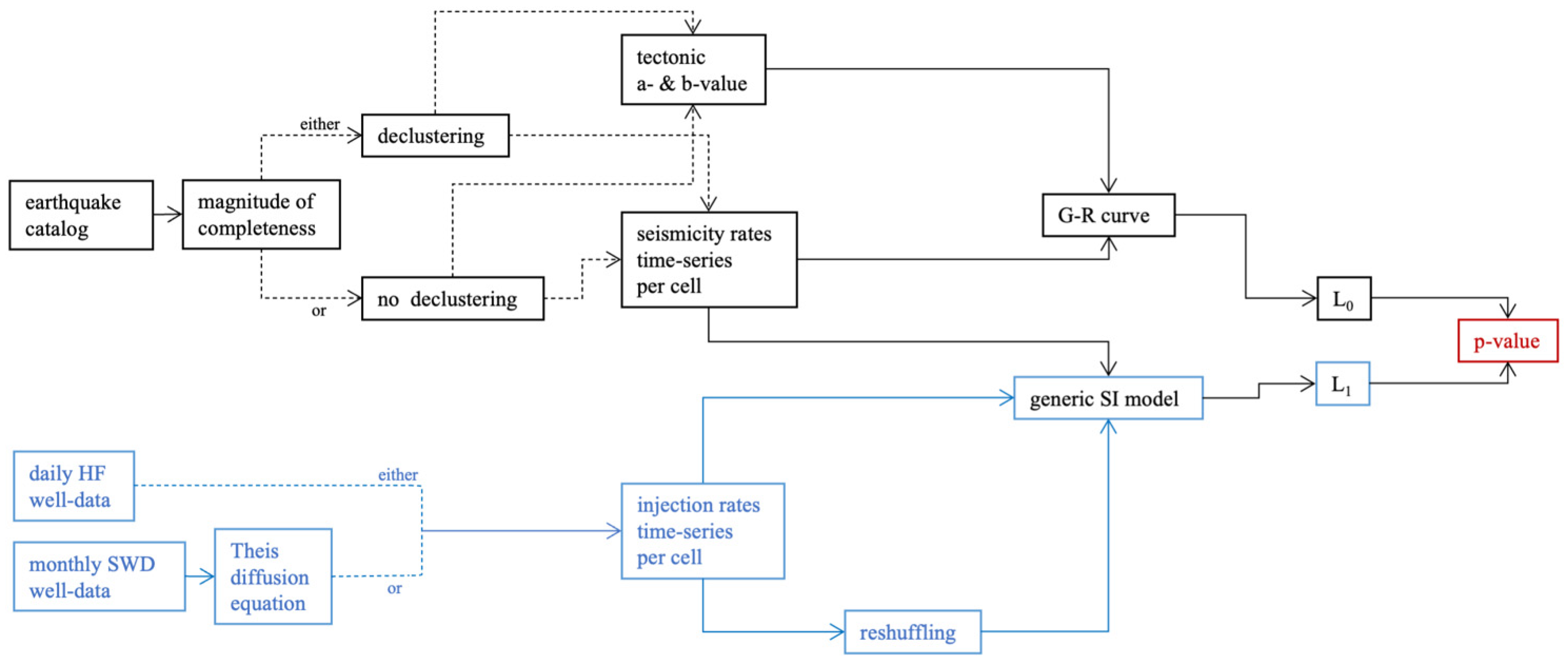
3.2. Hypotheses Testing for Causal Factors of Induced Seismicity
3.3. Generalized Seismogenic Index Model
3.4. Hydraulic Fracturing Radar
4. Results
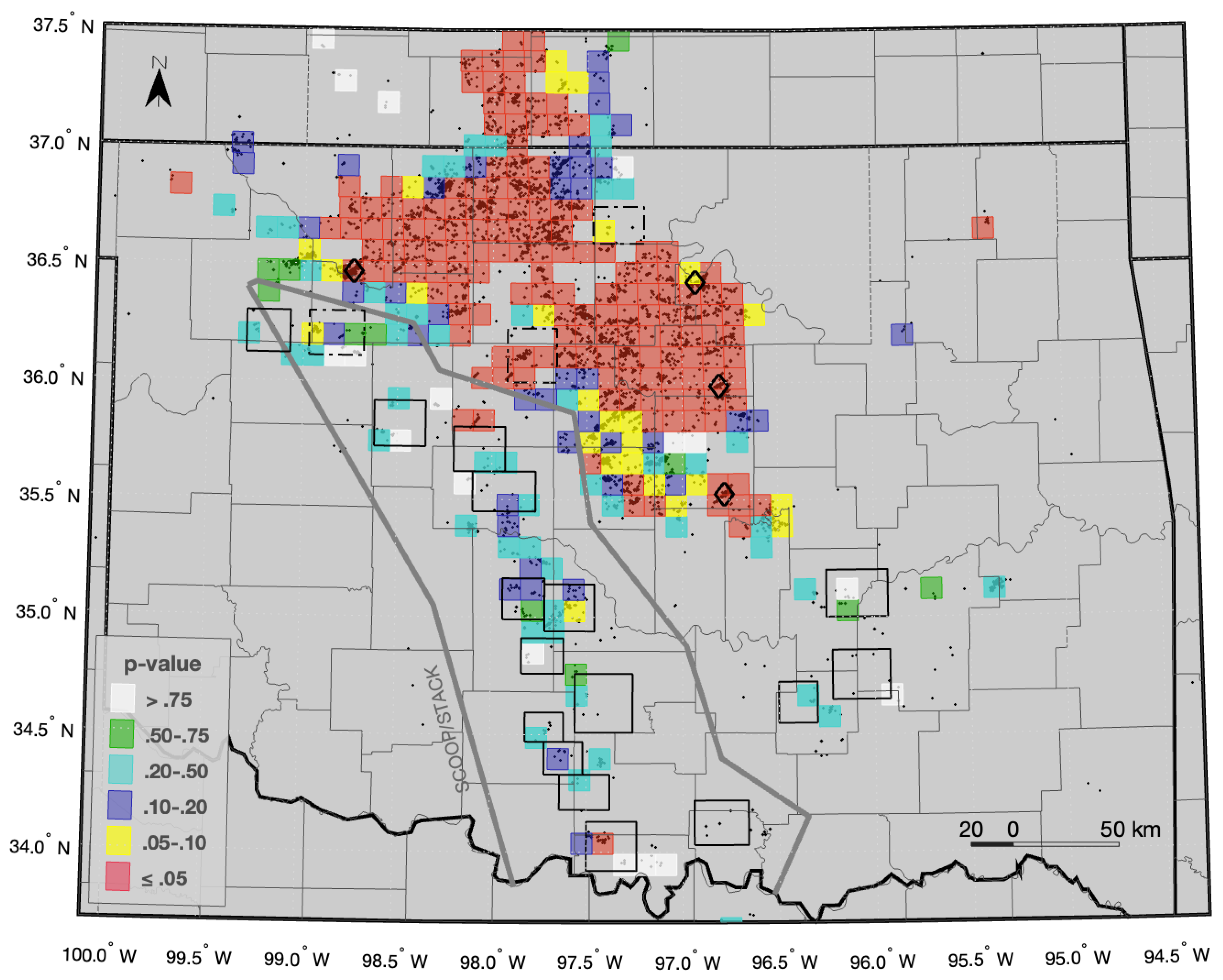
4.1. SWD
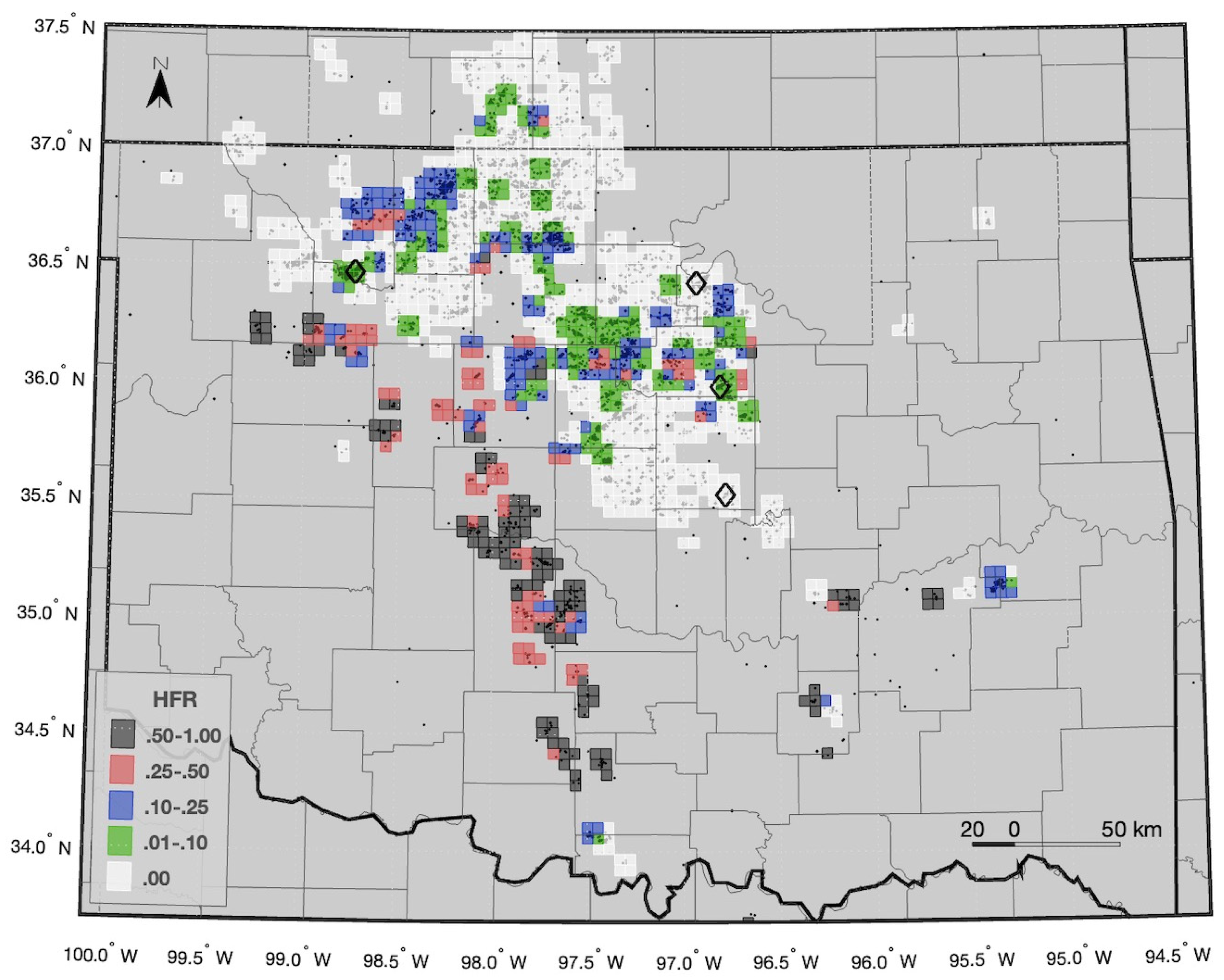
4.2. HF
5. Conclusions
Supplementary Materials
Author Contributions
Funding
Data Availability Statement
Acknowledgments
Conflicts of Interest
References
- Hough, S.E.; Page, M. A century of induced earthquakes in Oklahoma? Bull. Seism. Soc. Am. 2015, 105, 2863–2870. [Google Scholar] [CrossRef]
- Pollyea, R.M.; Chapman, M.C.; Jayne, R.S.; Wu, H. High density oilfield wastewater disposal causes deeper, stronger, and more persistent earthquakes. Nat. Commun. 2019, 10, 3077. [Google Scholar] [CrossRef]
- Weingarten, M.; Ge, S.; Godt, J.W.; Bekins, B.A.; Rubinstein, J.L. High-rate injection is associated with the increase in US mid-continent seismicity. Science 2015, 348, 1336–1340. [Google Scholar] [CrossRef]
- Langenbruch, C.; Weingarten, M.; Zoback, M.D. Physics-based forecasting of man-made earthquake hazards in Oklahoma and Kansas. Nat. Commun. 2018, 9, 3946. [Google Scholar] [CrossRef]
- Grigoratos, I.; Rathje, E.; Bazzurro, P.; Savvaidis, A. Earthquakes Induced by Wastewater Injection, Part I: Model Development and Hindcasting. Bull. Seism. Soc. Am. 2020, 110, 2466–2482. [Google Scholar] [CrossRef]
- Rubinstein, J.L.; Ellsworth, W.L.; Dougherty, S.L. The 2013–2016 Induced Earthquakes in Harper and Sumner Counties, Southern Kansas. Bull. Seism. Soc. Am. 2018, 108, 674–689. [Google Scholar] [CrossRef]
- Grigoratos, I.; Bazzurro, P.; Rathje, E.; Savvaidis, A. Time-dependent seismic hazard and risk due to wastewater injection in Oklahoma. Earthq. Spectra 2021, 37, 2084–2106. [Google Scholar] [CrossRef]
- Pollitz, F.F.; Wicks, C.; Schoenball, M.; Ellsworth, W.; Murray, M. Geodetic Slip Model of the 3 September 2016 Mw 5.8 Pawnee, Oklahoma, Earthquake: Evidence for Fault-Zone Collapse. Seism. Res. Lett. 2017, 88, 983–993. [Google Scholar] [CrossRef]
- Schoenball, M.; Ellsworth, W.L. A systematic assessment of the spatiotemporal evolution of fault activation through induced seismicity in Oklahoma and southern Kansas. J. Geophys. Res. Solid Earth 2017, 122, 10.189–10.206. [Google Scholar] [CrossRef]
- Choy, G.L.; Rubinstein, J.L.; Yeck, W.L.; McNamara, D.E.; Mueller, C.S.; Boyd, O.S. A Rare Moderate-Sized (Mw 4.9) Earthquake in Kansas: Rupture Process of the Milan, Kansas, Earthquake of 12 November 2014 and Its Relationship to Fluid Injection. Seism. Res. Lett. 2016, 87, 1433–1441. [Google Scholar] [CrossRef]
- Cochran, E.S.; Wickham-Piotrowski, A.; Kemna, K.B.; Harrington, R.M.; Dougherty, S.L.; Castro, A.F.P. Minimal Clustering of Injection-Induced Earthquakes Observed with a Large-n Seismic Array. Bull. Seism. Soc. Am. 2020, 110, 2005–2017. [Google Scholar] [CrossRef]
- Keranen, K.M.; Weingarten, M.; Abers, G.A.; Bekins, B.A.; Ge, S. Induced earthquakes: Sharp increase in central Oklahoma seismicity since 2008 induced by massive wastewater injection. Science 2014, 345, 448–451. [Google Scholar] [CrossRef]
- Keranen, K.M.; Weingarten, M. Induced Seismicity. Annu. Rev. Earth Planet. Sci. 2018, 46, 149–174. [Google Scholar] [CrossRef]
- McClure, M.; Gibson, R.; Chiu, K.; Ranganath, R. Identifying potentially induced seismicity and assessing statistical significance in Oklahoma and California. Res. Solid Earth 2017, 122, 2153–2172. [Google Scholar] [CrossRef]
- Grigoratos, I.; Rathje, E.; Bazzurro, P.; Savvaidis, A. Earthquakes Induced by Wastewater Injection, Part II: Statistical Evaluation of Causal Factors and Seismicity Rate Forecasting. Bull. Seism. Soc. Am. 2020, 110, 2483–2497. [Google Scholar] [CrossRef]
- Goebel, T.; Weingarten, M.; Chen, X.; Haffener, J.; Brodsky, E. The 2016 Mw 5.1 Fairview, Oklahoma earthquakes: Evidence for long-range poroelastic triggering at >40 km from fluid disposal wells. Earth Planet. Sci. Lett. 2017, 472, 50–61. [Google Scholar] [CrossRef]
- Chen, X.; Nakata, N.; Pennington, C.; Haffener, J.; Chang, J.C.; He, X.; Zhan, Z.; Ni, S.; Walter, J.I. The Pawnee earthquake as a result of the interplay among injection, faults and foreshocks. Sci. Rep. 2017, 7. [Google Scholar] [CrossRef]
- Norbeck, J.H.; Rubinstein, J.L. Hydromechanical earthquake nucleation model forecasts onset, peak, and falling rates of induced seismicity in Oklahoma and Kansas. Geophys. Res. Lett. 2018, 45, 2963–2975. [Google Scholar] [CrossRef]
- Holland, A.A. Earthquakes Triggered by Hydraulic Fracturing in South-Central Oklahoma. Bull. Seism. Soc. Am. 2013, 103, 1784–1792. [Google Scholar] [CrossRef]
- Skoumal, R.J.; Ries, R.; Brudzinski, M.R.; Barbour, A.J.; Currie, B.S. Earthquakes induced by hydraulic fracturing are pervasive in Oklahoma. J. Geophys. Res. Solid Earth 2018, 123, 10.918–10.935. [Google Scholar] [CrossRef]
- Ries, R.; Brudzinski, M.R.; Skoumal, R.J.; Currie, B.S. Factors Influencing the Probability of Hydraulic Fracturing-Induced Seismicity in Oklahoma. Bull. Seism. Soc. Am. 2020, 110, 2272–2282. [Google Scholar] [CrossRef]
- Ansari, E.; Bidgoli, T.S. Reply to comment by Peterie et al. on “accelerated fill-up of the arbuckle group aquifer and links to US midcontinent seismicity”. J. Geophys. Res. Solid Earth 2020, 125. [Google Scholar] [CrossRef]
- Grigoratos, I.; Savvaidis, A.; Rathje, E. Distinguishing the Causal Factors of Induced Seismicity in the Delaware Basin: Hydraulic Fracturing or Wastewater Disposal? Seism. Res. Lett. 2022, 93, 2640–2658. [Google Scholar] [CrossRef]
- Grigoratos, I.; Savvaidis, A.; Wiemer, S. Revisiting the Seismicity in the Eagle Ford Shale: The Overlooked Role of Wastewater Disposal. Seism. Rec. 2025, 5, 145–154. [Google Scholar] [CrossRef]
- Grigoratos, I.; Poggi, V.; Danciu, L.; Monteiro, R. Homogenizing instrumental earthquake catalogs—A case study around the Dead Sea Transform Fault Zone. Seismica 2023, 2, 402. [Google Scholar] [CrossRef]
- Grigoratos, I.; Wiemer, S. Probabilistic identification of seismicity triggered by oil and gas activities and its effects on seismic hazard. Final Technical Report for the USGS Earthquake Hazards Program Grant #G22AP00243. 2023. Available online: https://earthquake.usgs.gov/cfusion/external_grants/reports/G22AP00243.pdf (accessed on 1 May 2025).
- Barbour, A.J.; Norbeck, J.H.; Rubinstein, J.L. The effects of varying injection rates in Osage County, Oklahoma, on the 2016 Mw 5.8 Pawnee earthquake. Seism. Res. Lett. 2017, 88, 1040–1053. [Google Scholar] [CrossRef]
- Murray, K. Class II saltwater disposal for 2009–2014 at the annual-, state-, and county-scales by geologic zones of completion, Oklahoma. In Open-File Report: OF5-2015; Oklahoma Geological Survey: Norman, OK, USA, 2015. [Google Scholar] [CrossRef]
- Aden-Antoniów, F.; Frank, W.B.; Seydoux, L. An Adaptable Random Forest Model for the Declustering of Earthquake Catalogs. J. Geophys. Res. Solid Earth 2022, 127. [Google Scholar] [CrossRef]
- Zaliapin, I.; Gabrielov, A.; Keilis-Borok, V.; Wong, H. Clustering Analysis of Seismicity and Aftershock Identification. Phys. Rev. Lett. 2008, 101. [Google Scholar] [CrossRef]
- Shapiro, S.A.; Dinske, C.; Langenbruch, C.; Wenzel, F. Seismogenic index and magnitude probability of earthquakes induced during reservoir fluid stimulations. Lead. Edge 2010, 29, 304–309. [Google Scholar] [CrossRef]
- Shapiro, S.A. Fluid-induced seismicity; Cambridge University Press: Cambridge, UK, 2015. [Google Scholar] [CrossRef]
- Dinske, C.; Shapiro, S. Performance test of the Seismogenic index model for forecasting magnitude distributions of fluid-injection-induced seismicity. In SEG Technical Program Expanded Abstracts 2016; Society of Exploration Geophysicists: Houston, TA, USA, 2016. [Google Scholar] [CrossRef]
- Kwiatek, G.; Grigoratos, I.; Wiemer, S. Variability of Seismicity Rates and Maximum Magnitude for Adjacent Hydraulic Stimulations. Seism. Res. Lett. 2024, 96, 920–932. [Google Scholar] [CrossRef]
- Theis, C.V. The relation between the lowering of the piezometric surface and the rate and duration of discharge of a well using ground-water storage. Trans. Am. Geophys. Union 1935, 16, 519–524. [Google Scholar] [CrossRef]
- Evans, D.G.; Steeples, D.W. Microearthquakes near the sleepy hollow oil field, southwestern Nebraska. Bull. Seism. Soc. Am. 1987, 77, 132–140. [Google Scholar] [CrossRef]
- Armbruster, J.; Steeples, D.; Seeber, L. The 1989 earthquake sequences near Palco, Kansas: A possible example of induced seismicity. Seismol. Res. Lett. 1987, 60, 141. [Google Scholar]


Disclaimer/Publisher’s Note: The statements, opinions and data contained in all publications are solely those of the individual author(s) and contributor(s) and not of MDPI and/or the editor(s). MDPI and/or the editor(s) disclaim responsibility for any injury to people or property resulting from any ideas, methods, instructions or products referred to in the content. |
© 2025 by the authors. Licensee MDPI, Basel, Switzerland. This article is an open access article distributed under the terms and conditions of the Creative Commons Attribution (CC BY) license (https://creativecommons.org/licenses/by/4.0/).
Share and Cite
Grigoratos, I.; Savvaidis, A.; Wiemer, S. Seven Thousand Felt Earthquakes in Oklahoma and Kansas Can Be Confidently Traced Back to Oil and Gas Activities. GeoHazards 2025, 6, 36. https://doi.org/10.3390/geohazards6030036
Grigoratos I, Savvaidis A, Wiemer S. Seven Thousand Felt Earthquakes in Oklahoma and Kansas Can Be Confidently Traced Back to Oil and Gas Activities. GeoHazards. 2025; 6(3):36. https://doi.org/10.3390/geohazards6030036
Chicago/Turabian StyleGrigoratos, Iason, Alexandros Savvaidis, and Stefan Wiemer. 2025. "Seven Thousand Felt Earthquakes in Oklahoma and Kansas Can Be Confidently Traced Back to Oil and Gas Activities" GeoHazards 6, no. 3: 36. https://doi.org/10.3390/geohazards6030036
APA StyleGrigoratos, I., Savvaidis, A., & Wiemer, S. (2025). Seven Thousand Felt Earthquakes in Oklahoma and Kansas Can Be Confidently Traced Back to Oil and Gas Activities. GeoHazards, 6(3), 36. https://doi.org/10.3390/geohazards6030036