Earthquake History and Rupture Extents from Morphology of Fault Scarps Along the Valley Fault System (Philippines)

Abstract

The morphologic dating of single-event fault scarps along the dextral strike-slip Valley Fault System (VFS) yielded distinct clusters of relative ages (kt), which we interpret as evidence of independent surface ruptures. The boundaries between structural and geometric segments of the East Valley Fault (EVF) appear to have been nonpersistent during the recent rupture cycle. We associate the youngest cluster with the largest historical earthquake (M > 7 in 1863) felt in Manila, which is believed to have come from three segments of the EVF. Thus, future multiple-segment events, M > 7, could occur on the EVF. Our results do not support rupturing of the entire length of the West Valley Fault (WVF), but its northern segment (segment I) is capable of generating an M > 7 earthquake. This is the first time that diffusivity and relative ages of fault scarps are determined from this part of the world and is one of the few studies applying analysis of recent fault scarps to rupture segmentation studies. The recent scarps along the WVF’s segment II are due to aseismic creep and occur along pre-existing tectonic structures. Continued groundwater overextraction within the creeping zone could induce seismicity and modulate the natural timing of future earthquakes along the WVF.

1. Introduction

The 135 km long Valley Fault System (VFS) or Marikina Valley Fault System (MVFS)—an active dextral strike-slip fault with a significant dip-slip component—transects the eastern part of Metro Manila. The VFS belongs to a system of faults and subduction zones that accommodates part of the deformation due to the northwestward drift of the Philippine Sea Plate (PSP) toward the Sunda Plate (Figure 1). The VFS branches from the Philippine fault zone (PFZ)—a left-lateral strike-slip active fault that accommodates much of the relative movement of the two plates. The East Valley Fault (EVF) or East Marikina Valley Fault (EVF) and the West Valley Fault (WVF) or West Marikina Valley Fault (WMVF) are the two major segments of the VFS. Figure 1 also shows the other major active structures in the VFS region, which are believed to be influencing the deformation mechanism(s) operating in the region and the kinematics of the VFS [1,2].

Due to the close proximity of the VFS to Metro Manila and other growth centers, which are mostly underlain by soft Quaternary sediment foundation, a moderate to large earthquake occurring along these structures will strongly impact structures, utilities, and people. A large part of Metro Manila is underlain by Pleistocene volcaniclastic units derived from a volcano on the central lobe of Laguna de Bay [3], which in turn is mantled by interlayered Holocene fluvial and lacustrine sediments. The basement units consist of the Angat ophiolite of possible Cretaceous age [4] and are overlain by Upper Cretaceous pillow basalts and Tertiary sedimentary units and igneous intrusions.

Figure 1. The main physiographic and tectonic elements in central Luzon. (a) The tectonic setting of the Valley Fault System (VFS). PSP—Philippine Sea Plate, SP—Sunda Plate, PT—Philippine Trench, ELT—East Luzon Trough, and MT—Manila Trench. Direction (305° azimuth) and rate (8.0 cm/yr) of PSP motion after Seno et al. [5]. (b) The northern half of the VFS cuts across the Southern Sierra Madre, while its southern parts bound the mountain range. The East Valley Fault (EVF) branches from the PFZ, while both the EVF and the West Valley Fault (WVF) appear to terminate near the rifting front of the Macolod Corridor. Dashed lines indicate the rifting fronts while solid arrows indicate NW-SE extension of the Macolod Corridor. A preliminary assessment of VFS segmentation is also shown. Roman numerals I to X refer to the structural/geometric segments of the VFS. Sources of segmentation: [1,2].

Figure 1. The main physiographic and tectonic elements in central Luzon. (a) The tectonic setting of the Valley Fault System (VFS). PSP—Philippine Sea Plate, SP—Sunda Plate, PT—Philippine Trench, ELT—East Luzon Trough, and MT—Manila Trench. Direction (305° azimuth) and rate (8.0 cm/yr) of PSP motion after Seno et al. [5]. (b) The northern half of the VFS cuts across the Southern Sierra Madre, while its southern parts bound the mountain range. The East Valley Fault (EVF) branches from the PFZ, while both the EVF and the West Valley Fault (WVF) appear to terminate near the rifting front of the Macolod Corridor. Dashed lines indicate the rifting fronts while solid arrows indicate NW-SE extension of the Macolod Corridor. A preliminary assessment of VFS segmentation is also shown. Roman numerals I to X refer to the structural/geometric segments of the VFS. Sources of segmentation: [1,2].

Knowledge of the rupture segmentation pattern is essential to the understanding of the timing and size of near-future earthquakes along the VFS. The segmentation pattern of the VFS (Figure 1; [1,2]) was initially deduced mainly from structural, geologic, and geometric criteria. Ground ruptures, however, do not necessarily occur along only one segment. Some physical features divide fault zones into segments and control the location and extent of seismic ruptures (e.g., [6,7]). Some rupture segments persist through repeated earthquake cycles, and in some cases, rupture patterns repeat almost identically along some portions of the fault [8,9]. Other segment boundaries are nonpersistent. Wheeler and Krystinik [9], for instance, recognized the presence of persistent and nonpersistent segments along the Wasatch fault zone based on gravity, seismicity, and fault zone geometry and aeromagnetic, topographic, and structural data. Along persistent sections, ruptures are likely to occur along the same segments in the near future (perhaps in the next several millennia). Nonpersistent boundaries are less predictable in terms of rupture locations and times of activity.

The recognition and measurement of fault scarps along the VFS have been instrumental not only in mapping its segments but also in inferring its kinematics, rupture history, and rupture extents, which are essential hazard assessment parameters. The measurements of the vertical offset across scarps of all sizes and of the horizontal component of displacement along the entire length of the VFS have been significant in determining its oblique dextral strike-slip motion [1,2]. This method has advantages over other measurements (e.g., from seismic network monitoring and GPS) in resolving the kinematics and deformation history of the VFS. There is no known earthquake occurrence along the VFS based on seismological observations from which focal mechanism, rupture, and earthquake parameters can be derived. The only earthquakes ever recorded were weak shallow events (e.g., Ms 2.3 in 2014 [10] and Ms 1.1 in 2021 [11]), which are believed to have occurred near the southern terminus of segment I (see Figure 1 for the location of segment I). GPS-based studies aimed to resolve the velocity field in the VFS region. However, the velocity field in the VFS region cannot be inferred with a high degree of confidence from these studies. For example, the number and distribution of GPS stations used by Hsu et al. [12] are not sufficient to come up with reliable results. Galgana et al. [13] conclude that the “Marikina Fault” (or VFS) is undergoing significant left-lateral strike-slip motion with a component of compression at ~10–12 mm/yr, which contrasts with the findings of Rimando [1] and Rimando and Knuepfer [2] regarding its sense of motion in the late Quaternary. We would have preferred that, in Galgana et al. [13], the GPS network was denser, the velocity vectors were not gridded (interpolated, with many vectors on the surface of the sea), there were longer velocity vectors and smaller error ellipses, especially those close to the VFS, there were more velocity vectors on the west side of the VFS, and the faults/boundaries were rendered more accurately. Quality GPS data are not wrong, and interpretations from these may reflect what might be going on. Interpretations based on reliable GPS velocity vectors do not have to conform with the recent geologic deformation picture based on Holocene morphotectonic kinematic evidence. For example, some sections of an active fault may be locked.

Analysis by Rimando [1] and Rimando and Knuepfer [2] of the displacement data from offset geomorphic features suggests that the larger-scale differences in the vertical displacements and V:H ratios more likely indicate surface rupturing along the WVF and the EVF at different times involving multiple geometric/structural segments. This is also supported by the data on cumulative slip and single-event scarp heights. The offset data and the inferred rupture segmentation pattern were used in the initial assessment of the potential of the VFS for generating an earthquake with magnitude M > 7 [1,2]. However, the offset data used do not necessarily reflect the most recent pattern of faulting, as the offset data obtained from aerial photographs represent a longer-term pattern of rupturing than represented by an individual seismic cycle along the fault. The results of such assessments can be tested through trenching. Also, techniques such as the use of cosmogenic nuclides and Rare Earth Elements (REEs) in combination with structural fault data and lidar-based topographic analyses (e.g., [14,15,16,17]) have gained traction in recent years to study the number and magnitude of past earthquakes. Availability and cost considerations are the main reasons why no other dates from the VFS have become available since Nelson et al.’s [18] trenching. The estimates of the recency, recurrence, and size of pre-instrumental events along the VFS come from only one trench site that was excavated in 1995 in the northern part of the WVF’s segment I. Though it has yielded approximate dates of recent earthquake events [18], the estimate of the recurrence interval (400–600 years) may not be applicable to the other segments of the fault. Additional opportunities for trenching have been limited by the suitability of potential sites and by logistical constraints. Also, organic material is sometimes rarely preserved in fault-related stratigraphy, so alternate methods of dating recent faulting events are required. One of the many methods that have been developed for dating fault movements uses the morphology of surface fault scarps. The timing and extent of the latest earthquake events and the more likely future extent of rupture segments can be verified by studying the relative ages of the most recent single-event scarps (Figure 2). This type of study is not new to the geomorphic and paleoseismic community [19,20,21,22,23,24,25,26,27,28]. A handful of workers have applied morphologic dating to rupture segmentation studies. Work by Knuepfer [8], Turko and Knuepfer [29], and Crone and Haller [30] combined results of trenching studies with those of detailed mapping of faults and geomorphic analysis of fault scarps belonging to the Lemhi and Lost River faults to show that some rupture segments persist through repeated earthquake cycles and, in some cases, rupture patterns repeat almost identically along some portions of the fault. More recent studies [31,32,33] have also investigated fault segmentation and the behavior of rupture patterns along the Lost River Fault, further refining our understanding of how ruptures propagate across structural complexities. Dating using scarp morphology is attractive because it is cheap, fast, safe, and nondestructive [34] and can be used in at least a relative sense along the entirety of a fault [29] rather than at very few trench sites. In some cases, it may be the only dating method that can be used.

In this paper, profiles of the most recent earthquake scarps along the VFS are used to establish their relative ages. Cluster analysis is employed to examine the extent to which scarps or groups of scarps define rupture segments. The along-strike extent of rupture segments and the relative timing of recent earthquakes along individual segments are determined in a way that site-specific trenching results cannot resolve more or less continuously along strike. This study represents the first time that scarp morphologic studies have been applied in this part of the world, which has a climate and vegetation character that is quite different from those of the more common study areas in the western U.S. and other parts of the world. This is also the first time that diffusivity constant values (i.e., scarp erodibility) are generated from a tropical environment dominated by wet and dry seasons and thick vegetation cover. Also, the application of the method to understanding segmentation and the extent of seismogenic ruptures of a particular strike-slip fault system, albeit with a significant dip-slip component, is new. The knowledge gained about the timing and extent of recent rupturing from analysis of profiles should contribute to the assessment of the nature, timing, and size of past and future surface ruptures along the VFS.

2. Materials and Methods

The morphologic dating method was applied to determine the relative ages and, if possible, event ages corresponding to the most recent earthquake scarps along the VFS. The morphologic dating method is based on a simple analytical model of hillslope evolution [35], treating the scarp formed by one surface-faulting event as a small hillslope. The extent to which a slope’s initial morphology has been degraded provides the basis of morphologic dating (Figure 3).

After the formation of a fault scarp, it is rapidly degraded by processes driven primarily by gravity (e.g., slumping and spalling) until the slope attains its angle of repose. This initial stage is followed by the action of slower processes (e.g., creep and raindrop impact), which facilitate the diffusion of materials from the top toward the base of the scarp, further decreasing the slope. The development of a fault scarp during this stage can be modeled to determine the time that has elapsed since attaining its angle of repose. The diffusion dating technique is one of the techniques based on degradational processes that have been used to date fault scarps [37]. Correlations observed by Wallace [19] and Bucknam and Anderson [38] between scarp height, slope, and age paved the way for modeling of erosional degradation of fault scarps for dating earthquake events [20,34,35,39,40]. The diffusion equation was first applied in 1960 to hillslopes in general [41], and it was Nash [35] who applied it specifically to scarps. Nash’s [35,42,43] model is a linear diffusion equation and is expressed by the following equation:

dy/dt = k [(d²y)/dx²)]

where

y = elevation;

t = time since scarp reached angle of repose;

k = constant of proportionality (diffusivity);

x = horizontal coordinate of the point.

The model does not work for scarps that have not reached the angle of repose of the slope-forming materials. The model’s basic assumption that the rate of sediment transport is proportional only to the scarp slope [20] must be satisfied. This assumption requires scarp degradation mainly by creep and rain splash instead of wash processes, which increase in strength downslope. The other assumption that must be satisfied is that there should be no net addition or removal of materials to the profile. The model predicts that with time, the crestal convexity and basal concavity curvatures of a scarp profile must decrease while lateral extents increase, resulting in a gentler midsection (Figure 3). The model also assumes no overall lowering of the landscape and a constant base level for the scarp and that after the formation the scarps are left to degrade under constant conditions. The model works only for transport-limited slopes but works as well for those made of cohesionless materials dominated by soil creep. In transport-limited slopes, loose sediment is more abundant than transport processes can remove. Wallace [44] and Arrowsmith et al. ([45]; also, Arrowsmith, personal communication) cited the significant contribution of animal burrowing in making available slope materials for transport. In the study area, bioturbation by worms and ants helps supply adequate material for transport.

Some authors (e.g., [34,40,46]) have suggested that a nonlinear rather than a linear diffusion equation better fits much of the scarp data collected in previous studies. Nash’s [43] SLOPEAGE program is applied here, as it allows the use of either a linear or nonlinear diffusion model [47]. The validity of the linear diffusion model with the VFS data set will be tested. SLOPEAGE’s appeal lies in its ability to determine the best morphologic age for the entire profile or for any portion of it. It may be used for any midsection slope angle less than 90°, in contrast to the nonlinear model of Andrews and Bucknam [34], which is applicable only in the lower angle ranges (10–24°) and does not assume that the base and crest of the scarp are parallel slopes unless the user specifies that they are to be set parallel. In addition, SLOPEAGE yields an r² (RMS) measure of “goodness of fit” between the best-fit model profile and the observed profile (original field data). The method determines the relative age, kt, which is the product of the diffusivity (k) and morphologic age (t). The diffusion coefficient or diffusivity (k) indicates the rate of transport of sediment (in m²/y) after a scarp attains its angle of repose. The morphologic age (t) is the time elapsed (in years) since the scarp reached its angle of repose. Below are the steps described by Nash [35,42,43] for the morphologic dating of scarps. Refer to Figure 4 for the parameters used in the procedure.

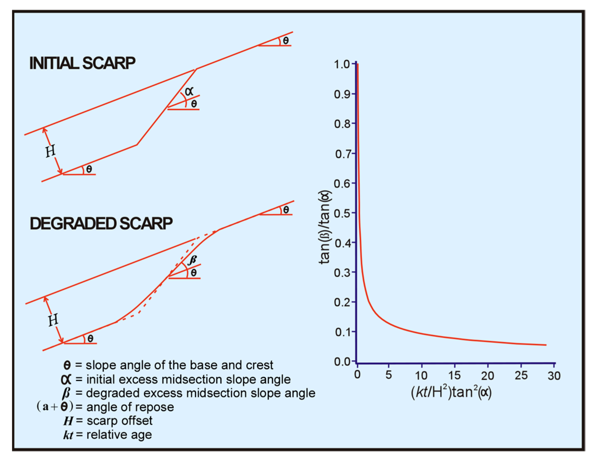
• Step 1: Determine H, β, and θ from a detailed profile of the scarp. (H = scarp offset; β = degraded excess midsection slope angle; θ = slope angle of the crest and base). See the left part of Figure 4 for these parameters.
• Step 2: Determine α, the initial excess midsection angle, either directly or indirectly, by measurement of the angle of internal friction, Φ (or angle of repose = α + θ), of the material underlying the scarp. α is equal to the difference between the angle of repose and slope of the crest and base (θ). The value of (α + θ) is equivalent to the angle of repose.
• Step 3: Calculate tan(β)/tan(α) and use it to determine the corresponding value of (kt/H²)tan²(α) from the curve (see right part of Figure 4) describing the relationship between the initial excess midsection slope angle, α; the degraded excess midsection slope angle, β; the scarp offset, H; the hillslope diffusivity, k; and the age of the hillslope, t.
• Step 4: Calculate relative age, kt, by multiplying (kt/H²)tan²(α), determined in step 3, by H²/tan²(α), calculated from the values of H and α found in Steps 1 and 2.
• Step 5: If t is known and k is to be calculated, determine k by dividing kt, found in Step 4, by t. If k is known and t is to be calculated, determine t by dividing kt, found in Step 4, by k.

The process of degrading toward the angle of repose may take a few tens to perhaps a thousand years in the western U.S. [19,48,49] but may take only, at most, decades in places like New Zealand or the Philippines, except where roots armor the scarp so thoroughly that gravitational failure is inhibited [Knuepfer, personal communication]. Aside from the climate, slope aspect, and associated vegetation, the lithologic properties of the scarp material, such as grain size and cohesion, also affect the rate of diffusion [42,50]. Although Dodge and Grose [51] noted higher degradation rates in clay compared to gravel, noncohesive sands are known to degrade faster than poorly sorted, slightly cohesive fan gravel [50]. When diffusivity (k) values from a wide range of conditions (e.g., climate, hillslope aspect, and scarp material) become available, t can be estimated using procedures for morphologic dating (e.g., [35,42,52]).

For this study, the morphologic age (t) is considered less important at this point than the measure of the relative age, kt. For reasons discussed earlier, there are no absolute ages available from the most recent fault scarp sites. This is also the first time that degradation rates of fault scarps from any place in the Philippines have been determined. Thus, neither k nor t can be obtained a priori. However, we rely on historical accounts of earthquakes from VFS to estimate the erosion constant (diffusivity), k.

The diffusivity constant derived in this paper is the first of such determinations in a tropical setting. Results of the k determination will be compared with those from different regions as summarized by Nash [43], Arrowsmith et al. [45], and Hanks [53].

A total of 52 scarp profiles were gathered from 28 different sites along the segments of the VFS (Figure 5). Whenever possible, more than one profile was measured for each site. Many of these scarps had been identified in the aerial photos prior to actual field measurement. Scarp profile sites are absent or lacking along some portions of the VFS. Field studies and aerial photo interpretations also yielded no recent scarps from three segments (segments X, VII, and VIII; Figure 5). A real lack of the vertical component of displacement and nonpreservation accounts for the absence of scarp profile sites in some places. Rapid urbanization partly accounts for the loss of scarps along some parts of the VFS. Logistical considerations (including permission, lack of roads, and rebel activity) also limited accessibility to some areas. All profiles collected most likely represent single-event scarps based on comparison with vertical offsets from the 1991 Luzon and 1994 Mindoro earthquake ruptures (mostly within the 0.5 to 2 m range). Since scarps of more than a few meters are rare, these are excluded from the analysis. Only single-event scarps can be dated by the technique used, as applying the method to fault scarps formed by multiple surface-rupture events will yield an age that is too great for the youngest event but too young for the oldest event represented. Multiple-event scarps are excluded by profiling and modeling only the steepest portion of the slope, the upper original scarp surface (between the original and rejuvenated scarp crests), and the lower original scarp surface.

This study will attempt to discriminate if kt values cluster along the fault and assign corresponding event ages to each cluster (if there is more than one cluster) to come up with estimates of diffusivity. This study seeks to verify the extent of the more recent surface rupture(s) along the VFS and whether segment boundaries (established mainly through structural, geologic, and geometric criteria) have been persistent or not.

3. Results and Discussion

3.1. Relative Age Estimates

Estimating relative ages from scarp profiles using Nash’s [43] SLOPEAGE requires information on angles of repose. The method prescribed by Morisawa [54] was followed for the determination of angles of repose from samples of scarp material from each of the profile sites. The angles of repose that we have obtained (

Table 1. Angles of repose of scarp-forming materials.

Sample	Mean	Standard Deviation	Site Mean
8A	44.2	1.8	44.8
8B	45.3	3.4	44.8
9A	43.3	1.8	44.0
9B	45.4	1.4	44.0
9C	43.2	1.7	44.0
10	50.4	2.9	50.4
12	61.3	2.2	61.3
13	47.5	2.1	47.5
15	56.3	4.3	56.3
16	47.4	2.1	47.4
17A	60.6	2.1	59.8
17B	59.0	2.7	59.8
18	49.4	1.9	49.4
19A	47.2	2.8	45.7
19B	44.2	2.0	45.7
20A	50.6	2.9	50.0
20B	49.4	1.9	50.0
21	47.2	2.2	47.2
22	45.7	3.0	45.7
23A	44.8	2.0	46.0
23B	47.3	2.7	46.0
23C	N.D.	N.D.	N.D.
24A	44.2	2.4	47.6
24B	50.9	1.5	47.6
24C	N.D.	N.D.	N.D.
25A	44.8	1.1	46.9
25B	41.7	1.5	46.9
25C	54.3	2.7	46.9
26A	54.3	3.2	53.3
26B	50.8	2.8	53.3
26C	54.7	3.0	53.3
27A	56.6	4.3	56.1
27B	55.6	3.7	56.1
28A	52.9	3.7	54.8
28B	56.6	3.6	54.8
29A	49.2	3.6	53.2
29B	57.3	2.4	53.2
31A	58.7	2.3	56.0
31B	53.3	3.8	56.0
32A	49.8	4.1	48.5
32B	47.3	2.6	48.5
35	47.4	1.9	48.6
37A	50.3	3.0	50.1
37B	49.9	2.1	50.1
40A	56.4	4.3	52.2
40B	48.1	3.4	52.2
41A	49.2	3.5	49.2
41B	49.2	3.5	49.2
42A	42.2	1.6	43.0
42B	43.8	2.2	43.0
43A	44.8	2.0	46.1
43B	47.4	2.7	46.1

) using the method range in value from around 42.5° (site 42) to around 60° (site 12). The high values obtained, which are consistent with some field observations, are attributed to the high clay content of the poorly sorted samples that provide high cohesive strength to the sediments.

Figure 6 shows the results of applying Nash’s [43] SLOPEAGE program to selected profiles from segments where recent scarps had been mapped.

Table 2. Summary of relative age estimates and scarp morphology parameters.

Segment	Site	Dist.	Offset	kt *	r2 †	Andrews Hanks
		(km)	(m)	(m2)		(tk) §
I	8A	64.1	2.44	1.43	0.9626	1.54
	8B	64.1	3.42	2.02	0.9898	1.87
	9A	64.8	1.16	2.17	0.9757	2.02
	9B	64.8	0.91	1.12	0.9296	2.90
	9C	64.8	0.55	0.14	0.9922	0.38
	10	63.6	2.92	1.17	0.9945	1.22
III	20A	15.5	1.36	0.56	0.9595	0.49
	20B	15.5	0.90	0.99	0.8863	0.96
	19A	16.1	0.81	0.42	0.9866	0.42
	19B	16.1	0.68	0.50	0.9849	0.69
	12	16.8	1.05	0.31	0.9924	0.36
	25A	17.3	1.38	1.30	0.9770	1.24
	25B	17.3	2.25	1.76	0.9739	1.58
	25C	17.3	0.67	0.44	0.9761	0.57
IV	41A	0.7	1.65	0.21	0.9914	0.27
	41B	0.7	1.19	0.15	0.9926	0.21
	42A	0.9	0.95	0.15	0.9961	0.22
	42B	0.9	0.47	0.04	0.9995	0.14
	43A	1.0	0.85	0.50	0.9935	0.59
	43B	1.0	0.97	0.55	0.9924	0.59
	24A	3.9	0.82	0.48	0.9927	0.42
	24B	3.9	1.03	0.10	0.9963	0.10
	24C	3.9	1.44	0.74	0.9868	0.67
	23A	5.3	0.83	0.17	0.9842	0.17
	23B	5.3	1.00	0.10	0.9799	0.11
	23C	5.3	1.11	0.54	0.9907	0.57
	22	6.5	1.21	1.33	0.9590	1.15
	21	7.7	1.77	0.46	0.9804	0.46
V	31A	122.5	0.53	0.08	0.9867	0.24
	31B	122.5	0.30	0.17	0.9957	0.51
	26A	125.3	1.99	1.04	0.9135	1.02
	26B	125.3	3.38	0.89	0.9766	0.87
	26C	125.3	3.12	1.01	0.9443	0.88
	27A	127.3	0.81	0.39	0.9950	0.58
	27B	127.3	0.39	0.20	0.9990	0.50
	28A	127.8	N.A.	0.10	0.9989	N.A.
	28B	127.8	N.A.	0.19	0.9964	N.A.
	29A	130.8	2.00	0.20	0.9821	0.33
	29B	130.8	1.85	0.03	0.9737	0.19
VI	16	64.5	1.90	0.50	0.9424	0.48
	18	65.2	N.A.	0.06	0.9805	N.A.
	17A	65.8	1.49	0.18	0.9732	0.16
	17B	65.8	0.93	0.04	0.9970	0.05
	40A	66.7	1.71	0.40	0.9783	0.39
	40B	66.7	0.68	0.27	0.9931	0.32
	15	69.1	N.A.	0.43	0.9953	N.A.
	13	69.5	1.06	0.01	0.9841	0.03
IX	32A	43.8	1.22	0.77	0.9828	0.88
	32B	43.8	0.39	0.34	0.9637	0.69
	35	50.5	0.22	0.03	0.9825	0.13
	37A	50.6	0.75	0.19	0.9950	0.32
	37B	50.6	0.68	0.18	0.9796	0.26

* Product of degradation constant k and time t since scarp reached the angle of repose. † Goodness of fit from degradation modeling. § Morphologic age using Andrews and Hanks [55] inverse solution method.

shows the relative age (kt) and corresponding r² for all profiles from the sites shown in Figure 5. Relative ages (kt) are also shown in a plot of kt vs distance in Figure 7. As discussed in the preceding sections, morphologic dating is not without uncertainties. Model errors due to the effects of scarp height, climate, slope aspect, time, vegetation, and lithology [50,53] may result in variations in the degradation constant (k) and thus variations in the relative age (kt). Values of kt from scarps on individual geomorphic surfaces (Table 2) vary by as much as 100%. Therefore, kt values must differ greatly to be considered for different ages. Individual sampling sites are generally quite close to adjacent sites, but groups of sampling sites are not. This large separation between groups (several kilometers to tens of kilometers) was used as an initial basis for designating the derived relative age or kt (Table 2; Figure 7) for each site into ad hoc clusters. The locations of the ad hoc clusters coincide with the segment positions. To determine the distinctness of each cluster or groups of clusters, t-tests of kt cluster means were carried out (

Table 3. Results of t-tests of the mean of kt for each cluster.

Segments	Distance	Mean kt	Stdev.	Sample	t Score	t Range
				Size		0.01 Level	0.05 Level
I and III
I	63.6 to 64.8	1.34	0.73	6
III	15.5 to 17.3	0.79	0.52	8
					−1.54	−3.06 to 3.06	−2.18 to 2.18
III and IV
III	15.5 to 17.3	0.79	0.52	8
IV	0.7 to 7.7	0.39	0.35	14
					−2.02	−2.84 to 2.84	−2.09 to 2.09
I and IV
I	63.6 to 64.8	1.34	0.73	6
IV	0.7 to 7.7	0.39	0.35	14
					3.72	−2.88 to 2.88	−2.10 to 2.10
I and VI
I	63.6 to 64.8	1.34	0.73	6
VI	64.5 to 69.5	0.24	0.19	8
					3.79	−3.06 to 3.06	−2.18 to 2.18
V and VI
V	122.5 to 130.8	0.39	0.39	11
VI	64.5 to 69.5	0.24	0.19	8
					−0.98	−2.9 to 2.9	−2.11 to 2.11
I and V
I	63.6 to 64.8	1.34	0.73	6
V	122.5 to 130.8	0.39	0.39	11
					3.28	−2.95 to 2.95	−2.13 to 2.13
I + III + IV and VI
I + III + IV	0.7 to 64.8	0.71	0.61	28
VI	64.5 to 69.5	0.24	0.19	8
					−2.11	−2.73 to 2.73	−2.03 to 2.03
VI and IX
VI	64.5 to 69.5	0.24	0.19	8
IX	43.8 to 50.6	0.30	0.28	5
					−0.46	−3.11 to 3.11	−2.2 to 2.2
V and IX
V	122.5 130.8	0.39	0.39	11
IX	43.8 to 50.6	0.30	0.28	5
					0.43	−2.98 to 2.98	−2.14 to 2.14
I + III + IV and V + VI + IX
I + III + IV	0.7 to 64.8	0.71	0.61	28
V + VI + IX	64.5 to 130.8	0.32	0.31	24
					2.78	−2.68 to 2.68	−2.01 to 2.01

). Our results indicate that, with the exception of segments I and IV, there are no significant differences between the mean relative ages (kt) of scarps from all pairs of WVF’s segments at both the 0.01 and 0.05 significance levels. The mean kt of scarps from all pairs of EVF’s segments also do not differ significantly at both the 0.01 and 0.05 significance levels. The differences between the mean relative age of EVF segment V scarps and WVF segment I scarps, and between the overall mean kt of WVF and EVF, are significant at both the 0.01 and 0.05 significance levels. These results support the interpretation that the rupturing of EVF involves multiple segments and is independent of the timing of the rupturing of the WVF or its segments. This interpretation assumes that diffusivity values for EVF and WVF scarps are approximately the same. The EVF scarps face west and the WVF scarps face east. Differences in the slope aspect have been known to cause differences in diffusivity values [40]. However, it is not certain to what degree differences in slope aspect affect diffusivity values of the EVF and WVF scarps.

Interpreting the timing and extent of ruptures along the WVF is less straightforward. The mean relative age of segment III is less than that of segment I but greater than that of segment IV (Table 3). The mean kt for segment III is not significantly different from the mean relative ages (kt) of segments I and IV. However, the mean relative ages (kt) for segments I and IV are significantly different from each other at both the 0.01 and 0.05 levels. One possible interpretation is that segments I, III, and IV ruptured at different times, with the earthquake that ruptured segment III intervening between the events that ruptured segments I and IV. Another possible interpretation is that, during one of the more recent earthquake events, segment III ruptured in combination with parts of segments I and IV. In either case, the interval time between the rupturing events must have been shorter than the intervening time between events that ruptured segments I and IV. Another complicating issue is the observed tapering off of net displacements toward both ends of the WVF portion between the 0 and 50 km marks [1,2]. These kinds of slip deficits near the ends of segments have been interpreted by Wheeler [7] as the result of many large earthquake ruptures terminating near these zones. If the most recent rupture pattern of the southern portion of the WVF is similar to the long-term pattern, then the slip deficit observed favors the most recent rupturing along the combined segments IV and III (and part of segment I).

3.2. Diffusivity and Morphologic Ages

The linear diffusion model’s assumption that the rate of sediment transport is proportional only to the scarp slope requires that the relative age (kt) should be independent of the scarp offset [40,47]. How this relationship applies to the VFS scarp offset and relative age data (Table 2) is tested through a plot of scarp height vs. relative age for EVF (Figure 8a) and WVF (Figure 8b). Best-fitting regression lines were derived from these plots. For the EVF cluster, there is no clear relationship between the relative age and height of lower scarps (Figure 8a). Though relative age generally increases with increasing scarp height, the low degree of this dependence is indicated by the gentle slope of the regression line (Figure 8a). By excluding more of the outliers, the relationship shifts to a more constant kt with respect to the scarp height. The effect of the scarp height on the relative age may be due to transport by slopewash, which increases in effectiveness as the height and length of the slope increase [39,50]. Because the scarp height influences the relative age to some degree, kt values were calculated for the EVF cluster from the best-fitting regression line (Figure 8a) by normalizing to 2 m scarp offsets (

Table 4. Summary of diffusivity and age estimates.

Segment	Mean kt	Stdev.	Age	k	Stdev.	Age	Stdev.	ktnor § (m2)	knor † (m2/kyr)
	(m2)	(m2)	(Years)	(m2/kyr)	(m2/kyr)	(Years)	(Years)	to 2 m	to 2 m
EVF
VI	0.30	0.28	-	ND	ND	ND	ND	-	-
IX	0.24	0.19	-	ND	ND	ND	ND	-	-
X	0.39	0.39	-	ND	ND	ND	ND	-	-
X + IX + VI	0.32	0.31	~130 *	2.47	2.39	-	-	0.53 ± 0.25	4.07 ± 1.92
WVF
I	1.34	0.73	-	2.47	2.39	544	604	-	-
III	0.79	0.52	-	ND	ND	ND	ND	-	-
IV	0.39	0.35	-	2.47	2.39	160	209	-	-
I + III + IV	0.71	0.61	-	2.47	2.39	ND	ND	-	-

*: based on profile data taken 25 years ago. ^§: Normalized relative age. ^†: Normalized diffusivity.

). The use of this scarp height will allow comparison of k values from the VFS region with those from other parts of the world. The normalized kt value is 0.53 m² for the EVF cluster (Table 4). We did not estimate normalized kt values for individual WVF segments because the number of scarps for each is too small. The mean kt values for the EVF and WVF scarp clusters shown in Table 4 were directly calculated from the kt values of the scarps. The estimated mean kt of EVF scarps is 0.32 ± 0.31. Higher values were obtained for the scarps of segments I, III, and IV (Table 4) from the WVF.

Since no direct measurement of diffusivity for the study area is available, the record of written historical accounts was examined for any hint regarding the age of recent faulting, if any, along parts of the VFS. This age will be used to estimate diffusivity for the younger (EVF) cluster, which in turn, can be the basis for calculating the age of the older cluster. The historical record of Philippine earthquakes is over 400 years from both written accounts (since 1589) and the instrumentally derived seismic database covering ~100 years. Since the first account of an earthquake from Manila (1599), numerous other earthquakes have affected the city (e.g., 1601, 1658, 1700, 1766, 1771, and 1863; Repetti [56]; Garcia et al. [57]; Bautista [58]). The 1601, 1658, 1771, and 1863 earthquakes were the strongest in Manila that could possibly be linked to the VFS. Accounts of damage due to most of these earthquakes are too localized to link them with certainty to the VFS. The 1863 earthquake is the one exception.

The locations of the 1863 and other earthquakes have been inferred from isoseismal maps [58,59]. According to Bautista [58] and Bautista and Oike [60], the source of the 1863 event is close to the city of Manila and falls almost on top of the hypothesized southeastern extension of the east Zambales fault on the eastern shore of Manila Bay (see isoseismal map for the 1863 event in Bautista [58]). We have reviewed written accounts for the locations of damaged areas (Figure 9) based on Repetti’s [56] compilation and Bautista’s [58] tabulation of damaged areas. Our analysis suggests the VFS is the more likely source of the 1863 earthquake. Most of the affected localities are near the Manila Bay shore areas of soft Quaternary cover. There was no damage reported from areas of thick Quaternary sediments on the western side of the east Zambales fault or from the region north of Lubao and Bacolor (Figure 9). Several towns were already in existence at the time of the earthquake in these areas [58], so these towns most likely received no or minor damage. Therefore, we conclude that the youngest VFS event documented by the youngest scarps of the EVF occurred in 1863.

If a period of about a decade is assumed as the time it takes for scarps in the region to attain the angle of repose, then 130 years is taken as the morphologic age of the most recent scarps of the eastern segments of the VFS. We use this age to estimate the diffusivity constant. This yields a diffusivity constant value of 4.07 m²/kyr for a 2 m scarp based on a normalized kt value of 0.53 m² (Table 4). Compared with most k values in other regions of the world [45,47,53], our results are relatively high. Values of k obtained from different parts of the world range from 0.1 to 16 m²/kyr [45,53]. The differences in k values between regions are attributed primarily to differences in climate, though vegetation, grain size, lithology, and slope aspect influences have also been documented [45,50,53]. The effect of the slope aspect is to vary microclimate conditions [50]. The lowest values (0.1 m²/kyr) come from Israel, which has an extremely arid climate [24]. Higher values of ~1 m²/kyr have been derived from the semi-arid region of the western United States. The highest values of k (up to 16 m²/kyr) were obtained from the relatively wet Santa Cruz Mountains, California area [20,45]. Arrowsmith et al. [45] quoted an annual precipitation ranging from ~18 cm/yr in central California to ~48 cm/yr in the San Francisco Bay area. They obtained a k of about 8.5 m²/kyr from the Carrizo Plain, where the materials are mainly poorly consolidated, moderately sorted medium sands with occasional pebble to cobble stringers. Comparable k values were obtained from Michigan in a region of high precipitation and unconsolidated materials [53]. Hanks [53] proposed that the denser vegetation in Michigan was an offsetting factor. The high precipitation (~200 cm/yr) in the VFS region partly explains the relatively high value of k that we have obtained. It is not as high as the highest k values that have been derived elsewhere, probably due to thick vegetation that slows down slope degradation [53]. Lithological properties, such as relative coarseness, poor sorting, and cohesiveness, most likely, are also important.

Assuming that the diffusivity of the EVF and WVF scarps are approximately the same, the morphologic ages of the WVF segments can be estimated. From the mean kt values shown in Table 3 and Table 4, we obtain morphologic ages of 545 ± 600 years and 160 ± 210 years for the scarps of segments I and IV, respectively. The youngest event recognized by Nelson et al. [18] from a trench in the northern part of segment I cut a debris flow deposit that was deposited after A.D. 1420–1630 [18]. The earthquake that is associated with the segment I scarps could be the 1601 or 1658 event or an event that occurred before the first accounts of earthquakes in the Philippines. The segment IV scarps most likely correspond with either the 1658 or 1771 earthquake.

3.3. Aseismic Creep Scarps and Implications on Timing of Future Coseismic Events

3.3.1. Nature, Age, and Slip Rates

Up until now, we have discussed only the coseismic scarps found interspersed with other morphotectonic features along the various segments of the VFS. Aseismic creep scarps (Figure 10a–c), which by far are the most dominant geomorphic features along segment II, have been actively forming due to the ongoing aseismic creep. These follow old multi-event scarps, which are believed to be tectonic in origin [1,61].

The creeping ground ruptures are not irregular random fissures but fall under the surface fault type of aseismic ground failure [62,63]. Creep occurs along 15 NE–SW-trending faults arranged en-echelon within a 15 km-long and 1.5 km-wide zone (segment II of the VFS) within the dilational gap between the right-stepping segments I and III of the WVF (Figure 11) [1,2,61,64]. Previous works [1,61,64] identified groundwater withdrawal as the more likely trigger of accelerated creep primarily because of the high rates of slip that have been recorded since the 1990s, which are higher than the known tectonic creep rates [65,66,67,68,69,70,71]. Slip rates at selected sites had been estimated from scarp heights as determined from profiles generated through precise leveling (Figure 11) and the age of offset references (e.g., roads). Though there is uncertainty regarding the time of initiation of rupturing within the creeping zone, the occurrence of creep was first reported in the early 1990s [1,61,64]. The first and longest ground rupture was mapped in the northernmost part of the creeping zone (Figure 11) on 21 July 1994 [1,61,64]. Slip rates had been much higher in the 1990s (as high as 20 cm/y) [1,61,64] when a sharp rise in displacements coincided with substantial increases in the amount of groundwater extraction [64]. It remains high (2–3 cm/y) to this day in the southern part of the creeping zone, which is not covered by the 2004 groundwater extraction ban by the National Water Resources Board (NWRB) [64]. These rates are much higher than the geological slip rate of the VFS (5–7 mm/yr) [1].

3.3.2. Possible Implications of Continued Creep: Induced Seismicity and Modulated Timing of Seismicity Along VFS Segments

In contrast to the coseismic scarps that we have described, the scarps along segment II are aseismic in nature and were triggered by groundwater withdrawal. Seismicity may be induced by continued groundwater extraction within the creeping zone as argued by Rimando et al. [64] based on examples of occurrences worldwide [72,73,74,75,76,77,78]. They have discussed theories explaining the mechanism of fault failure and earthquake generation by depressurization due to fluid extraction [74,75,76,77,78,79]. Rimando et al. [64] also explored the possibility of earthquakes resulting from creep [80]. The occurrence of creep-related earthquakes may be related to the development of resistors to slip [80,81,82,83,84,85] as barriers and asperities [86,87,88,89], which manifest as step-overs and bends along the surface fault trace. Sudden fault failure could extend beyond the creeping zone. As the creeping zone corresponds to a dilational jog and an obstacle to slip transfer, it may eventually become a site of rupture initiation [90,91,92]. Its failure by continued depressurization could induce static stress changes that may lead to the failure of segment I or segment III [61,64]. The weakening of such a barrier could also facilitate contagion during an earthquake originating along either of the adjacent segments. Thus, the timing of future earthquakes along the WVF may be modulated by continued overextraction of groundwater and aseismic creep along segment II.

4. Summary and Conclusions

In spite of the large range in our kt values, suggestive of the departure of the VFS scarp data from the linear diffusion model, we were able to distinguish distinct groups of scarps by taking advantage of the large separation between the groups’ relative ages. The youngest of these sets of scarps are the EVF scarps and are likely associated with the 1863 earthquake event. Two other distinct kt clusters of VFS scarps are identified with the northernmost (segment I) and the southernmost segments (segment IV) of the WVF. A third rupture segment that involves segment III possibly overlaps both segments I and IV. There are other possible interpretations, but we cannot precisely resolve the extent and timing of this rupture segment. The earthquake that may be associated with the segment I scarps could be the 1601 or 1658 event felt in Manila or a pre-1601 event. The segment IV scarps could be associated with either the 1658 or 1771 event but are more likely associated with the 1771 earthquake. Thus, the results of our study on young VFS fault scarps suggest segmented behavior of the VFS during its most recent rupture cycle, at least within the resolution of the scarp data. The most recent rupturing along the EVF involved multiple segments. While there is a sufficiently large separation between the timing of rupturing associated with the scarps of segments I and IV, we are uncertain about the extent of the individual ruptures.

Rupture along the EVF involving multiple segments inferred from the study of the most recent scarps supports earlier findings [1,2] of the EVF’s potential for generating an M > 7 earthquake based on the combined length of its segments and on the maximum scarp height found. The maximum magnitude of earthquakes along the EVF based on scarp height (~M7.5) [1,2] is consistent with the magnitude estimated from its length. The study of single-event fault scarps, however, does not support rupturing of the entire length of the WVF. Nevertheless, the northern segment of the WVF is capable of generating an M > 7 earthquake. The probable magnitudes of future earthquakes along the southern WVF (M6 to M7) are constrained by the shorter lengths of the rupture segments. Segment I is the most likely VFS segment to generate a moderately large earthquake in the near future based on what we currently know (however limited) about the recurrence of any VFS segment and on the timing of the latest large earthquake along it from our scarp study.

Our findings about the nature and control of creep along segment II should also be considered in assessing future earthquake hazards from the WVF. Recent scarps along segment II are aseismic in nature and have been generated by creep displacement along pre-existing tectonic structures. Creep was triggered and has been controlled by groundwater extraction. If it remains unabated, continued overextraction of groundwater, especially in the southern part of the creeping zone, will exacerbate the effects of vertical creep on man-made structures. With continued overextraction of groundwater, the occurrence of induced seismicity within the creeping zone may result. The weakening of pre-existing coseismic faults within the creeping zone could lead to the modulation of the natural timing of earthquakes along nearby segments of the WVF. However, it should be emphasized that continued overextraction of groundwater does not always directly trigger an earthquake. Moreover, the triggering and timing of any earthquake along the adjacent segments depend on the resistance of a barrier to stress and the transfer of an additional stress load from one segment to another and on the physical state of the target segment of the transfer, which is unknown. Nevertheless, the potential for triggering earthquakes by continued groundwater extraction should be considered in planning for contingencies.

The diffusivity constant associated with the EVF (4.07 m²/kyr for a 2 m scarp) is relatively high compared with most of the reported diffusivity constants from studies elsewhere in the world. However, this diffusivity value is not as high as those obtained from unconsolidated sediments in relatively wet regions (up to 16 m²/kyr), in spite of exposure to heavy precipitation from monsoon rains and tropical cyclones. This is more likely due to the retardation of nonlinear processes such as slopewash by relatively dense vegetation cover and to other factors such as grain size, sorting, and cohesion (the latter of which is reflected in the high angles of repose obtained in this study).

This study represents the first time that the relative ages of fault scarps have been determined in this part of the world, and it is one of the few studies applying analysis of recent fault scarps to rupture segmentation studies. This study also represents the first determination of diffusivity in this part of the world. Despite all the reservations about dating using scarps, including our lack of understanding of slope processes and other sources of uncertainty, this study demonstrates the attractiveness of the method. It is a fast, inexpensive, safe, and nondestructive method.

References

1. Rimando, R.E. Neotectonic and Paleoseismic Study of the Marikina Valley Fault System, Philippines. Ph.D. Dissertation, State University of New York at Binghamton, Binghamton, NY, USA, 2002; 232p. [Google Scholar]
2. Rimando, R.E.; Knuepfer, P.L. Neotectonics of the Marikina Valley fault system (MVFS) and tectonic framework of structures in northern and central Luzon, Philippines. Tectonophysics 2006, 415, 17–38. [Google Scholar] [CrossRef]
3. Zanoria, E. The Depositional and Volcanological Origin of the Diliman Volcaniclastic Formation, Southwestern Luzon, Philippines. Master’s Thesis, University of Illinois, Chicago, IL, USA, 1988; p. 161. [Google Scholar]
4. Arcilla, C.A.; Ruelo, H.B.; Umbal, J. The Angat ophiolite, Luzon, Philippines: Lithology, structure, and problems in age interpretation. Tectonophysics 1989, 168, 127–135. [Google Scholar] [CrossRef]
5. Seno, T.; Stein, S.; Gripp, A.E. A model for the motion of the Philippine Sea Plate consistent with NUVEL-1 and geological data. J. Geophys. Res. 1993, 98, 17941–17948. [Google Scholar] [CrossRef]
6. Schwartz, D.P.; Coppersmith, K.J. Fault behavior and characteristic earthquakes: Examples from the Wasatch and San Andreas fault zones. J. Geophys. Res. 1984, 89, 5681–5698. [Google Scholar] [CrossRef]
7. Wheeler, R.L. Boundaries between segments of normal faults–criteria for recognition and interpretation. In Directions in Paleoseismology, Proceedings of the Conference XXXIX, Albuquerque, NM, USA, 21–23 April 1987; Crone, A.J., Omdahl, E.M., Eds.; United States Geological Survey: Denver, CO, USA, 1987. Available online: https://pubs.usgs.gov/of/1987/0673/report.pdf (accessed on 16 January 2025).
8. Knuepfer, P.L.K. Implications for the nature of rupture segmentation from paleoseismic studies of normal faults, East-Central Idaho. In Proceedings of the Workshop on Paleoseismology, Marshall, CA, USA, 18–22 September 1994; U.S. Geological Survey: Menlo Park, CA, USA, 1994; pp. 97–99. [Google Scholar]
9. Wheeler, R.L.; Krystinik, K.B. Persistent and nonpersistent segmentation of the Wasatch fault zone, Utah, Statistical analysis for evaluation of seismic hazard. In Assessment of Regional Earthquake Hazards and Risk Along the Wasatch Front, Utah—U.S. Geological Survey Professional Paper 1500; Gori, P.L., Hays, W.W., Eds.; USGS: Reston, VA, USA, 1992; pp. 1–47. [Google Scholar]
10. Philippine Institute of Volcanology and Seismology (PHIVOLCS). Available online: https://earthquake.phivolcs.dost.gov.ph/EQLatest-Monthly/2014/2014Jan-Dec.html (accessed on 11 March 2025).
11. Philippine Institute of Volcanology and Seismology (PHIVOLCS). Available online: https://earthquake.phivolcs.dost.gov.ph/EQLatest-Monthly/2021/2021_March.html (accessed on 11 March 2025).
12. Hsu, Y.-J.; Yu, S.-B.; Loveless, J.P.; Bacolcol, T.; Solidum, R.; Luis, A.; Pelicano, A.; Woessner, J. Interseismic deformation and moment deficit along the Manila subduction zone and the Philippine Fault system. J. Geophys. Res. Solid Earth 2016, 121, 7639–7665. [Google Scholar] [CrossRef]
13. Galgana, G.; Hamburger, M.; McCaffrey, R.; Corpuz, E.; Chen, Q.Z. Analysis of crustal deformation in Luzon, Philippines using geodetic observations and earthquake focal mechanisms. Tectonophysics 2007, 432, 63–87. [Google Scholar] [CrossRef]
14. Bello, S.; Galli, P.; Perna, M.G.; Peronace, E.; Messina, P.; Rosatelli, G.; Andrenacci, C.; Lavecchia, G.; Pietrolungo, F.; Consalvo, A.; et al. Paleo-earthquake fingerprints and along strike slip variation of the silent Mt. Morrone normal fault (Central Italy): A structural-geochemical approach. Geochem. Geophys. Geosyst. 2025, 26, e2024GC011868. [Google Scholar] [CrossRef]
15. Bello, S.; Perna, M.G.; Consalvo, A.; Brozzetti, F.; Galli, P.; Cirillo, D.; Andrenacci, C.; Tangari, A.C.; Carducci, A.; Menichetti, M.; et al. Coupling rare earth element analyses and high-resolution topography along fault scarps to investigate past earthquakes: A case study from the Southern Apennines (Italy). Geosphere 2023, 19, 1348–1371. [Google Scholar] [CrossRef]
16. Mouslopoulou, V.; Moraetis, D.; Fassoulas, C. Identifying past earthquakes on carbonate faults: Advances and limitations of the ‘Rare Earth Element’ method based on analysis of the Spili Fault, Crete, Greece. Earth Planet. Sci. Lett. 2011, 309, 45–55. [Google Scholar] [CrossRef]
17. Carcaillet, J.; Manighetti, I.; Chauvel, C.; Schlagenhauf, A.; Nicole, J.-M. Identifying past earthquakes on an active normal fault (Magnolia, Italy) from the chemical analysis of its exhumed carbonate fault plane. Earth Planet. Sci. Lett. 2008, 271, 145–158. [Google Scholar] [CrossRef]
18. Nelson, A.R.; Personius, S.F.; Rimando, R.E.; Punongbayan, R.S.; Tuñgol, N.M.; Mirabueno, H.M.; Rasdas, A.S. Multiple large earthquakes in the past 1500 years on a fault in metropolitan Manila, the Philippines. Bull. Seismol. Soc. Am. 2000, 90, 73–85. [Google Scholar] [CrossRef]
19. Wallace, R.E. Profiles and ages of young fault scarps, north-central Nevada. Geol. Soc. Am. Bull. 1977, 88, 1267–1281. [Google Scholar] [CrossRef]
20. Hanks, T.C.; Bucknam, R.C.; Lajoie, K.R.; Wallace, R.E. Modification of wave-cut and fault-controlled landforms. J. Geophys. Res. 1984, 89, 5771–5790. [Google Scholar] [CrossRef]
21. Hanks, T.C.; Schwartz, D.P. Morphologic dating of the pre-1983 fault scarp on the Lost River fault at Doublepring Pass Road, Custer County, Idaho. Bull. Seismol. Soc. Am. 1987, 77, 837–846. [Google Scholar]
22. Tapponnier, P.; Meyer, B.; Avouac, J.P.; Peltzer, G.; Gaudemer, Y.; Guo, S.; Xiang, H.; Yin, K.; Chen, Z.; Cai, S.; et al. Active thrusting and folding in the Qilian Shan and decoupling between upper crust and mantle in northeastern Tibet. Earth Planet. Sci. Lett. 1990, 97, 382–403. [Google Scholar] [CrossRef]
23. Enzel, Y.; Amit, R.; Bruce, J.; Harrison, J.; Porat, N. Morphologic dating of fault scarps and terrace risers in the southern Arava, Israel: Comparison to other age-dating techniques and implications for paleoseismicity. Isr. J. Earth Sci. 1994, 43, 91–103. [Google Scholar]
24. Enzel, Y.; Amit, R.; Porat, N.; Zilberman, E.; Harrison, J.B.J. Estimating the ages of fault scarps in the Arava, Israel. Tectonophysics 1995, 253, 305–317. [Google Scholar] [CrossRef]
25. Arrowsmith, J.R. Coupled Tectonic Deformation and Geomorphic Degradation Along the San Andreas Fault System. Ph.D. Thesis, Stanford University, Stanford, CA, USA, 1995; 356p. [Google Scholar]
26. Kokkalas, S.; Koukouvelas, I.K. Fault-scarp degradation modeling in central Greece: Te Kaparelli and Eliki faults (Gulf of Corinth) as a case study. J. Geodyn. 2005, 40, 200–215. [Google Scholar] [CrossRef]
27. Padmalal, A.; Khonde, N.; Maurya, D.M.; Shaikh, M.; Kumar, A.; Vanik, N.; Chamyal, L.S. Geomorphic Characteristics and Morphologic Dating of the Allah Bund Fault Scarp, Great Rann of Kachchh, Western India. In Tectonics and Structural Geology: Indian Context; Mukherjee, S., Ed.; Springer: Cham, Switzerland, 2018; p. 455. [Google Scholar] [CrossRef]
28. Peltzer, G.; Nathan, D.; Brown, N.D.; Meriaux, A.-S.D.; van der Woerd, J.; Rhodes, E.J.; Finkel, R.C.; Ryerson, F.J.; Hollingsworth, J. Stable rate of slip along the Karakax section of the Altyn Tagh Fault from observation of interglacial and postglacial offset morphology and surface dating. J. Geophys. Res. Solid Earth 2020, 125, e2019JB018893. [Google Scholar] [CrossRef]
29. Turko, J.M.; Knuepfer, P.L.K. Late Quaternary fault segmentation from analysis of scarp morphology. Geology 1991, 19, 718–721. [Google Scholar] [CrossRef]
30. Crone, A.J.; Haller, K.M. Segmentation and the coseismic behavior of Basin-and-Range normal faults; examples from east-central Idaho and southwestern Montana. J. Struct. Geol. 1991, 13, 151–164. [Google Scholar] [CrossRef]
31. DuRoss, C.B.; Bunds, M.P.; Gold, R.D.; Briggs, R.W.; Reitman, N.G.; Personius, S.F.; Toké, N.A. Variable normal-fault rupture behavior, northern Lost River fault zone, Idaho, USA. Geosphere 2019, 15, 1869–1892. [Google Scholar] [CrossRef]
32. Bello, S.; Andrenacci, C.; Cirillo, D.; Scott, C.P.; Brozzetti, F.; Arrowsmith, J.R.; Lavecchia, G. High-Detail Fault Segmentation: Deep Insight into the Anatomy of the 1983 Borah Peak Earthquake Rupture Zone (Mw 6.9, Idaho, USA). Lithosphere 2022, 2022, 8100224. [Google Scholar] [CrossRef]
33. Bello, S.; Scott, C.P.; Ferrarini, F.; Brozzetti, F.; Scott, T.; Cirillo, D.; de Nardis, R.; Arrowsmith, J.R.; Lavecchia, G. High-resolution surface faulting from the 1983 Idaho Lost River Fault Mw 6.9 earthquake and previous events. Sci. Data 2021, 8, 68. [Google Scholar] [CrossRef]
34. Andrews, D.J.; Bucknam, R.C. Fitting degradation of shoreline scarps by a nonlinear diffusion model. J. Geophys. Res. 1987, 92, 12857–12867. [Google Scholar] [CrossRef]
35. Nash, D.B. Morphologic dating of degraded normal fault scarps. J. Geol. 1980, 88, 353–360. [Google Scholar] [CrossRef]
36. Stewart, I.S.; Hancock, P.L. Normal fault zone evolution and fault scarp degradation in the Aegean region. Basin Res. 1988, 1, 139–153. [Google Scholar] [CrossRef]
37. McCalpin, J.P.; Nelson, A.R. Introduction to paleoseismology. In Paleoseismology; McCalpin, J.P., Ed.; Academic Press: Orlando, FL, USA, 1996; pp. 1–32. [Google Scholar]
38. Bucknam, R.C.; Anderson, R.E. Estimation of fault-scarp ages from a scarp-height-slope-angle relationship. Geology 1979, 7, 11–14. [Google Scholar] [CrossRef]
39. Pierce, K.L.; Colman, S.M. Effect of height and orientation (microclimate) on geomorphic degradation rates and processes, late-glacial terrace scarps in central Idaho. Geol. Soc. Am. Bull. 1986, 97, 869–885. [Google Scholar] [CrossRef]
40. Pierce, K.L.; Colman, S.M. Effect of height and orientation (microclimate) on degradation rates of Idaho terrace scarps. In Directions in Paleoseismology, Proceedings of the Conference XXXIX, Albuquerque, NM, USA, 21–23 April 1987; Crone, A.J., Omdahl, E.M., Eds.; United States Geological Survey: Denver, CO, USA, 1987. Available online: https://pubs.usgs.gov/of/1987/0673/report.pdf (accessed on 16 January 2025).
41. Culling, W.E.H. Analytical theory of erosion. J. Geol. 1960, 68, 336–344. [Google Scholar] [CrossRef]
42. Nash, D.B. Morphologic dating of fluvial terrace scarps and fault scarps near West Yellowstone, Montana. Geol. Soc. Am. Bull. 1984, 95, 1413–1424. [Google Scholar] [CrossRef]
43. Nash, D.B. Morphologic Dating of Fault Scarps: Final Technical Report; US Geological Survey: Reston, VA, USA, 1986; p. 83. ISBN 14-08-0001-21960. [Google Scholar]
44. Wallace, R.E. Ground-Squirrel Mounds and Related Patterned Ground Along the San Andreas Fault in Central California. Open-File Report 91-149; US Geological Survey: Menlo Park, CA, USA, 1991; pp. 1–21. [Google Scholar] [CrossRef]
45. Arrowsmith, J.R.; Rhodes, D.D.; Pollard, D.D. Morphologic dating of scarps formed by repeated slip events along the San Andreas fault, Carrizo Plain, California. J. Geophys. Res. 1998, 103, 10,141–10,160. [Google Scholar] [CrossRef]
46. Carson, M.A.; Kirkby, M.J. Hillslope Form and Process; Cambridge University Press: London, UK, 1972; p. 475. [Google Scholar]
47. Nash, D.B. Reevaluation of the linear diffusion model for morphologic dating of scarps. In Directions in Paleoseismology, Proceedings of Conference XXXIX, Albuquerque, NM, USA, 21–23 April 1987; Crone, A.J., Omdahl, E.M., Eds.; United States Geological Survey: Denver, CO, USA, 1987. Available online: https://pubs.usgs.gov/of/1987/0673/report.pdf (accessed on 16 January 2025).
48. Wallace, R.E. Degradation of the Hebgen Lake fault scarps of 1959. Geology 1980, 8, 225–229. [Google Scholar] [CrossRef]
49. Crone, A.J.; Machette, M.N. Surface faulting accompanying the Borah Peak earthquake, central Idaho. Geology 1984, 12, 664–667. [Google Scholar] [CrossRef]
50. Colman, S.M. Limits and constraints of the diffusion equation in modeling geological processes of scarp degradation. In Directions in Paleoseismology, Proceedings of Conference XXXIX, Albuquerque, NM, USA, 21–23 April 1987; Crone, A.J., Omdahl, E.M., Eds.; United States Geological Survey: Denver, CO, USA, 1987. Available online: https://pubs.usgs.gov/of/1987/0673/report.pdf (accessed on 16 January 2025).
51. Dodge, R.L.; Grose, L.T. Tectonics and geomorphic evolution of the Black Rock Fault, northwestern Nevada. In Proceedings of the Conference X: Earthquake Hazards Along the Wasatch and Sierra-Nevada Frontal Fault Zones; Alta, UT, USA, 29 July–1 August 1979, United States Geological Survey: Denver, CO, USA, 1980. Available online: https://pubs.usgs.gov/of/1980/0801/report.pdf (accessed on 27 February 2025).
52. Colman, S.M.; Watson, K. Ages estimated from a diffusion equation model for scarp degradation. Science 1983, 221, 263–265. [Google Scholar] [CrossRef]
53. Hanks, T.C. The age of scarp-like landforms from diffusion equation analysis. In Quaternary Geochronology: Methods and Applications; Noller, J.S., Sowers, J.M., Lettis, W.R., Eds.; Wiley: New York, NY, USA, 2000; Volume 4, pp. 313–338. [Google Scholar] [CrossRef]
54. Morisawa, M. Geomorphology Laboratory Manual (With Report Forms); John Wiley and Sons: New York, NY, USA, 1976; 253p. [Google Scholar]
55. Andrews, D.J.; Hanks, T.C. Scarp degraded by linear diffusion: Inverse solution for age. J. Geophys. Res. 1985, 90, 10,193–10,208. [Google Scholar] [CrossRef]
56. Repetti, W.C. Catalog of Philippine earthquakes. Bull. Seismol. Soc. Am. 1946, 36, 133–322. [Google Scholar] [CrossRef]
57. Garcia, L.C.; Valenzuela, R.G.; Macalingcag, T.G. Catalog of Philippine earthquakes, Parts A to D 1589-1983. In Southeast Asia Association of Seismology and Earthquake Engineering, Series on Seismology: Philippines; Arnold, E.P., Ed.; Southeast Asia Association of Seismology and Earthquake Engineering: Quezon City, Philippines, 1985; Volume 4, pp. 1–547. [Google Scholar]
58. Bautista, M.L.P. Estimation of the Magnitudes and Epicenters of Historical Earthquakes of the Philippines. Master’s Thesis, Kyoto University, Kyoto, Japan, 1996; 201p. [Google Scholar]
59. Valenzuela, R.G.; Garcia, L.C.; Ambubuyog, G.M. Assessment of seismic intensity of Philippine historical earthquakes, Part F. In Southeast Asia Association of Seismology and Earthquake Engineering, Series on Seismology: Philippines; Arnold, E.P., Ed.; Southeast Asia Association of Seismology and Earthquake Engineering: Quezon City, Philippines, 1985; Volume 4, pp. 743–792. [Google Scholar]
60. Bautista, M.L.P.; Oike, K. Estimation of the magnitude and epicenters of Philippine historical earthquakes. Tectonophysics 2000, 317, 137–169. [Google Scholar] [CrossRef]
61. Rimando, R.E.; Knuepfer, P.L.K. Tectonic Control of Aseismic Creep and Potential for Induced Seismicity Along the West Valley Fault in Southeastern Metro Manila, Philippines. GeoHazards 2024, 5, 1172–1189. [Google Scholar] [CrossRef]
62. Holzer, T.L. Ground failure induced by ground-water withdrawal from unconsolidated sediment. In Man-Induced Land Subsidence; Holzer, T., Ed.; Geological Society of America: Boulder, CO, USA, 1984; Volume 6, pp. 67–105. [Google Scholar]
63. Hernández-Madrigal, V.M.; Muñiz-Jáuregui, J.A.; Garduño-Monroy, V.H.; Flores-Lázaro, N.; Figueroa-Miranda, S. Depreciation factor equation to evaluate the economic losses from ground failure due to subsidence related to groundwater withdrawal. Nat. Sci. 2014, 6, 108–113. [Google Scholar] [CrossRef]
64. Rimando, R.E.; Kurita, K.; Kinugasa, Y. Spatial and temporal variation of aseismic creep along the dilational jog of the West Valley Fault, Philippines: Hazard implications. Front. Earth Sci. 2022, 10, 935161. [Google Scholar] [CrossRef]
65. Ambraseys, N.N. Some characteristic features of the Anatolian fault zone. Tectonophysics 1970, 9, 143–165. [Google Scholar] [CrossRef]
66. Savage, J.C.; Prescott, W.H.; Lisowski, M.; King, N. Geodolite measurements of deformation near Hollister, California, 1971–1978. J. Geophys. Res. 1979, 84, 7599–7615. [Google Scholar] [CrossRef]
67. Burford, R.O.; Harsh, P.W. Slip on the San Andreas fault in central California from alinement array surveys. Bull. Seismol. Soc. Am. 1980, 70, 1233–1261. [Google Scholar]
68. Yu, S.B.; Liu, C.C. Fault creep on the central segment of the Longitudinal Valley fault, eastern Taiwan. Proc. Geol. Soc. China 1989, 32, 209–231. [Google Scholar]
69. Lienkaemper, J.J.; Borchardt, G.; Lisowski, M. Historic creep rate and potential for seismic slip along the Hayward fault. Calif. J. Geophys. Res. 1991, 96, 18261–18283. [Google Scholar] [CrossRef]
70. Kelson, K.I.; Simpson, G.D.; Lettis, W.R.; Haraden, C.C. Holocene slip rate and earthquake recurrence of the northern Calaveras fault at Leyden Creek, northern California. J. Geophys. Res. 1996, 101, 5961–5975. [Google Scholar] [CrossRef]
71. Stenner, H.D.; Ueta, K. Looking for evidence of large surface rupturing events on the rapidly creeping Southern Calaveras fault, California. In Proceedings of the Hokudan International Symposium and School on Active Faulting, Hokudan-cho, Awaji Island, Japan, 13–17 January 2000; pp. 479–486. [Google Scholar]
72. Gonzalez, P.J.; Tiampo, K.F.; Palano, M.; Cannavo, F.; Fernandez, J. The 2011 Lorca earthquake slip distribution controlled by groundwater crustal unloading. Nat. Geosci. 2012, 5, 821–825. [Google Scholar] [CrossRef]
73. Amos, C.B.; Audet, P.; Hammond, W.C.; Bürgmann, R.; Johanson, I.A.; Blewitt, G. Uplift and seismicity driven by groundwater depletion in central California. Nature 2014, 509, 483–486. [Google Scholar] [CrossRef]
74. Kundu, B.; Vissa, N.K.; Gahalaut, V.K. Influence of anthropogenic groundwater unloading in Indo-Gangetic plains on the 25 April 2015 Mw 7.8 Gorkha, Nepal earthquake. Geophys. Res. Lett. 2015, 42, 10607–10613. [Google Scholar] [CrossRef]
75. Kundu, B.; Vissa, N.K.; Gahalaut, K.; Gahalaut, V.K.; Panda, D.; Malik, K. Influence of anthropogenic groundwater pumping on the 2017 November 12 M7.3 Iran-Iraq border earthquake. Geophys. J. Int. 2019, 218, 833–839. [Google Scholar] [CrossRef]
76. Foulger, G.R.; Wilson, M.P.; Gluyas, J.G.; Julian, B.R.; Davies, R.J. Global review of human-induced earthquakes. Earth Sci. Rev. 2018, 178, 438–514. [Google Scholar] [CrossRef]
77. Wu, W. A review of unloading-induced fault instability. Undergr. Space 2021, 6, 528–538. [Google Scholar] [CrossRef]
78. Ellsworth, W.L. Injection-induced earthquakes. Science 2013, 341, 142–147. [Google Scholar] [CrossRef]
79. Tiwari, D.K.; Jha, B.; Kundu, B.; Gahalaut, V.K.; Vissa, N.K. Groundwater extraction-induced seismicity around Delhi region. India Sci. Rep. 2021, 11, 10097. [Google Scholar] [CrossRef] [PubMed]
80. Pennington, W.D.; Davis, S.D.; Carlson, S.M.; Dupree, J.; Ewing, T.E. The evolution of seismic barriers and asperities caused by the depressuring of fault planes in oil and gas fields of South Texas. Bull. Seismol. Soc. Am. 1986, 76, 939–948. [Google Scholar]
81. Holzer, T.L.; Davis, S.N.; Lofgren, B.E. Faulting caused by groundwater extraction in southcentral Arizona. J. Geophys. Res. 1979, 84, 603–612. [Google Scholar] [CrossRef]
82. Segall, P. Earthquakes triggered by fluid extraction. Geology 1989, 17, 942–946. [Google Scholar] [CrossRef]
83. Segall, P. Stress and subsidence resulting from subsurface fluid withdrawal in the epicentral region of the 1983 Coalinga earthquake. J. Geophys. Res. 1985, 90, 6801–6816. [Google Scholar] [CrossRef]
84. Segall, P. Induced stresses due to fluid extraction from axisymmetric reservoirs. Pure Appl. Geophys. 1992, 139, 535–560. [Google Scholar] [CrossRef]
85. Guglielmi, Y.; Cappa, F.; Avouac, J.P.; Henry, P.; Elsworth, D. Seismicity triggered by fluid injection-induced aseismic slip. Science 2015, 348, 1224–1226. [Google Scholar] [CrossRef] [PubMed]
86. Scholz, C.; Engelder, J.T. The role of asperity indentation and ploughing in rock friction. I. Asperity creep and stick slip. Int. J. Rock Mech. Min. Sci. 1976, 13, 149–154. [Google Scholar] [CrossRef]
87. Aki, K. Characterization of barriers on an earthquake fault. J. Geophys. Res. 1979, 84, 6140–6148. [Google Scholar] [CrossRef]
88. Lay, T.; Kanamori, H.; Ruff, L. The asperity model and the nature of large subduction zone earthquakes. Earthq. Predict. Res. 1982, 1, 3–71. [Google Scholar]
89. Sibson, R.N. Effects of fault heterogeneity on rupture propagation. In Directions in Paleoseismology, Proceedings of Conference XXXIX, Albuquerque, NM, USA, 21–23 April 1987; Crone, A., Omdahl, E., Eds.; United States Geological Survey: Denver, CO, USA, 1987. [Google Scholar]
90. Bakun, W.H.; Stewart, R.M.; Bufe, C.G.; Marks, S.M. Implication of seismicity for failure of a section of the San Andreas fault. Bull. Seismol. Soc. Am. 1980, 70, 185–201. [Google Scholar] [CrossRef]
91. King, G.; Nábělek, J. Role of fault bends in the initiation and termination of earthquake rupture. Science 1985, 228, 984–987. [Google Scholar] [CrossRef]
92. King, G.C.P. Speculations on the geometry of the initiation and termination processes of earthquake rupture and its relation to morphology and geological structure. Pure Appl. Geophys. 1986, 124, 567–585. [Google Scholar] [CrossRef]
Figure 2. Most recent fault scarps in Calamba, Laguna (a), along segment IV. The recent fault scarps in Dingalan, Aurora (b), and General Nakar, Quezon (c), are both along the northernmost part of segment V. Arrows mark the top of the scarps. These are among the numerous fault scarps, the field identification of which was instrumental in delineating the active traces of the VFS. Analysis of profiles of these scarps provides relative ages of recent earthquake events and aids in determining rupture segmentation.
Geohazards 06 00023 g002
Figure 3. Progressive degradation of transport-limited scarp. The use of profiles to date fault scarps is based on the principle that more gentle slopes have been subjected to degradation for a longer period. Following initial rupture at T1, the free face rapidly degrades until it reaches its angle of repose (T2), followed by more gradual growth and recline of the slope from T3 to T4. See Stewart and Hancock [36].
Geohazards 06 00023 g003
Figure 4. The relation between the slope parameters as revealed by Nash’s analysis of the linear diffusion equation that is used in this paper for morphologic dating. In the model, the rate of change of elevation on a slope varies with cross-section position due to erosion on the upper slopes and deposition on the lower slopes. Degraded scarp parameters are derived from the slope profiles, while the angle of repose of the initial slope is assumed or measured in the laboratory from scarp materials collected. Initially, a scarp degrades very rapidly until a point when the gradient decreases very slowly. We are after the relative age (kt), which is the product of the diffusivity and age. Source: Nash [42].
Geohazards 06 00023 g004
Figure 5. Location of scarp profile sites along the VFS segments. Scarp profile sites are indicated by Arabic numerals. Roman numerals refer to the VFS segments. Solid lines indicate segment boundaries.
Geohazards 06 00023 g005
Figure 6. Results of applying Nash’s [43] SLOPEAGE PROGRAM to selected profiles from segments I, III, IV, V, VI, and IX. Points (marked by x) along each profile indicate the height and distance data gathered for each measurement site. Dashed lines indicate the initial profile assumed for the data set. Solid lines indicate the model profile that best fits the data. The resulting offset, kt, and r2 are also shown for each profile site. The leftmost profiles represent those with the lowest kt values from each segment while the rightmost profiles are those with the highest kt values.
Geohazards 06 00023 g006
Figure 7. Plot of kt versus distance from the southernmost to the northernmost mapped trace of the VFS. Open circles and polygons refer to the WVF scarps, while closed circles and polygons refer to the EVF scarps. Segments where profile sites are situated are indicated in the legend.
Geohazards 06 00023 g007
Figure 8. Plot of kt versus scarp height for (a) EVF and (b) segments I, III, and IV of the WVF. Best-fitting regression lines for EVF and WVF are described by kt = 0.25H + 0.027 and kt = 0.54H + 0.022, respectively. Regression parameters are as follows: n = number of scarps considered for the analyses; r2 = coefficient of correlation; steyx = standard error of the predicted y-value for each x in a regression.
Geohazards 06 00023 g008
Figure 9. Active faults in the VFS region and location of towns damaged during the 1863 earthquake. Solid dots indicate locations of damaged towns during the 1863 earthquake, believed to be centered along the VFS. PFZ—Philippine fault zone. Active faults source: Rimando [1] and references therein. Damage sources: Repetti [56]; Bautista [58].
Geohazards 06 00023 g009
Figure 10. Examples of creep scarps along the creeping segment (segment II) of the Valley Fault System (VFS). (a) Mainly vertical displacement by the active creep of the ground in Tunasan, Muntinlupa City. (b) The creep scarp along the southernmost segment of the creeping zone cut across the road at Villa Olympia Subdivision (VOS), San Pedro Laguna. (c) One of the roads at Juana (JUA) Subdivision (Binan, Laguna) that was vertically displaced by creep. The platform beside the road was being prepared for the installation of an LVDT creepmeter. Creepmeters have also been installed beside the road at VOS. Benchmarks across the creep scarps at both VOS (b) and JUA (c) have been utilized for periodic precise leveling for displacement monitoring. Arrows mark the top of the scarps. The photo in (a) was taken in 1996, while photos in (b,c) were taken in 2024 and 2025, respectively.
Geohazards 06 00023 g010
Figure 11. The NNE–NE creeping ground ruptures of segment II. The rightmost part of the figure indicates the location of segments I, II, and III and shows the NW–SE extension (open arrows) within the dilation gap between segments I and III. The left side of the figure shows profiles across selected creeping segments in 5 precise leveling sites. Scarp height estimates are shown for each profile. The displaced reference roads used were built in the early 1990s. Modified from Rimando [1], Rimando and Knuepfer [2,61], and Rimando et al. [64].
Geohazards 06 00023 g011