
Cost-Benefit Analysis of Minor Irrigation Tank Rehabilitation Using Run-Off and Storage Capacity: A Case Study from Ambuliyar Sub-Basin, Tamil Nadu, India


Abstract
1. Introduction
2. Materials and Methods
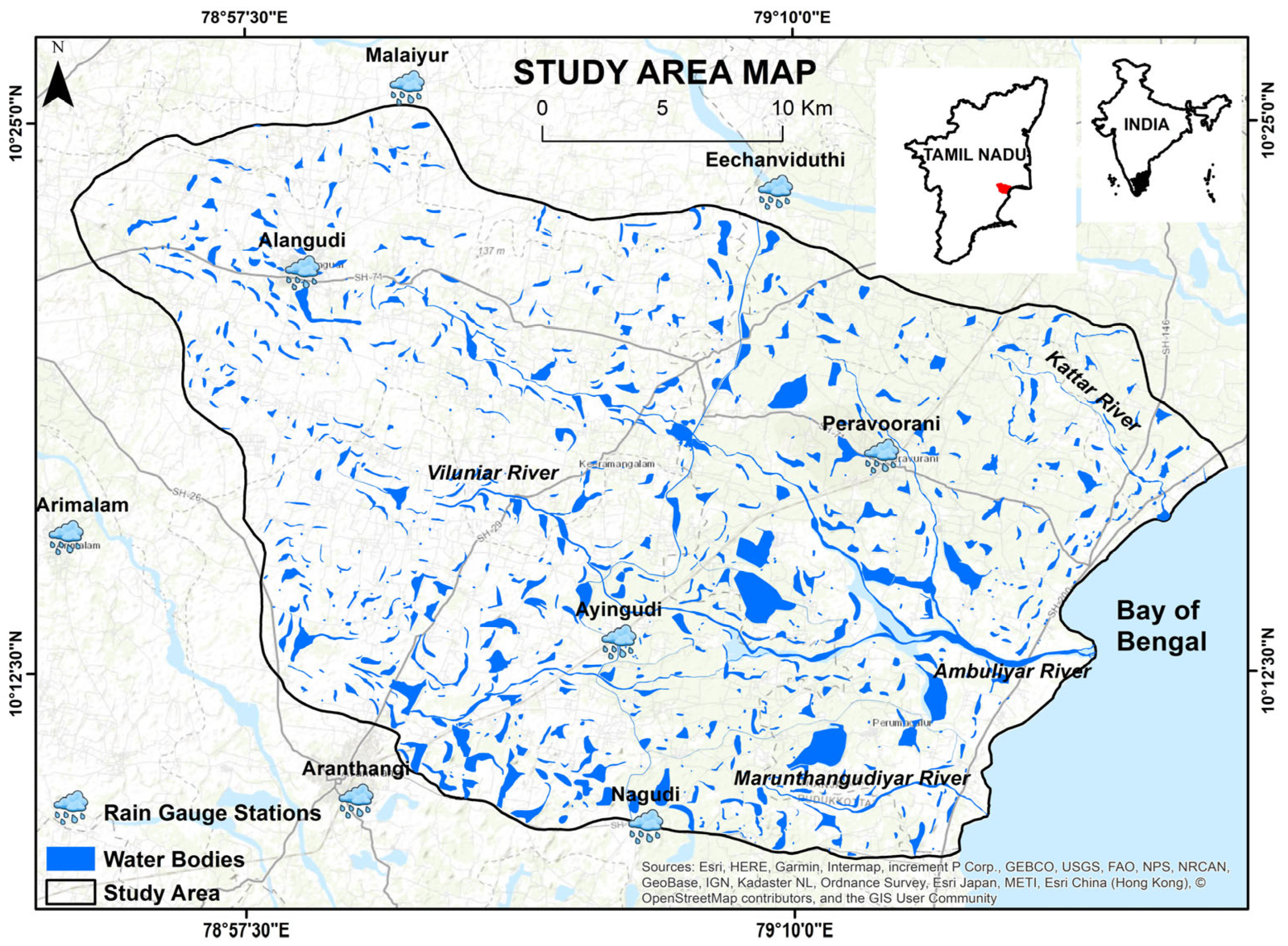
2.1. Study Area
2.2. Materials
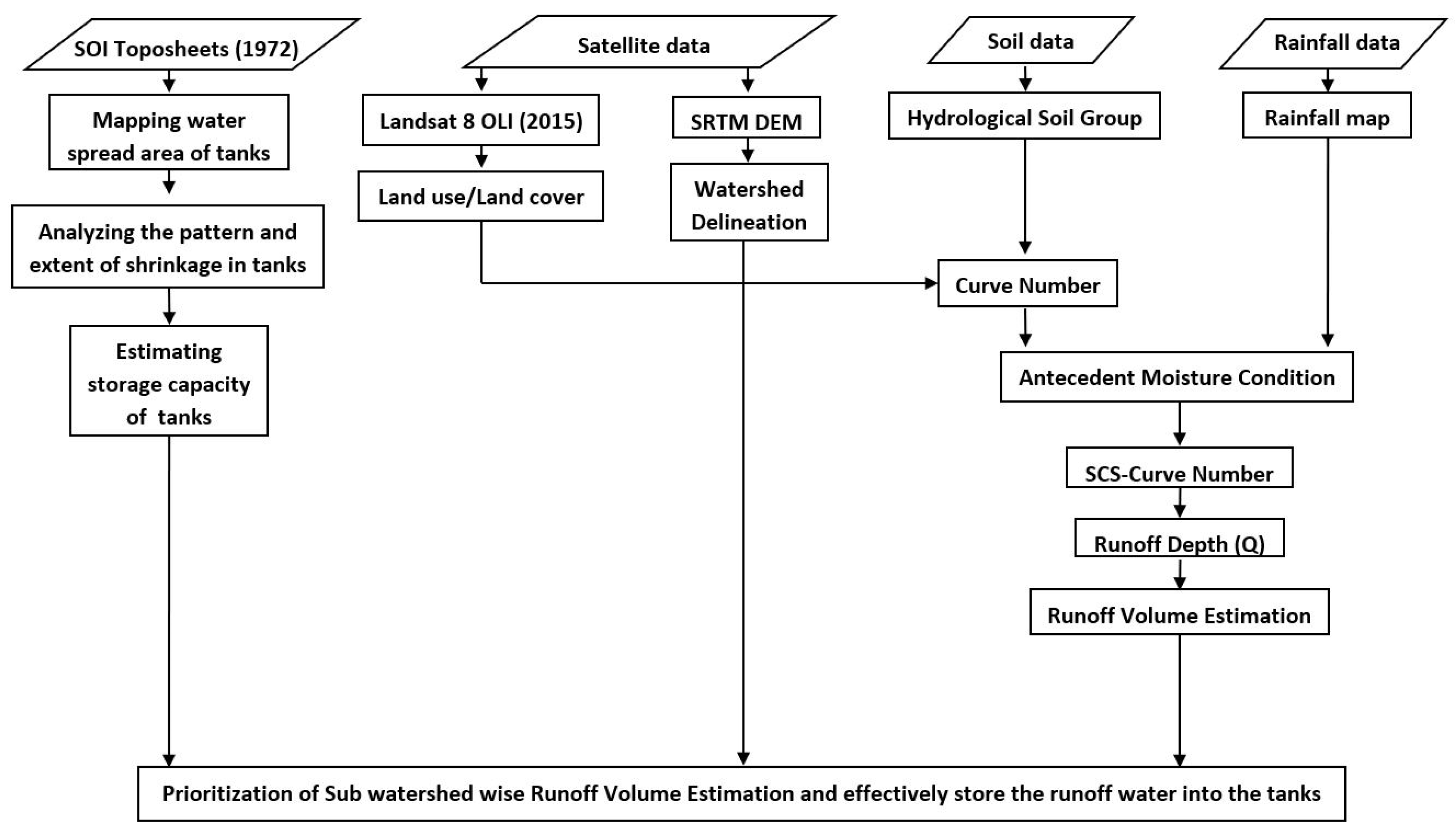
2.3. Methods
2.4. S.C.S.–C.N. Model
2.4.1. Weighted Curve Number
2.4.2. Calculation of Run-Off Depth (Q)
- Q = direct flow volume represented in depth (mm)
- P = rainfall (mm)
- S = potential maximum soil retention
3. Results and Discussion
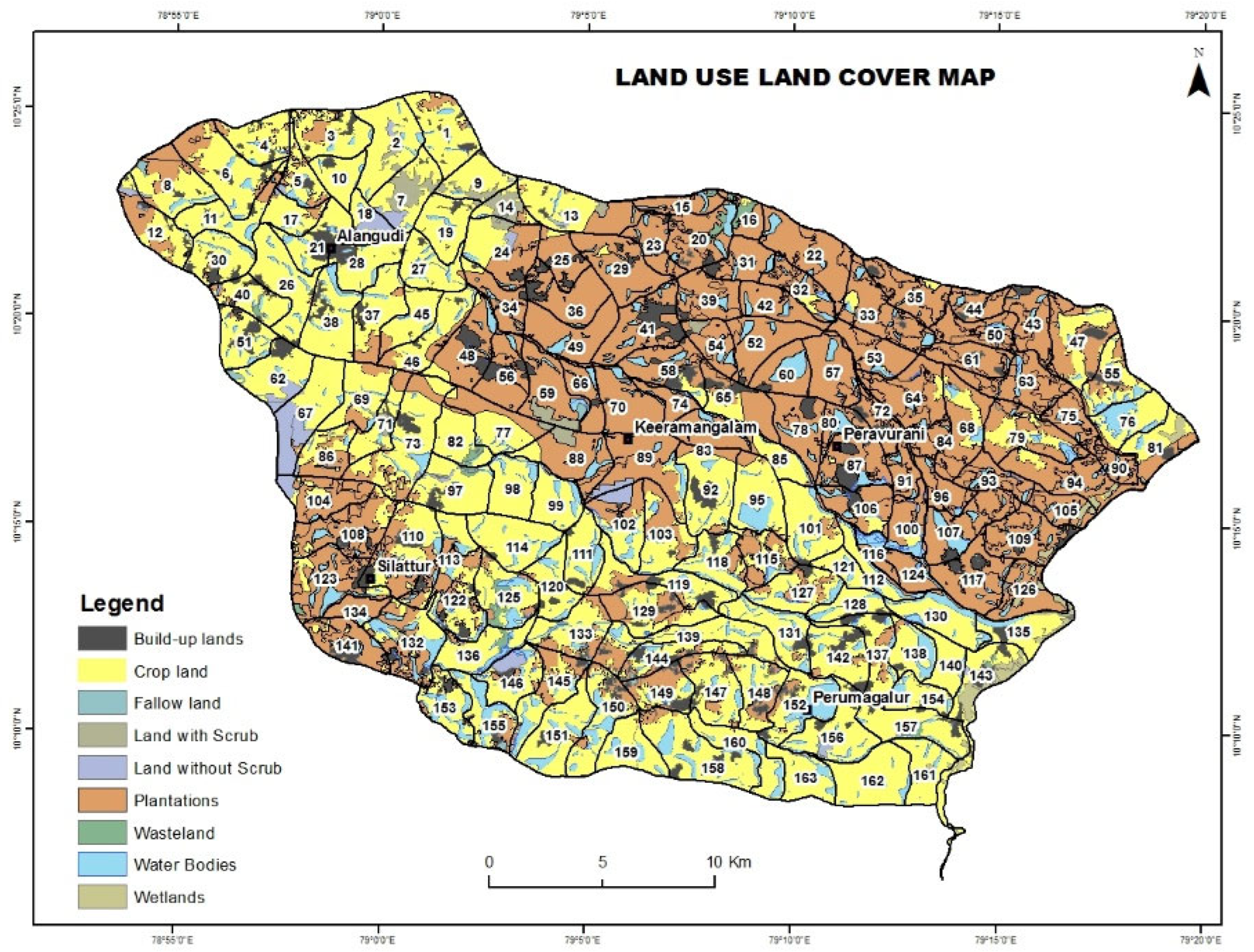
3.1. Land Use and Land Cover
3.2. Hydrological Soil Group Map
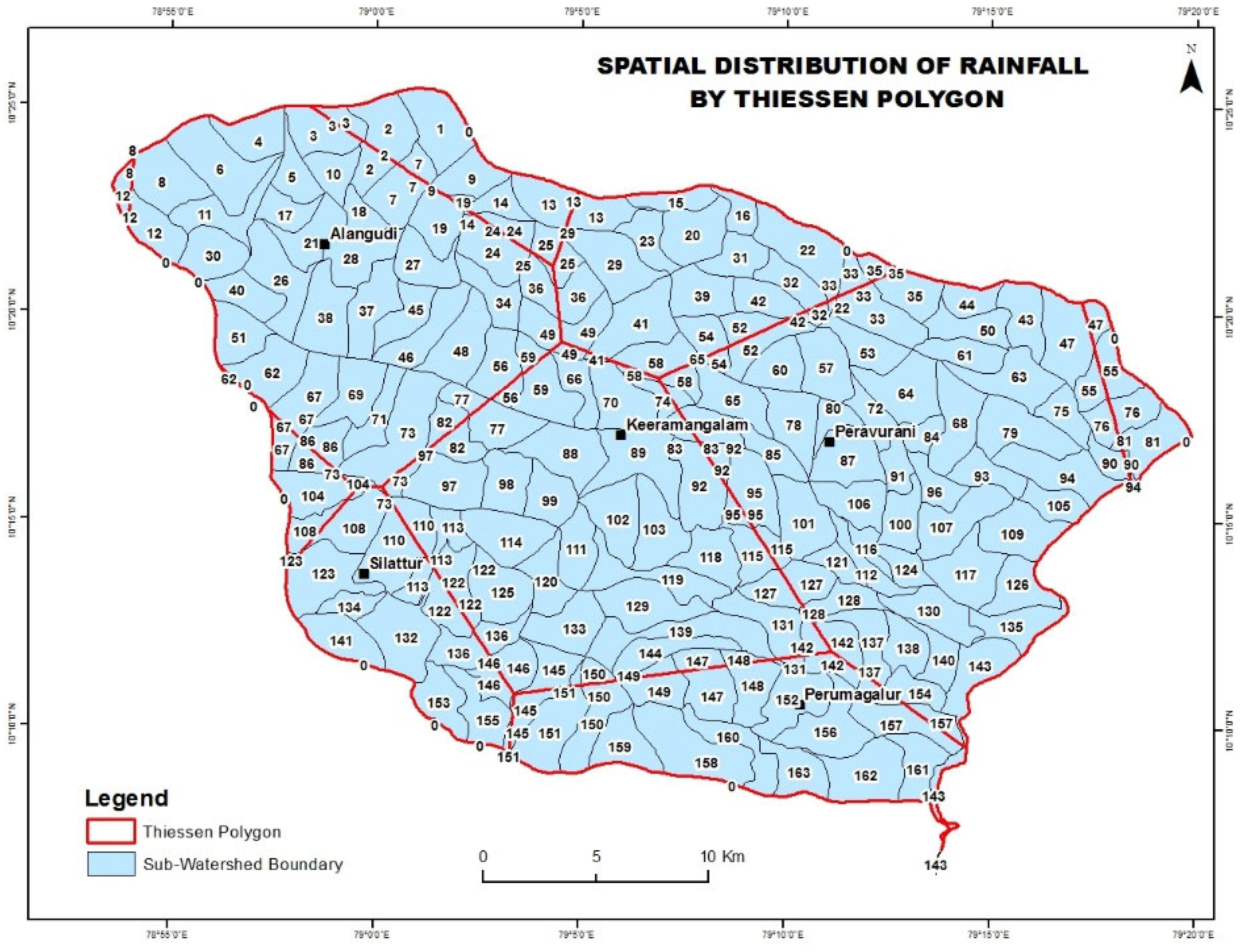
3.3. Rainfall
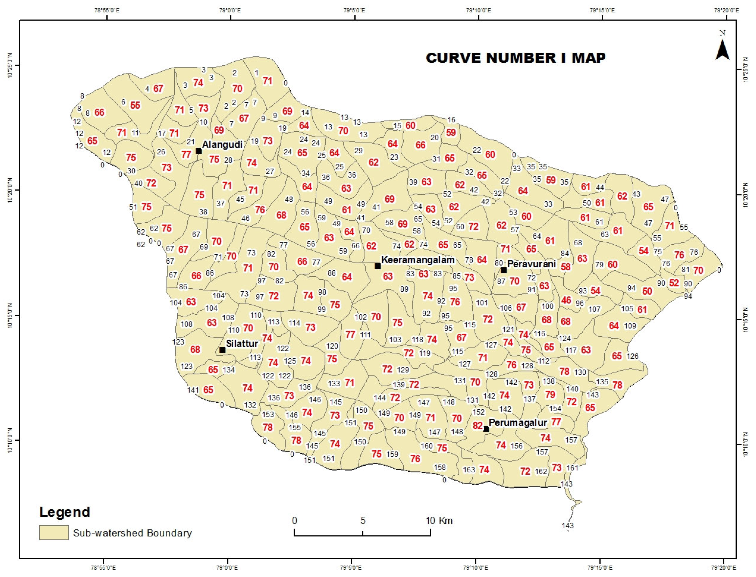
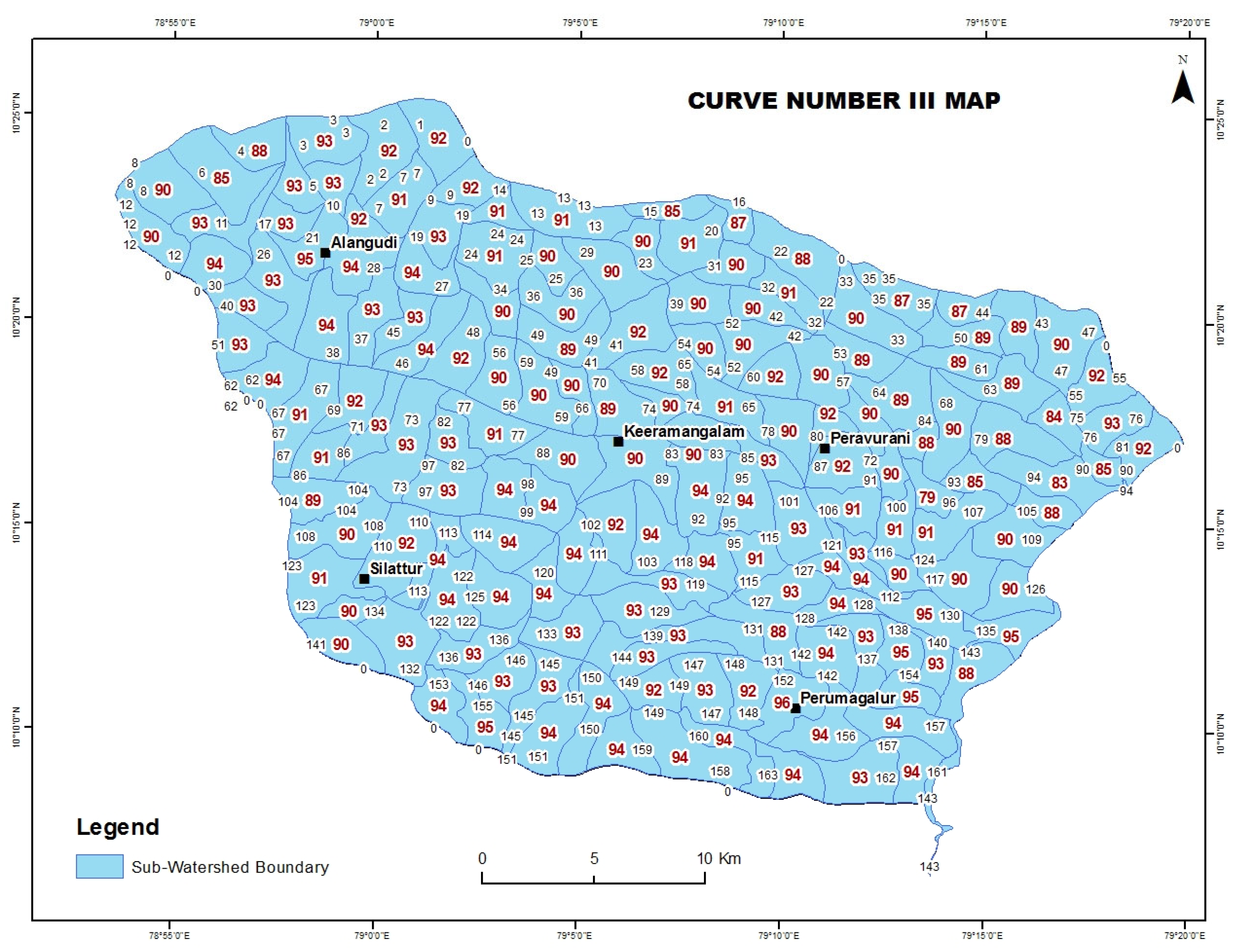
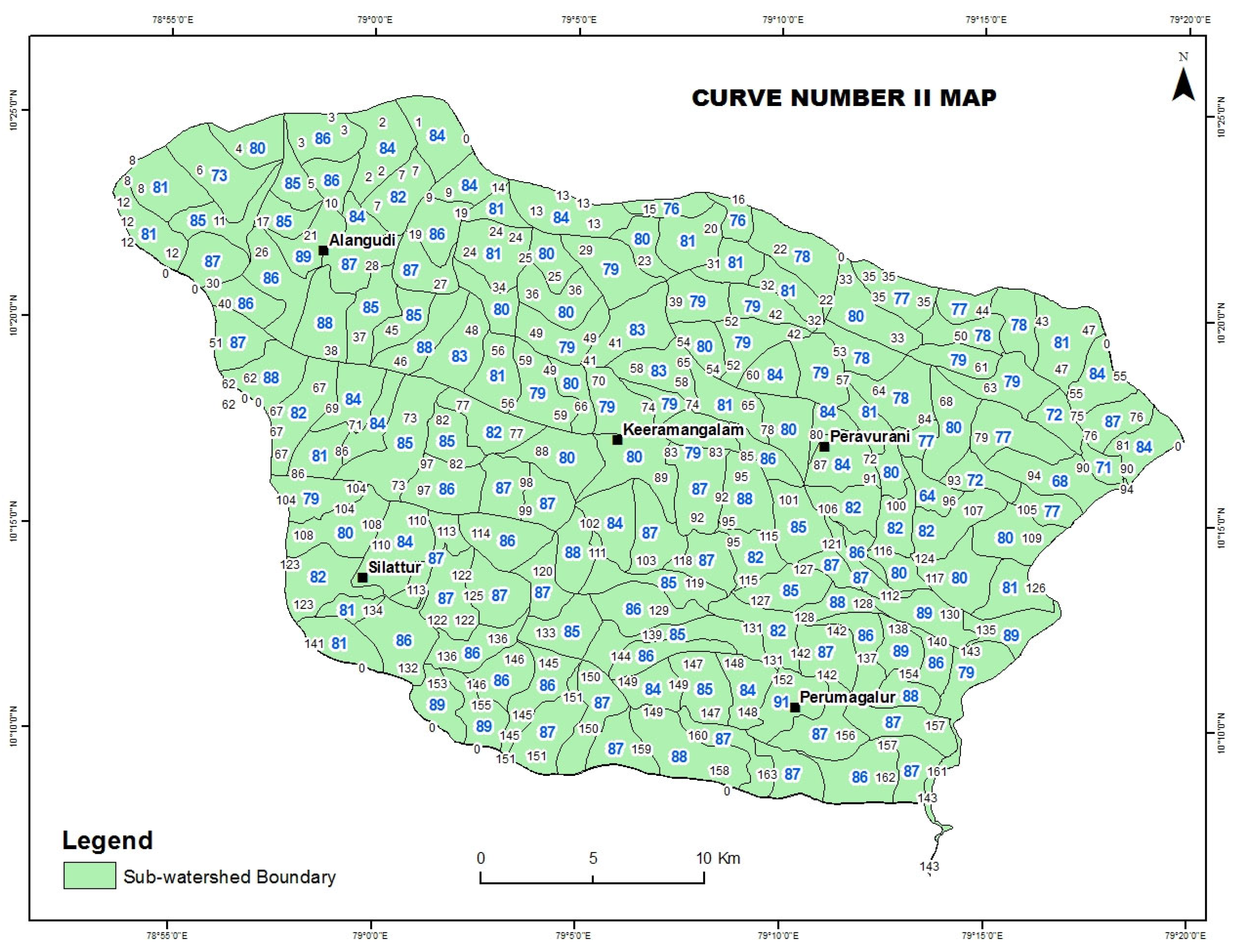
3.4. Derivation of Weighted Curve Number
3.5. Calculation of Run-Off Volume
4. Discussion
5. Conclusions
Supplementary Materials
Author Contributions
Funding
Data Availability Statement
Acknowledgments
Conflicts of Interest
References
- Ramarao, M.V.S.; Sanjay, J.; Krishnan, R.; Mujumdar, M.; Bazaz, A.; Revi, A. On Observed Aridity Changes over the Semiarid Regions of India in a Warming Climate. Theor. Appl. Climatol. 2019, 136, 693–702. [Google Scholar] [CrossRef]
- Chowdhury, K.; Behera, B. Is Declining Groundwater Levels Linked with the Discontinuity of Traditional Water Harvesting Systems (tank Irrigation)? Empirical Evidence from West Bengal, India. Groundw. Sustain. Dev. 2018, 7, 185–194. [Google Scholar] [CrossRef]
- Goyal, M.R.; Panigrahi, P. Sustainable Micro Irrigation Design Systems for Agricultural Crops: Methods and Practices; CRC Press: Boca Raton, FL, USA, 2015; ISBN 9781771882750. [Google Scholar]
- Sakthivadivel, R.; Thiruvengadachari, S.; Bastiaanssen, U.; Molden, D. Performance Evaluation of the Bhakra Irrigation System, India, Using Remote Sensing and GIS Techniques; IWMI: Colombo, Sri Lanka, 1999; ISBN 9789290903758. [Google Scholar]
- Angelakιs, A.N.; Zaccaria, D.; Krasilnikoff, J.; Salgot, M.; Bazza, M.; Roccaro, P.; Jimenez, B.; Kumar, A.; Yinghua, W.; Baba, A.; et al. Irrigation of World Agricultural Lands: Evolution through the Millennia. Water 2020, 12, 1285. [Google Scholar] [CrossRef]
- Pant, N.; Verma, R.K. Tanks in Eastern India: A Study in Exploration; IWMI: Colombo, Sri Lanka, 2010; ISBN 9789290907312. [Google Scholar]
- Barah, B.C. Traditional Water Harvesting Systems: An Ecological Economic Appraisal; New Age International: New York, NY, USA, 1996. [Google Scholar]
- Asian Development Bank. Irrigation Management Transfer: Strategies and Best Practices; Sage Publications: Thousand Oaks, CA, USA, 2008. [Google Scholar]
- Vaidyanathan, A. Water Management and Agriculture in the Palar and the Parambikulam Aliyar Systems in Tamil Nadu; Madras Institute of Development Studies: Tamil Nadu, India, 2004. [Google Scholar]
- Neelakantan, T.R.; Suribabu, C.R.; Selvakumar, R. Opportunity to Restore Irrigation Tanks in the Cauvery Delta by Mining and Deepening. Environ. Dev. Sustain. 2017, 19, 1463–1472. [Google Scholar] [CrossRef]
- Palanisami, K.; Meinzen-Dick, R.; Giordano, M. Climate Change and Water Supplies: Options for Sustaining Tank Irrigation Potential in India; Economic & Political Weekly: Mumbai, India, 2010. [Google Scholar]
- Singh, R.; Akuraju, V.; Anantha, K.H.; Garg, K.K.; Barron, J.; Whitbread, A.M.; Dev, I.; Dixit, S. Traditional Rainwater Management (Haveli cultivation) for Building System Level Resilience in a Fragile Ecosystem of Bundelkhand Region, Central India. Front. Sustain. Food Syst. 2022, 6, 826722. [Google Scholar] [CrossRef]
- De Silva, D.A.; Anderson, E.A.; Kim, J.; Ting Lee, M.-L.; Thoma, M.E. The Association Between Prenatal Food Insecurity and Breastfeeding Initiation and Exclusive Breastfeeding Duration: A Longitudinal Study Using Oregon PRAMS and PRAMS-2, 2008–2015. Breastfeed. Med. 2024, 19, 368–377. [Google Scholar] [CrossRef]
- Gajbhiye, S.; Mishra, S.K.; Pandey, A. Simplified Sediment Yield Index Model Incorporating Parameter Curve Number. Arab. J. Geosci. 2015, 8, 1993–2004. [Google Scholar] [CrossRef]
- Meshram, S.G.; Sharma, S.K. Prioritization of Watershed through Morphometric Parameters: A PCA-Based Approach. Appl. Water Sci. 2017, 7, 1505–1519. [Google Scholar] [CrossRef]
- Santra, A.; Mitra, S.S. Remote Sensing Techniques and GIS Applications in Earth and Environmental Studies; IGI Global: Hershey, PA, USA, 2016; ISBN 9781522518150. [Google Scholar]
- International Association of Hydrological Sciences. Scientific Assembly Remote Sensing and Geographic Information Systems for Design and Operation of Water Resources Systems; International Association of Hydrological Sciences: Wallingford, UK, 1997; ISBN 9781901502152. [Google Scholar]
- Pachpute, J.S.; Tumbo, S.D.; Sally, H.; Mul, M.L. Sustainability of Rainwater Harvesting Systems in Rural Catchment of Sub-Saharan Africa. Water Resour. Manag. 2009, 23, 2815–2839. [Google Scholar] [CrossRef]
- Khaleghi, M.R. The Influence of Deforestation and Anthropogenic Activities on Run-off Generation. J. Forensic Sci. 2017, 63, 245–253. [Google Scholar]
- Tripathi, A.; Attri, L.; Tiwari, R.K. Spaceborne C-Band SAR Remote Sensing-Based Flood Mapping and Run-off Estimation for 2019 Flood Scenario in Rupnagar, Punjab, India. Environ. Monit. Assess. 2021, 193, 110. [Google Scholar] [CrossRef] [PubMed]
- Mishra, S.K.; Singh, V.P. Soil Conservation Service Curve Number (SCS-CN) Methodology; Springer Science & Business Media: Berlin/Heidelberg, Germany, 2013; ISBN 9789401701471. [Google Scholar]
- Nasir, N.; Selvakumar, R. Influence of Land Use Changes on Spatial Erosion Pattern, a Time Series Analysis Using RUSLE and GIS: The Cases of Ambuliyar Sub-Basin, India. Acta Geophys. 2018, 66, 1121–1130. [Google Scholar] [CrossRef]
- Nasir, N.; Selvakumar, R. Estimating the Loss of Water Spread Area in Tanks Using Remote Sensing and GIS Techniques in Ambuliyar Sub-Basin, Tamilnadu. In Lecture Notes in Civil Engineering; Springer Science & Business Media: Berlin/Heidelberg, Germany, 2021. [Google Scholar]
- Satheeshkumar, S.; Venkateswaran, S.; Kannan, R. Rainfall–run-off Estimation Using SCS–CN and GIS Approach in the Pappiredipatti Watershed of the Vaniyar Sub Basin, South India. Model. Earth Syst. Environ. 2017, 3, 1–8. [Google Scholar] [CrossRef]
- El-Bagoury, H.; Gad, A. Integrated Hydrological Modeling for Watershed Analysis, Flood Prediction, and Mitigation Using Meteorological and Morphometric Data, SCS-CN, HEC-HMS/RAS, and QGIS. Water 2024, 16, 356. [Google Scholar] [CrossRef]
- ASCE/EWRI Curve Number Hydrology Task Committee; Hawkins, R.H. Curve Number Hydrology: State of the Practice; Amer Society of Civil Engineers: Reston, VA, USA, 2009; ISBN 9780784410042. [Google Scholar]
- Beven, K.J. Rainfall-Runoff Modelling: The Primer; John Wiley & Sons: Hoboken, NJ, USA, 2012; ISBN 9780470714591. [Google Scholar]
- Abraham, S.; Huynh, C.; Vu, H. Classification of Soils into Hydrologic Groups Using Machine Learning. Brown Univ. Dig. Addict. Theory Appl. 2019, 5, 2. [Google Scholar] [CrossRef]
- Rani, S. Climate, Land-Use Change and Hydrology of the Beas River Basin, Western Himalayas; Springer Nature: Berlin/Heidelberg, Germany, 2023; ISBN 9783031295256. [Google Scholar]
- Di Gregorio, A.; Food and Agriculture Organization of the United Nations. Land Cover Classification System: Classification Concepts and User Manual: LCCS; Food & Agriculture Org.: Rome, Italy, 2005; ISBN 9789251053270. [Google Scholar]
- National Research Council; Division on Earth and Life Studies; Board on Earth Sciences and Resources; Geographical Sciences Committee; Committee on Needs and Research Requirements for Land Change Modeling. Advancing Land Change Modeling: Opportunities and Research Requirements; National Academies Press: Washington, DC, USA, 2014; ISBN 9780309288361. [Google Scholar]
- Moon, G.W.; Ajmal, M.; Ahn, J.H.; Kim, T.W. Investigating practical alternatives to the NRCS-CN method for direct run-off estimation using slope-adjusted curve numbers. KSCE J. Civ. Eng. 2016, 20, 3022–3030. [Google Scholar] [CrossRef]
- Matomela, N.; Tianxin, L.; Morahanye, L.; Bishoge, O.K.; Ikhumhen, H.O. Rainfall-runoff estimation of Bojiang lake watershed using SCS-CN model coupled with GIS for watershed management. J. Appl. Adv. Res. 2019, 4, 16–24. [Google Scholar] [CrossRef]
- Nasiri, V.; Deljouei, A.; Moradi, F.; Sadeghi, S.M.M.; Borz, S.A. Land Use and Land Cover Mapping Using Sentinel-2, Landsat-8 Satellite Images, and Google Earth Engine: A Comparison of Two Composition Methods. Remote Sens. 2022, 14, 1977. [Google Scholar] [CrossRef]
- Saralioglu, E.; Vatandaslar, C. Land Use/land Cover Classification with Landsat-8 and Landsat-9 Satellite Images: A Comparative Analysis between Forest- and Agriculture-Dominated Landscapes Using Different Machine Learning Methods. Acta Geod. Geophys. 2022, 57, 695–716. [Google Scholar] [CrossRef]
- Kumar, A.; Kanga, S.; Taloor, A.K.; Singh, S.K.; Đurin, B. Surface Run-off Estimation of Sind River Basin Using Integrated SCS-CN and GIS Techniques. HydroResearch 2021, 4, 61–74. [Google Scholar] [CrossRef]
- Available online: https://www.plantarchives.org/SPL%20ISSUE%2020-2/178__1156-1160_.pdf (accessed on 27 March 2024).
- Masruroh, H.; Soemarno, S.; Kurniawan, S.; Leksono, A.S. A Spatial Model of Landslides with A Micro-Topography and Vegetation Approach for Sustainable Land Management in the Volcanic Area. Sustain. Sci. Pract. Policy 2023, 15, 3043. [Google Scholar] [CrossRef]
- Rizeei, H.M.; Pradhan, B.; Saharkhiz, M.A. Surface Run-off Prediction Regarding LULC and Climate Dynamics Using Coupled LTM, Optimised ARIMA, and GIS-Based SCS-CN Models in Tropical Region. Arab. J. Geosci. 2018, 11, 1–16. [Google Scholar] [CrossRef]
- Guzha, A.C.; Nobrega, R.L.B.; Kovacs, K.; Rebola-Lichtenberg, J.; Amorim, R.S.S.; Gerold, G. Characterizing Rainfall-Run-off Signatures from Micro-Catchments with Contrasting Land Cover Characteristics in Southern Amazonia. Hydrol. Process. 2015, 29, 508–521. [Google Scholar] [CrossRef]
- Puttaswamy, N.K.; Kulkarni, G.N. Rehabilitation of Tank Systems and Its Impact on Farm Economy: An Empirical Analysis in Haveri District of Karnataka, India; LAP Lambert Academic Publishing: Saarbrucken, Germany, 2015; ISBN 9783659764103. [Google Scholar]
- Karthikeyan, C.; Suresh Kumar, D.; Palanisamy, K. Sustainable Management of Tank System in South India; LAP Lambert Academic Publishing: Saarbrucken, Germany, 2012; ISBN 9783659208997. [Google Scholar]
- Amarnath, J.S.; Karthik Raja, P. Examined the economic benefits of tank rehabilitation in Madurai District, Tamil Nadu. Agric. Econ. Res. Rev. 2006, 19(1), 187–194. [Google Scholar]
- Anuradha, B.; Packialakshmi, S.; Sanjay, N.; Vivekananthan, V. An Analytical Study for Assessing Water Productivity in Pre- and Post-Rehabilitation Period of Rural Tank System. Adv. Civ. Eng. 2022, 2022, 1119931. [Google Scholar] [CrossRef]
- Deivalatha, A.; Senthilkumaran, P.; Ambujam, N.K. Impact of desilting of irrigation tanks on productivity of crop yield and profitability of farm income. Acad. J. 2014, 9, 1833–1840. [Google Scholar] [CrossRef]


| S. No | Used Data | Scale/Data Resolution | Year/Range | Source |
|---|---|---|---|---|
| 1 | DEM-SRTM (1 Arc sec) | 30 m | 23 September 2014 | U.S.G.S. (https://earthexplorer.usgs.gov/ accessed on 1 May 2024) |
| 2 | Landsat-8 | 30 m | 2 January 2023 | U.S.G.S. (https://earthexplorer.usgs.gov/ accessed on 1 May 2024) |
| 3 | Soil Data | 1:50,000 | Tamil Nadu Agriculture Department | |
| 4 | Rainfall Data | 1975 to 2021 | Indian Meteorological Department | |
| 5 | Topographic Sheets | 1:50,000 | Survey of India |
| S. No | Rain Gauge Stations | Latitude | Longitude |
|---|---|---|---|
| 1 | Nagudi | 10.15 | 79.11 |
| 2 | Ayingudi | 10.22 | 79.1 |
| 3 | Aranthangi | 10.16 | 79 |
| 4 | Arimalam | 10.26 | 78.89 |
| 5 | Pudukottai | 10.38 | 78.82 |
| 6 | Perungalur | 10.49 | 78.93 |
| 7 | Malaiyur | 10.43 | 79.02 |
| 8 | Karambakudi | 10.46 | 79.13 |
| 9 | Alangudi | 10.36 | 78.98 |
| 10 | Adirampattinam | 10.34 | 79.39 |
| 11 | Eechanviduthi | 10.39 | 79.16 |
| 12 | Peravoorani | 10.29 | 79.2 |
| S.No | Properties | Group A | Group B | Group C | Group D |
|---|---|---|---|---|---|
| 1 | Infiltration rate | High | Moderate | Slow | Very slow |
| 2 | Texture | Coarse | Moderate | Fine | Very fine |
| 3 | Depth | Very deep | Moderately deep | Deep | Shallow |
| 4 | Water transmission | High | Moderate | Slow | Very slow |
| 5 | Run-off potential | Low | Moderate | High | Very high |
| S.No | Watershed Number | Rainfall Station |
|---|---|---|
| 1 | 70, 88, 89, 98, 99, 102, 103, 111, 114, 118, 119, 120, 125, 129, 131, 133, 139, 144, 147, 148, 149, 150 | Aayingudi |
| 2 | 2, 3, 4, 5, 6, 7, 8, 9, 10, 11, 12, 14, 17, 18, 19, 21, 24, 25, 26, 27, 28, 30, 34, 36, 37, 38, 40, 45, 46, 48, 49, 51, 56, 59, 66, 69, 71, 77, 82, 97 | Alangudi |
| 3 | 110, 113, 122, 132, 134, 136, 141, 145, 151, 153, 155 | Aranthangi |
| 4 | 62, 67, 73, 86, 104, 108, 123 | Arimalam |
| 5 | 13, 15, 16, 20, 23, 29, 31, 39, 41 | Eechanviduthi |
| 6 | 1 | Malaiyur |
| 7 | 152, 156, 158, 159, 160, 161, 162, 163 | Nagudi |
| 8 | 22, 32, 33, 35, 42, 43, 44, 47, 50, 52, 53, 54, 55, 57, 58, 60, 61, 63, 64, 65, 68, 72, 74, 75, 76, 78, 79, 80, 81, 83, 84, 85, 87, 90, 91, 92, 93, 94, 95, 96, 100, 101, 105, 106, 107, 109, 112, 115, 116, 117, 121, 124, 126, 127, 128, 130, 135, 137, 137, 140, 142, 142, 143, 154, 157 | Peravurani |
| S.No | LULC | HSG | Assigned CN-II | Area of Intersected LULC & HSG. | Intersected Area × CN-II |
|---|---|---|---|---|---|
| 1 | Build-up lands | Group-A | 89 | 0.75 | 66.67 |
| 2 | Build-up lands | Group-B | 92 | 0.82 | 75.14 |
| 3 | Build-up lands | Group-C | 94 | 42.54 | 3999.18 |
| 4 | Build-up lands | Group-D | 95 | 6.07 | 576.87 |
| 5 | Cropland | Group-A | 67 | 9.63 | 645.34 |
| 6 | Cropland | Group-B | 78 | 0.78 | 60.91 |
| 7 | Cropland | Group-C | 85 | 341.68 | 29,043.19 |
| 8 | Cropland | Group-D | 89 | 31.68 | 2819.9 |
| 9 | Fallow land | Group-C | 74 | 1.35 | 99.89 |
| 10 | Land with Scrub | Group-B | 68 | 0.09 | 6.43 |
| 11 | Land with Scrub | Group-C | 79 | 8.84 | 698.31 |
| 12 | Land with Scrub | Group-D | 84 | 0.28 | 23.66 |
| 13 | Land without Scrub | Group-B | 69 | 0.05 | 3.71 |
| 14 | Land without Scrub | Group-C | 79 | 12.41 | 980.77 |
| 15 | Land without Scrub | Group-D | 84 | 0.29 | 24.26 |
| 16 | Plantations | Group-A | 45 | 5.22 | 234.81 |
| 17 | Plantations | Group-B | 66 | 10.48 | 691.92 |
| 18 | Plantations | Group-C | 77 | 346.27 | 26,662.78 |
| 19 | Plantations | Group-D | 83 | 13.01 | 1080.22 |
| 20 | Wasteland | Group-A | 49 | 0.06 | 3.11 |
| 21 | Wasteland | Group-B | 69 | 0.01 | 0.55 |
| 22 | Wasteland | Group-C | 79 | 4.43 | 350 |
| 23 | Wasteland | Group-D | 84 | 0.02 | 2.03 |
| 24 | Water Bodies | Group-A | 100 | 1.96 | 196.34 |
| 25 | Water Bodies | Group-B | 100 | 1.18 | 117.6 |
| 26 | Water Bodies | Group-C | 100 | 68.9 | 6890.22 |
| 27 | Water Bodies | Group-D | 100 | 14.15 | 1415.19 |
| 28 | Wetlands | Group-A | 91 | 1.19 | 108.7 |
| 29 | Wetlands | Group-B | 95 | 0 | 0.08 |
| 30 | Wetlands | Group-C | 96 | 5.78 | 554.49 |
| 31 | Wetlands | Group-D | 98 | 0.33 | 32.67 |
| Total | 930.3 | 77,464.95 | |||
| (Intersected area × CN-II)/Area of Sub Watershed = Weighted CN-II 77,464.95/930.30 = 83.27 | |||||
Disclaimer/Publisher’s Note: The statements, opinions and data contained in all publications are solely those of the individual author(s) and contributor(s) and not of MDPI and/or the editor(s). MDPI and/or the editor(s) disclaim responsibility for any injury to people or property resulting from any ideas, methods, instructions or products referred to in the content. |
© 2024 by the authors. Licensee MDPI, Basel, Switzerland. This article is an open access article distributed under the terms and conditions of the Creative Commons Attribution (CC BY) license (https://creativecommons.org/licenses/by/4.0/).
Share and Cite
Nagoor Pitchai, N.; Magalingam, S.; Rajasekaran, S.K.D.; Radhakrishnan, S. Cost-Benefit Analysis of Minor Irrigation Tank Rehabilitation Using Run-Off and Storage Capacity: A Case Study from Ambuliyar Sub-Basin, Tamil Nadu, India. GeoHazards 2024, 5, 441-456. https://doi.org/10.3390/geohazards5020023
Nagoor Pitchai N, Magalingam S, Rajasekaran SKD, Radhakrishnan S. Cost-Benefit Analysis of Minor Irrigation Tank Rehabilitation Using Run-Off and Storage Capacity: A Case Study from Ambuliyar Sub-Basin, Tamil Nadu, India. GeoHazards. 2024; 5(2):441-456. https://doi.org/10.3390/geohazards5020023
Chicago/Turabian StyleNagoor Pitchai, Nasir, Somasundharam Magalingam, Sakthi Kiran Duraisamy Rajasekaran, and Selvakumar Radhakrishnan. 2024. "Cost-Benefit Analysis of Minor Irrigation Tank Rehabilitation Using Run-Off and Storage Capacity: A Case Study from Ambuliyar Sub-Basin, Tamil Nadu, India" GeoHazards 5, no. 2: 441-456. https://doi.org/10.3390/geohazards5020023
APA StyleNagoor Pitchai, N., Magalingam, S., Rajasekaran, S. K. D., & Radhakrishnan, S. (2024). Cost-Benefit Analysis of Minor Irrigation Tank Rehabilitation Using Run-Off and Storage Capacity: A Case Study from Ambuliyar Sub-Basin, Tamil Nadu, India. GeoHazards, 5(2), 441-456. https://doi.org/10.3390/geohazards5020023