Abstract
The work detailed here is part of an international initiative on the evaluation of dam safety simulation software for internal erosion performance and best practices. The primary experiments involve simulating uncertainty in the failure events of two dams with two different models: DLBreach and WinDAM C. DLBreach is a physically-based dam/levee breach model developed by Wu. WinDAM C is also a physically based dam breach model capable of analyzing both dam overtopping and internal erosion. The dams selected for the analysis include a 1.3 m high dam tested in the lab and a larger 15.56 m high dam, which suffered a failure in the field. The findings from these experiments are extended with a further analysis on variance, sensitivity, and optimization. Finally, a regression model is trained using the results of these simulators as an inquiry into how well such a system can be captured using machine learning techniques. The results of these experiments, together with the results of the other members of the initiative, improve our understanding of the influences that users bring to using these tools.
1. Introduction
With some 41,000 large earthen dams across the world [1] and around 76,000 earthen dams of any size in the US alone [2], their impacts on the lives and livelihoods of many people is significant. The interest in accurately predicting dam breaches and the magnitude of the resulting breach hydrograph has increased during the past several decades. Some of the tools include equations based on data from historical events [3,4] and sediment transport models, such as those developed by Fread [5,6]. They have been used to accurately predict peak discharge and floodplain mapping, but they provide little information about the timing and physics of breach development or the impact of using different materials for the construction of the dam. More recently, research has focused on the response of embankment dams to both overtopping and internal erosion. Several physical model studies have been conducted. They involve a wide range of dams ranging from relatively small-scale embankments in the laboratory [7,8,9,10,11], to medium-scale embankments in large testing facilities [10,12,13,14], and large-scale embankments [15]. Because of this research, new computational models of breach erosion processes that more accurately reflect the observed behavior of cohesive soil embankments have been developed. WinDAM (Windows Dam Analysis Modules) is a desktop application that includes modules to analyze the overtopping and internal erosion of embankments, embankment breach development, and headcut erosion of earthen spillways. The individual modules and software as a whole are referred to as models. The models are tested and refined to improve model performance. On-site erodibility testing techniques, called a Jet test, have been developed to better quantify the erodibility of on-site soil materials [16,17,18]. These tests can be used to better quantify soil parameters on site.
The development and refinement of various models continues, as noted by several recent reviews and model evaluation efforts. ASCE/EWRI [19] provides a discussion of breach processes and tools available. The CEATI International Working Group on Embankment Dam Erosion and Breach Modeling [20] applied the HR Breach [21] and SIMBA [12] models to test cases, including laboratory tests and actual dam failures. HR Breach was developed by HR Wallingford. The CEATI report indicates that both models performed well on five of the seven test cases. Zhong et al. [22] discussed the NWS BREACH model [6], the HR Breach model, and the DLBreach model [23]. HR Wallingford has since developed EMBREA [24], a successor to HR Breach. Zhong et al. [25] conducted three large-scale physical model tests at the Nanjing Hydraulic Research Institute (NHRI) in China, and developed a new model to evaluate the overtopping breach processes of a cohesive dam. They compared their model with WinDAM and NWS Breach. Sensitivity analysis shows that all three models are sensitive to soil erodibility, but their proposed model and WinDAM are more sensitive than the National Weather Service (NWS) BREACH model.
Breach processes associated with overtopping and internal erosion are only imperfectly understood. To gain more of an understanding, an international group started an initiative to research how these tools differ in the hands of different modelers. An interesting phase of the initiative was to have modelers focus on the analysis of just two dams—one from the lab (P1) and one from an actual failure in the field (Big Bay). These results were then presented to the initiative and compared with those of the other participants.
The first dam, designated P1 and standing at roughly 1.3 m high, is well documented in the paper “Internal Erosion and Impact of Erosion Resistance” by Gregory Hanson, Ronald Tejral, Sherry Hunt, and Darrel Temple [10]. This work investigates the failure conditions surrounding internal breaches using medium-scale models. Given the controlled nature of these collapses, there is a wealth of data collected to accurately recreate them. This research was conducted at the United States Department of Agriculture—Agricultural Research Service’s Hydraulic Engineering Research Unit, which is responsible for much of the foundational work on earthen embankment safety and maintenance.
The other dam is the Big Bay dam in Mississippi where, in 2004, a piping failure led to the collapse of the dam and damage to the downstream area. The characteristics of this breach are estimated by Steven Yochum, Larry Goertz, and Phillip Jones in “Case Study of the Big Bay Dam Failure: Accuracy and Comparison of Breach Predictions” [26]. This description uses data gathered at the time of the breach and measurements taken afterwards. Given these circumstances, these measurements may be less accurate compared to those of the P1 dam in its controlled environment. However, natural variance will also contribute greatly.
The two models that this paper reports on are DLBreach and WinDAM C. DLBreach, developed by Dr. Weiming Wu of Clarkson University [23,27], is a command-line application designed to analyze earthen dam and levee breaches. WinDAM C, developed jointly by the USDA and Kansas State University [14], is a GUI desktop application that includes several hydrologic routing functions, including the analysis of overtopping and internal erosion breaches. Aside from front-end differences, these simulators also differ in the way in which they represent their domain data and carry out their simulations.
To automate the processing of multiple simulation jobs, the Dakota suite developed by Sandia National Laboratories [28] is linked to these simulators via a process outlined by Mitchell Neilsen and Chendi Cao in “Coupled Dam Safety Analysis using BREACH and WinDAM” [29]. New parsers have been developed to process the input and output for DLBreach.
This article presents an uncertainty analysis of DLBreach and WinDAM C for a large-scale real-world dam (Big Bay) and a medium-scale model dam (P1). This analysis includes comparing the output distributions from these simulators to one another and to real-world observations. Additionally, the individual results are ranked based on how well they model the observed conditions to investigate the per-run relationship between inputs and outputs. This research is then extended with a variance analysis to determine the significance of the influence each parameter has on the models. Finally, parameter optimization is used as a more rigorous approach to evaluating the performance of individual runs. Several methods are employed, including traditional techniques and machine learning. While the traditional approach is used as the basis for evaluation, the results from the machine learning approach are included to demonstrate its suitability in the field of earthen embankment simulations given proper care.
2. Materials and Methods
2.1. Dakota
Dakota can be used for a number of simulation experiments, including uncertainty analysis, parameter optimization, and sensitivity analysis. With the method outlined by Neilsen and Cao, the analysis driver for a Dakota study can be used to bi-directionally link Dakota to the models. The driver is a script outlining the steps in a study. Processing before and after the model execution is achieved by adding custom scripts to the analysis driver. This additional processing includes conversions between units and deriving secondary metrics from the outputs of the models. When the models are run, Dakota populates a template file with the appropriate values to create a configuration file for use by the models. The results of each run are then aggregated into a single output file.
2.2. Parameters
To describe the dams and their collapse events, three categories of parameters are presented. One category is dimensional data, such as the length, width, height, and slope ratios of the dams, as well as the initial dimensions of the breach. Another is soil properties, such as particle diameter, cohesion, erodibility, and critical shear stress. Finally, there is the hydrologic data category, such as reservoir volume profiles and inlet/outlet flow over time. A list of the parameters addressed in this study is presented in Table 1, though additional parameters were provided to modelers. The parameters are arranged into the three categories and ordered within each by how many of the models use that parameter.

Table 1.
Ranges and averages for dam parameter values.
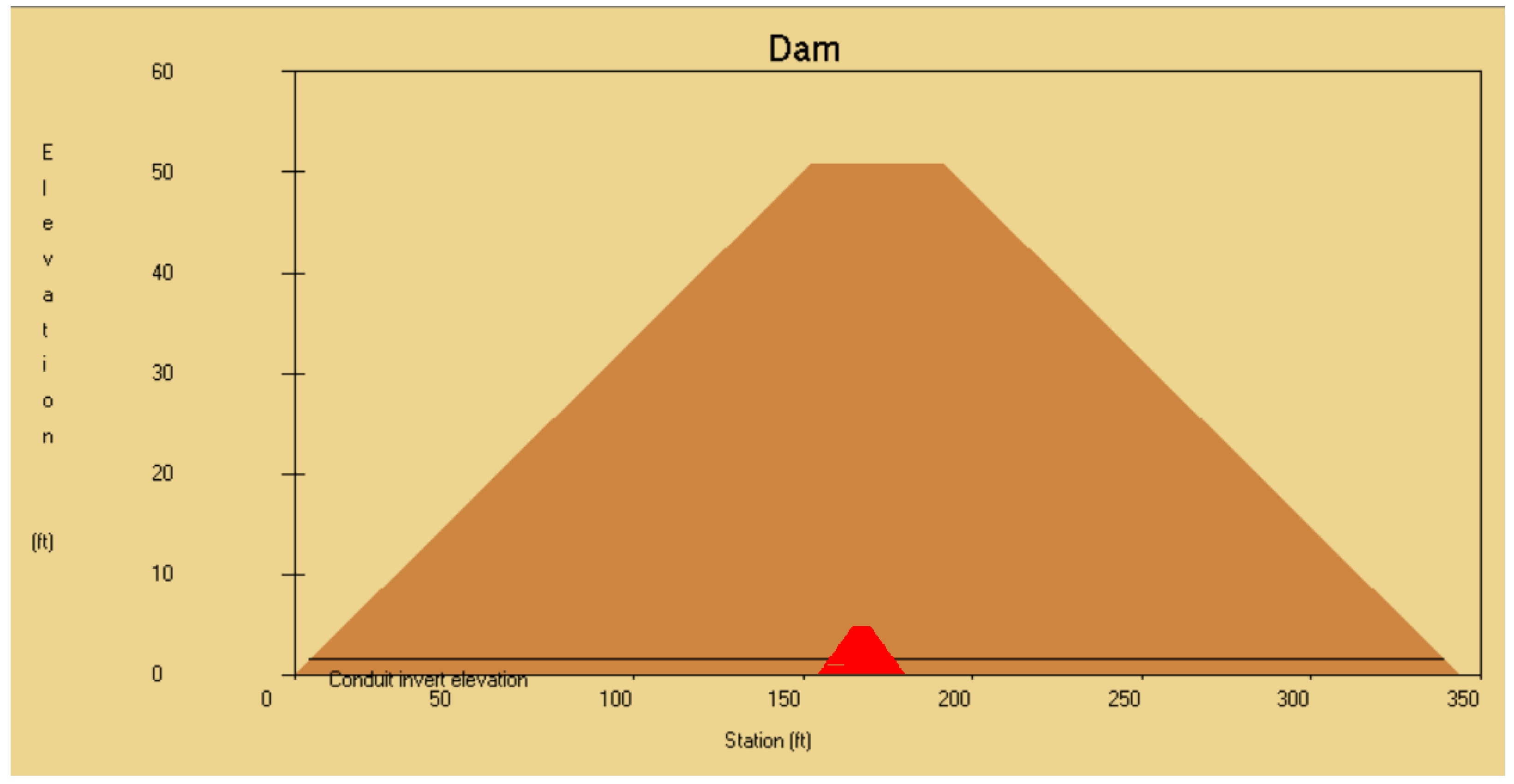
Due, in part, to natural variance and potential imprecision in measuring, the values of these parameters are presented as ranges. Alongside these ranges is an estimate of the average value, which is used as the mode of a triangular distribution. These ranges and defaults are estimates based on published work [13,17]. To better visualize the difference in dimensions between the two dams, Figure 1 shows a comparison of their side profiles.
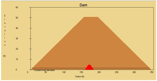
Figure 1.
Comparison of the side profiles of the Big Bay (brown) and P1 (red) dams.
2.3. Uncertainty Analysis
Using Dakota’s uncertainty analysis option, the experiment can be defined through a set of input parameters and output metrics. Input parameters are sampled as probability distributions determined through values specific to the type of distribution being used. For this experiment, the parameters were assumed to follow a triangular distribution with lower and upper limits as well as a mode. The output metrics of interest and their observed measurements are listed in Table 2. For the full study, additional metrics pertaining to the collapse of the breach roof were also tracked, but are not be included here. One goal of this experiment is to determine the distributions of these output metrics as output by the models.

Table 2.
Observed measurements of metrics.
In addition to the inputs and outputs, another important aspect is the number of simulations to run. Enough samples must be obtained such that the apparent distributions of the metrics are relatively stable. Stability, in this case, means that the numeric characteristics of these distributions are affected little by further simulations. For this study, the difference between 100 runs and 500 runs showed little improvement in the quality of the distributions; therefore, batches of 100 runs were used for convenience.
2.4. Variance Analysis
The uncertainty results are evaluated in R for significance using a standard analysis of variance. Although the whole table was generated in this way, only the p-value was included as the primary focus. The relationship between inputs and each output metric was formulated as a linear equation with no covariates. This formulation has limitations, which will be discussed later.
2.5. Optimization Analysis
The relationships examined in the uncertainty analysis are supplemented by a parameter optimization study. Four methods of optimization are used here, each with their own benefits and drawbacks. Three methods present practical approaches for their particular application, while one represents the kind of naïve approach that researchers might investigate.
The guidelines of the initiative provide a method for ranking results based on performance functions with the aim of investigating the relationship between inputs and outputs for any given individual run. These functions use the sum of the squared natural logarithms of the proportion of simulation values to estimated values. For this article, we focused on one of these functions, which uses the metrics for peak flow rate, time to peak flow, and maximum breach width from Table 2. Features of this kind of formulation that benefit the analysis include making exact matches equal to zero, making all outputs non-negative, and adjusting the ranges of possible outputs below and above the target value to be equally weighted. Thus, performance values closer to zero are better. In addition to the performance function, the average percent error of all output metrics was used for the sake of comparison.
To determine the limits of model performance in a more rigorous manner, another method was employed. Dakota provides a wealth of parameter optimization approaches, including several gradient-based and derivative-free methods. For this study, the asynchronous pattern search method was used based on the nature of the data. This is a kind of local search, but starting with a rough estimate can improve this search by reducing the search time and aid in preventing the search from becoming stuck in a local optimum. The configuration for this study has a similar format to the uncertainty experiment, but requires an objective function to optimize on. To achieve this, the performance function from earlier and the average percent error were added as two options for optimization.
The last two methods utilize machine learning by training regression models to emulate the results of the original models without having to carry out a full simulation. The data for this could be drawn from the uncertainty analysis, but instead, new simulations were run with an even spacing between parameter values. This allowed for the full breadth coverage of the parameter space at varying resolutions depending on the number of divisions. As the resolution becomes finer, a better approximation of the underlying function is presented. Due to the number of parameters, even three values per input can lead to tens of thousands of simulations. Therefore, three is the upper limit of divisions for this study.
Using the scikit-learn library for Python, an XGBoost model was trained with cross-validation. A ratio of 4:1 training vs testing material was used. As will be seen, a model of sufficient quality can be attained in a relatively short training time.
The first method demonstrates the naïve approach that instead trains a reverse model where the metrics are the input and parameter values are the output. This method aims to create a simple function to directly obtain the desired values. However, the issue with this approach is the assumptions that are required for it to work, as will be discussed.
A more standard approach addresses these issues by using the trained model as a surrogate in a typical optimization search. A dual-annealing implementation provided by the ScyPi library was then used for the actual search.
3. Results
3.1. Uncertainty
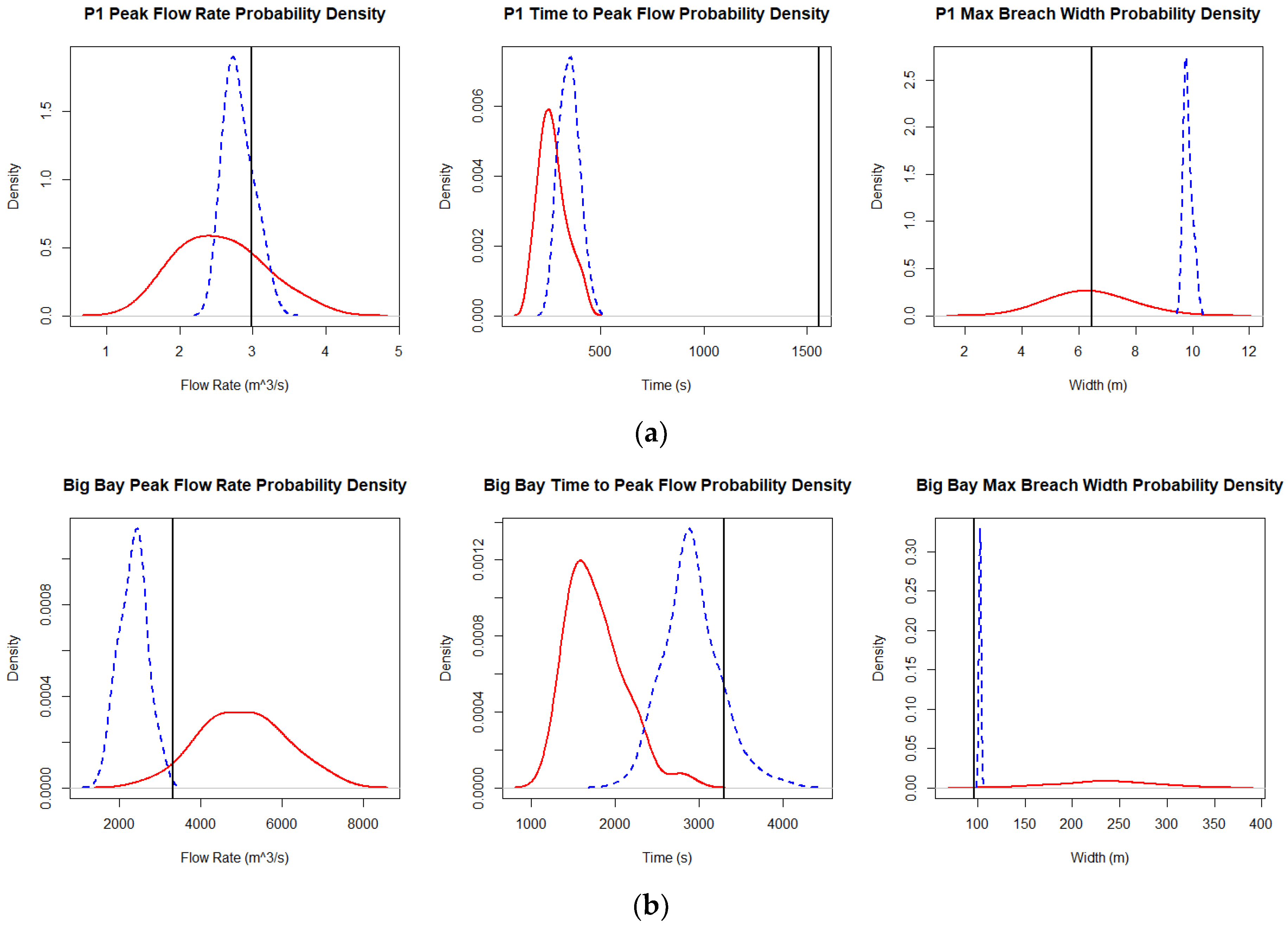
For the uncertainty analysis, comparisons are drawn both between models and between the scales of the dams using the observational measurements as a frame of reference. Figure 2 provides plots of the probability densities of the output metrics. To quantify the relationships between densities, Table 3 provides the range, mean, median, mode, and standard deviation for these densities.
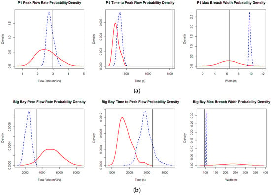
Figure 2.
(a) HERU P1 and (b) Big Bay probability density plots. The red solid line is DLBreach and the blue dotted line is WinDAM C.

Table 3.
DLBreach and WinDAM C probability density characteristics. Mean, median, and mode also include their percent errors to the observed measurements.
When examining the differences between the models, WinDAM tends to more closely match the observed measurements. This is sometimes even the case when the observed measurement does not fall within the range of outputs from the model. WinDAM also tends to have higher average values, particularly for P1 results. In terms of certainty, WinDAM tends to have narrower ranges and standard deviations. However, there are also similarities as both models underestimate the peak flow rate for P1 and the time to peak for both dams. They overestimate the breach width for Big Bay, but WinDAM C is more accurate.
When comparing scales, WinDAM provides a better estimate of the peak flow rate at the small scale and better estimates of the time to peak and breach width at the large scale. DLBreach, on the other hand, only provides a good estimate of the breach width at the small scale. In general, the percent errors for both models worsen for the peak flow rate, and they improve for the time to peak flow as the scale increases.
3.2. Variance
Table 4 provides the statistical significance of the parameters for the output metrics. Significance is defined as a p-value less than 0.05, meaning that there is a less than 5% chance that the same results would occur otherwise. Of the most significant results, the soil erodibility, water level, and initial height of the breach highly influence the output metrics in both models and dams. This is not surprising as these parameters and metrics were identified as notable in previous phases. There are also some trends specific to certain models or dams. For DLBreach, soil diameter is relatively significant overall, while dam height is significant for the peak flow rate and max breach width. For Big Bay, it would appear that the crest width and initial breach diameter are significant for the metrics. Finally, there are extremely specific results, such as the dam height being significant for time to peak flow, in the HERU P1 scenario.

Table 4.
Parameter significance for P1 DLBreach, P1 WinDAM C, Big Bay DLBreach, and Big Bay WinDAM C. “O”, “x”, and “-“ are used to mean the parameter is either significant (p < 0.05), not significant, or not used for that scenario, respectively.
3.3. Optimization
The four optimization methods are evaluated based on their use. The first method is provided with the uncertainty analysis, and so its focus is on how the relationship between the inputs and outputs of an individual run can supplement the relationship found as a whole. The Dakota method by comparison focuses on the absolute limits of the relationship between the results and the observed measurements. The last two methods utilize machine learning, and so they focus on the efficiency of obtaining the results.
3.3.1. Ranked Uncertainty Runs
The probability density results provide an idea of the overall behavior of the models. However, these results are detached from the capabilities of any particular run. That is, it is not clear how close any single run is to matching the peaks of these distributions, and more importantly, how close any single run is to matching the observed measurements. For this purpose, investigating the performance of individual runs is necessary to understand this relationship.
The performance function provided as part of the initiative is calculated for every run of each dam/model pair. Table 5 provides the scores for the top five runs. There is a clear difference between scales and models. These scores show that individual runs for the larger dam are significantly closer to the observed measurements. It can also be seen that WinDAM C generally has a smaller difference. The difference between this observation and that of the uncertainty run is the difference between the majority of runs collectively being closer versus the best individual runs being closer. To break down these results, Table 6 provides the percent error of the output metrics for the top-scoring runs. As can be seen, these errors are quite high, thus explaining some of the higher scores. These values support some of the earlier observations, but we also see that time to peak in particular is especially different from the observed measurements.

Table 5.
Top five runs for each scenario/model pair based on performance function score.

Table 6.
Percent error of output metrics compared to their measured values for top-ranked runs.
While the model outputs are the main interest in such an investigation, it is also useful to investigate the inputs. By examining where these values lie in their ranges and how they compare to the provided inputs, we can complete our understanding of how these models function in comparison to the system they are modeling. Table 7 provides the percent error of the inputs compared to their provided values. Of particular interest here is how far off certain parameters, such as the reservoir volume for the Big Bay scenarios, are from their provided values. This might suggest that the measurements are off, or that the models do not accurately reflect the impact of these parameters in their equations.

Table 7.
Percent error of input parameters compared to their estimates for top-ranked results.
While looking at the single best scores for each scenario provides an idea of the upper limit of performance, extending the view reveals additional patterns. Here, we focused on the distributions of input parameters and output metrics formed from those runs, which scored in the top 25%. Comparing these distributions to those of the full set of runs we see that, on average between the four scenarios, the range of values for erodibility is about 30% that of the provided range. Other parameters, such as crest height and width, as well as water levels, use around 60% of their ranges. These are generally much narrower than the other parameters, which use 90–100% of their ranges. This could further support some of the variance and sensitivity results in suggesting that those parameters with narrower ranges have a greater influence. Of course, there are other factors that could explain this clustering effect, such as the sizes of the provided ranges and the number of runs performed for each scenario.
3.3.2. Pattern Search
As outlined earlier, an asynchronous pattern search was used for a more rigorous optimization method. Table 8 provides the results from this experiment. Provided are the average percent errors and performance function scores for the results of each parameter set found. Additionally, a set of percent error calculations using only the performance score metrics is included to allow a better comparison between the two optimized sets.

Table 8.
Dakota optimization experiment results. Each column represents the results from a different set of inputs to their respective model.
It is important to note that the estimates provided with the initial data result in neither the best performance score nor average percent error. This matches the results found earlier with the density graphs, and provides another metric for quantifying those differences.
What these results demonstrate is that the choice of which output metrics to optimize clearly matters. What is harder to determine is the effect that the formulation of the objective functions has on the parameters that are found. A better comparison could be performed if the average percent error of the performance function metrics was used as the alternative objective function instead of the average error of all output metrics.
Aside from comparing the outputs, we can also compare the different sets of parameters that were found. The parameters that are most similar between the two suggested sets include dam height, erodibility, water level, Manning’s coefficient, particle diameter, and friction angle. From this, and the earlier variance evaluations, we can infer there are likely two reasons for this pattern. For one, those parameters with a strong influence will greatly change the results for any small change in the parameter value. Therefore, to obtain optimal results, regardless of the differences in the two objective functions, these values are limited to a small range of possibilities. On the other hand, if a parameter has little to no influence, then there is no reason to change its value. What we are left with are likely parameters that have a medium effect on the results and thus can be tweaked to optimize for one objective over another.
This also provides another method of comparing models and the effects of embankment size. Once again, we see some of the same patterns present in the uncertainty and rankings analyses. Generally, it would seem that WinDAM C produces lower average percent errors and better performance scores. This is expected at this point, but something else that also appears in these results, and perhaps is clearer here, is the difference in scales. At the small scale, different parameters are changed between functions. For WinDAM, the percent error and performance scores are generally worse at the smaller scale. Some of this difference may be due to differences in the error of measurement between the two models.
3.3.3. Regression Models
During the investigation, multiple methods for optimization were explored. While the use of Dakota is presented here as the final result, the findings from the other methods may still be of interest. In particular, there is the question of whether machine learning is suitable for this field. If care is taken to formulate the problem in a suitable manner, then it would appear that machine learning is capable of capturing some of the underlying features of these systems.
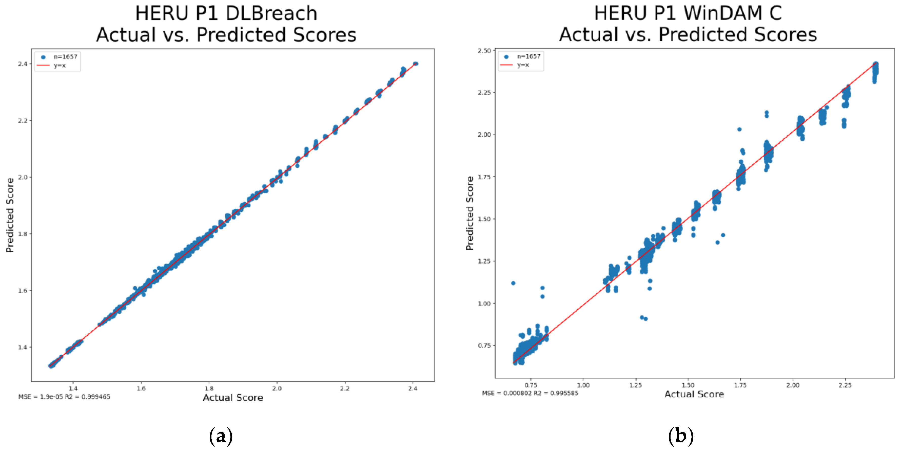
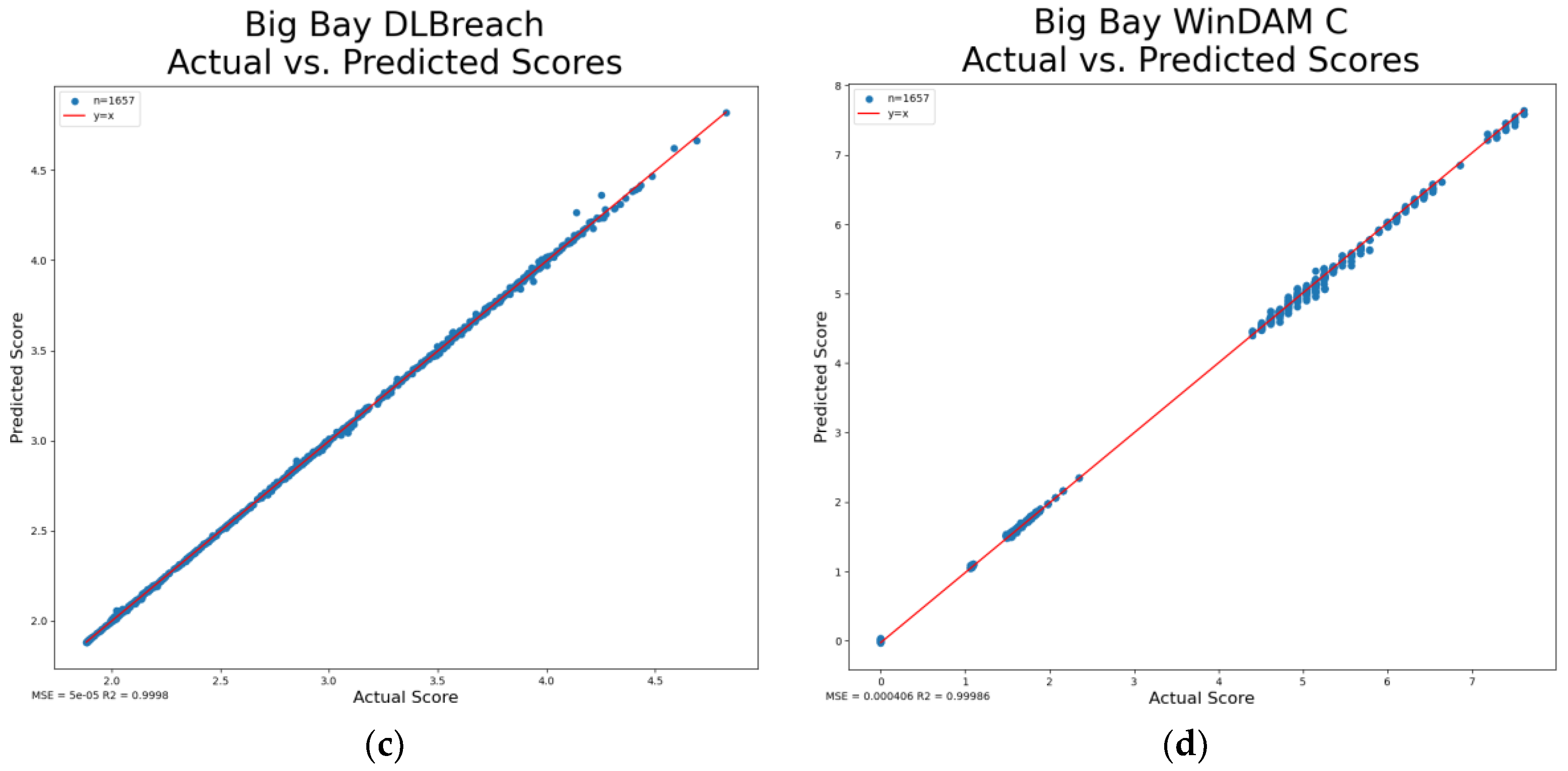
As outlined in the methodology, both methods used regression models trained on regularly spaced samples of the parameter space. Figure 3 shows the graphs for the fit of regressions models trained on the performance scores for each of the four scenarios. Provided in the caption are the mean squared errors and R2 values. As can be seen, there is a strong relationship between the predicted value and actual value suggesting promising results for an optimization search.
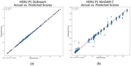
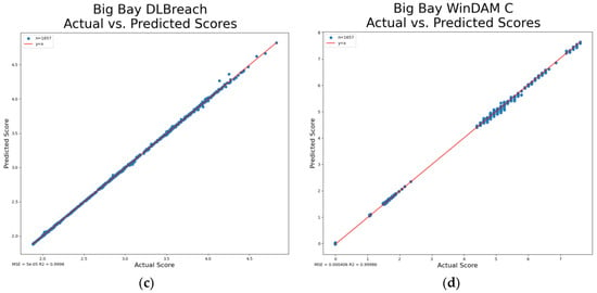
Figure 3.
Regression model Perf1 scores vs predicted Perf1 scores for (a) HERU P1 DLBreach (MSE = 0.000019, R2 = 0.99946), (b) HERU P1 WinDAM C (MSE = 0.0008, R2 = 0.99558), (c) Big Bay DLBreach (MSE = 0.00005, R2 = 0.9998), and (d) Big Bay WinDAM C. (MSE = 0.0004, R2 = 0.99986).
Table 9 provides the percent error of output metrics for the parameters suggested by the reverse, surrogate, and Dokota methods. Only Big Bay is shown here as these last two methods are meant as a simple demonstration. While the results for the reverse function shown here appear relatively similar to the other two methods, it should be noted that this was a kind of best-case scenario. Other attempts of using this method are fraught with complications that will be discussed later. Instead, the similarity between the results of the surrogate model with dual-annealing vs the original models with the Asynch pattern search are of greater interest. It should be noted that pattern search is a local method while dual-annealing is a global method, which can contribute to some of the poorer performances of the Dakota results.

Table 9.
Big Bay metric percent errors for the parameter sets achieved by three different optimization methods.
4. Discussion
The results from these experiments are meant to be interpreted in conjunction with the work performed by the other modelers, but there are still some conclusions that can be drawn from this work alone. While the patterns within the data have been highlighted, their potential causes have not been addressed.
The designers of these models have to make decisions on how to abstract the features of the complex systems they wish to model. How the models are used plays a part in guiding how these decisions are made. For instance, WinDAM C is used by professionals to design and test safe embankments. When the matter of liability is involved, it is safer to assume that something will fail sooner and “worse”. Given a scatter plot of embankment qualities to failure statistics, a prediction function designed to encompass these points will be closer to some than others. This relationship may then explain some of the discrepancies seen in the uncertainty results.
Important decisions like this are not limited to the designers; both modelers and data gatherers are subject to this process. As an example, modelers are provided a single input to represent the height of a dam, but earthen dams are not always perfectly uniform across their crest. Another example is the materials used for the dams; both models assume a homogeneous soil, but some dams are made with different layers or with a unique core. One way of addressing these differences in our models is the processes demonstrated here. This does not perfectly replicate the effects of a slump in a dam or a core of a different material, but we hope that the distributions of the results approximate reality in some way. For data gatherers, one of the decisions they make is when to start measuring time. The models also have their own start time, and the discrepancy between these two starting points can explain some of the high errors for the time-related metrics. Regardless of how they perform individually, there is also the question of how the models and dams compare.
The results seem to suggest that, in a number of ways, WinDAM C more closely matches the measured values for these failure events. Furthermore, the scale of the dam also contributes to accuracy as Big Bay produced better results for some metrics while P1 did so for others. Seeing as there are only two examples though, it is difficult to determine if the results both between models and between scales are typical.
In terms of the variance analysis, the results from this portion are complicated by several factors. For a start, while the distributions of the metrics closely resemble normal distributions, they contain anomalous features, which may prevent them from being true normal distributions. Since an ANOVA of this type typically requires a normal distribution, it is uncertain the degree to which these “bumps” affect that. Some of these bumps may be caused by violations of relationships between the input parameters. Factors such as erodibility and cohesion are not fully independent, and unrealistic combinations of values for these are likely to skew the results. These dependent relationships also bring to question the linear function used in the analysis. To improve this, a proper function formulated from the interactions of these parameters would have to be used instead. This, of course, requires knowledge of the domain. Finally, ANOVAs performed in this way assume that the independent variables are categorical, which the input parameters are not. Together, the covariate and continuous natures must be addressed for more accurate results.
Moving on to the optimization results, the dual-annealing technique demonstrates the efficacy of the surrogate model technique for this domain. However, as employed here, it comes at the cost of the work to train the model. More practical methods exist, including those implemented in Dakota, if parameter optimization is the only desire. More importantly, it demonstrates that the behavior of the models can be replicated with these techniques. This suggests that it may be feasible to train regression models’ historical and laboratory data to attempt to capture the intricacies that may be lost in our manually-developed models.
The inverse function approach on the other hand demonstrates the issues with the poor adaptation of machine learning techniques. The goal with this approach is to obtain a simple model that can be fed the desired output metrics and receive input metrics as a result. In order for such a method to work as intended, there needs to be a one-to-one relationship between inputs and outputs for the original function such that it is reversible. Such a relationship does not exist for the models trained here. Additionally, we desire the inputs to be within the ranges that are provided, but this method does not have that constraint. Simply clamping to the nearest limit may not necessarily work either depending on the complexity of the underlying function. Finally, this method shows the kind of pitfall that is perhaps most dangerous: it works for one scenario. This can encourage developers to pursue ill-fit options.
5. Conclusions
To summarize, from the uncertainty results and simulation run rankings, we can see that, generally, WinDAM C is more performant for the metrics of interest. Additionally, Big Bay, being representative of the kinds of dams whose data these models were built upon, provides better results in the optimizations. The variance seems to correlate with the known behavior in that parameters such as erodibility and the amount of water have a great influence. Finally, while it may be intentional for the purposes of safety, the accuracy of these models can be rather low. In addition to the margin of error used for safety, a major contributing factor is their simplicity: dams crests are uniform and breaches are straight channels.
Going forward, there are two areas that stand out as potential refinements of this work, the first being a more consistent experimental design. Primarily, it would benefit the comparisons between models and scales, as well as other elements of the analysis, if the parameters used in these simulations were limited to a select subset, which has shown significance in the variance analysis, and which can also be used by all dam/model pairs. From there, a far greater number of simulation iterations may be beneficial for confirming the distributions found here. While something like 500 simulation runs were tested, they showed little difference from the 100 runs. If there are any benefits to be gained, it is likely that the number of runs needs to be in the thousands. From there, the central limit theory will hopefully ensure we obtained well-formed normal distributions. For the optimization sections, the choice of optimization functions is also inconsistent. Perhaps a better comparison might be made between the Perf1 score and the average percent error of only the Perf1 metrics.
The other area of interest might be in exploring the further application of regression models. The use of surrogate models is a known technique and something Dakota is even capable of. The fit of the regression models on just these summary metrics shows promise, but these alone have limited use. Perhaps a more useful application would be training models to accurately recreate the overtime characteristics, such as how the flow rate and breach develop. Supplementing this training with training on data taken from the field may further aid in improving the accuracy. Hopefully, these kinds of models might improve our own understanding of the underlying systems.
Author Contributions
Conceptualization, A.A. and M.N.; methodology, A.A. and M.N.; software, A.A. and M.N.; validation, A.A.; formal analysis, A.A. and M.N.; investigation, A.A.; resources, A.A. and M.N.; data curation, A.A.; writing—original draft preparation, A.A.; writing—review and editing, A.A. and M.N.; visualization, A.A.; supervision, M.N.; project administration, A.A.; funding acquisition: M.N. All authors have read and agreed to the published version of the manuscript.
Funding
This research received no external funding.
Data Availability Statement
Publicly available datasets were analyzed in this study. These data can be found at: https://github.com/amatkinson/P3DamUncertaintyAnalysis, accessed on 3 February 2024.
Acknowledgments
Thank you to the USDA Hydraulic Engineering Research Unit, Stillwater, Oklahoma, for providing the data from their research on erosion.
Conflicts of Interest
The authors declare no conflicts of interest.
References
- CIGBICOLD World Register of Dams. 2024. Available online: https://www.icold-cigb.org/GB/world_register/general_synthesis.asp (accessed on 8 February 2024).
- USACE National Inventory of Dams. 2024. Available online: https://nid.sec.usace.army.mil/#/ (accessed on 8 February 2024).
- Wahl, T.L. Prediction of Embankment Dam Breach Parameters: A Literature Review and Needs Assessment; DSO-98-004; U.S. Dept. of Interior, USBR, Dam Safety Office, Water Resources Research Lab: Denver, CO, USA, 1998. [Google Scholar]
- Thornton, C.I.; Pierce, M.W.; Abt, S.R. Enhanced predictions for peak outflow from breached embankment dams. J. Hydraul. Eng. 2010, 15, 338–349. [Google Scholar] [CrossRef]
- Fread, D.L. DAMBRK: The NWS Dam Break Flood Forecasting Model; National Weather Service Report; NOAA: Silver Spring, MD, USA, 1984. [Google Scholar]
- Fread, D.L. Breach: An Erosion Model for Earthen Dam Failures; National Weather Service; NOAA: Silver Spring, MD, USA, 1988; (rev. 1991). [Google Scholar]
- Hassan, M.; Morris, M.; Hanson, G.; Lakhal, K. Breach formation: Laboratory and numerical modeling of breach formation. In Proceedings of the Association of State Dam Safety Officials Annual Meeting, Phoenix, AZ, USA, 26–30 September 2004; ASDSO: Lexington, KY, USA, 2004. [Google Scholar]
- Wahl, T.L.; Lentz, D.J. Physical Hydraulic Modeling of Canal Breaches; USBR Hydraulic Laboratory Report HL-2011-09; U.S. Dept. of Interior, USBR, Dam Safety Office, Water Resources Research Lab: Denver, CO, USA, 2011. [Google Scholar]
- Al-Riffai, M. Experimental Study of Breach Mechanics in Overtopped Noncohesive Earthen Embankments. Ph.D. Dissertation, University of Ottawa, Ottawa, ON, Canada, 2014. [Google Scholar]
- Ashraf, M.; Soliman, A.H.; El-Ghorab, E.; Zawahry, A.E. Assessment of embankment dams breaching using large scale physical modeling and statistical methods. Water Sci. 2018, 32, 362–379. [Google Scholar] [CrossRef]
- Alvarez, T.; Valente, S.; Amaral, S.; Viseu, T.; Ferreira, R.M. Sensitivity analysis to the pilot channel geometry in dam breach by overtopping. In Proceedings of the 28th IAHR World Congress, Graz, Austria, 22–27 August 1999. [Google Scholar] [CrossRef]
- Temple, D.M.; Hanson, G.J.; Neilsen, M.L.; Cook, K.R. Simplified breach analysis for homogeneous embankments: Part 1, Background and model components. In Proceedings of the U.S. Society on Dams. Technologies to Enhance Dam Safety and the Environment, Salt Lake City, UT, USA, 6–10 June 2005; USSD: Westminster, CO, USA, 2005; pp. 151–161. [Google Scholar]
- Hanson, G.J.; Tejral, R.D.; Hunt, S.L.; Temple, D.M. Internal erosion and impact of erosion resistance. In Proceedings of the 30th U.S. Society on Dams Conference, Sacramento, CA, USA, 12–16 April 2010; USSD: Westminster, CO, USA, 2010; pp. 773–784. [Google Scholar]
- Hunt, S.L.; Temple, D.M.; Neilsen, M.L.; Ali, A.; Tejral, R.D. WinDAM C: Analysis Tool for Predicting Breach Erosion Processes of Embankment Dams Due to Overtopping or Internal Erosion. ASABE Appl. Eng. Agric. 2021, 37, 523–534. [Google Scholar] [CrossRef]
- Vaskinn, K.A.; Lovoll, A.; Hoeg, K.; Morris, M.; Hanson, G. Physical modeling of breach formation: Large scale field tests. In Proceedings of the Association State Dam Safety Officials Annual Meeting, Phoenix, AZ, USA, 26–30 September 2004; ASDSO: Lexington, KY, USA, 2004. [Google Scholar]
- Hanson, G.J.; Cook, K.R. Apparatus, test procedures, and analytical methods to measure soil erodibility in situ. Appl. Eng. Agric. 2004, 20, 455–462. [Google Scholar] [CrossRef]
- Hanson, G.J.; Cook, K.R. Determination of material rate parameters for headcut migration of compacted earthen materials. In Proceedings of the Association State Dam Safety Officials Annual Meeting, Phoenix, AZ, USA, 26–30 September 2004; ASDSO: Lexington, KY, USA, 2004. [Google Scholar]
- Hanson, G.J.; Hunt, S.L. Lessons learned using laboratory JET method to measure soil erodibility of compacted soils. Appl. Eng. Agric. 2007, 23, 305–312. [Google Scholar] [CrossRef]
- ASCE/EWRI Task Committee on Dam/Levee Breaching. Earthen embankment breaching. J. Hydraul. Eng. 2011, 137, 1549–1564. [Google Scholar] [CrossRef]
- CEATI. Evaluation of Numerical Models for Simulating Embankment Dam Erosion Breach Processes; U.S. Dept. of the Interior, Bureau of Reclamation, Dam Safety Development Program, Report No. DSO-2017-02; CEATI International Working Group on Embankment Erosion and Dam Breaching: Montreal, QC, Canada, 2017. [Google Scholar]
- Floodsite. HR Breach Model. 2020. Available online: http://www.floodsite.net/html/HR_Breach_Model.htm (accessed on 15 July 2023).
- Zhong, Q.; Wu, W.; Chen, S.; Wang, M. Comparison of simplified physically based dam breach models. Nat. Hazards 2016, 84, 1385–1418. [Google Scholar] [CrossRef]
- Wu, W. Simplified physically based model of earth embankment breaching. J. Hydraul. Eng. 2013, 139, 837–851. [Google Scholar] [CrossRef]
- West, M.; Morris, M.; Hassan, M. A Guide to Breach Prediction; HR Wallingford: Wallingford, UK, 2018. [Google Scholar] [CrossRef]
- Zhong, Q.M.; Chen, S.S.; Deng, Z.; Mei, S.A. Prediction of overtopping-induced breach process of cohesive dams. J. Geotech. Geoenviron. Eng. 2019, 145, 04019012. [Google Scholar] [CrossRef]
- Yochum, S.E.; Goertz, L.A.; Jones, P.H. Case study of the big bay dam failure: Accuracy and comparison of breach predictions. J. Hydraul. Eng. 2008, 134, 1285–1293. [Google Scholar] [CrossRef]
- Wu, W. Introduction to DLBreach a Simplified Physically-Based Dam/Levee Breach Model; Technical Report; Department of Civil and Environmental Engineering, Clarkson University: New York, NY, USA, 2016; p. 119. [Google Scholar]
- Adams, B.; Bohnhoff, W.; Dalbey, K.; Ebeida, M.; Eddy, J.; Eldred, M.; Hooper, R.; Hough, P.; Hu, K.; Jakeman, J.; et al. Dakota, a Multilevel Parallel Object-Oriented Framework for Design Optimization, Parameter Estimation, Uncertainty Quantification, and Sensitivity Analysis: Version 6.15 User’s Manual; Sandia National Laboratory: Albuquerque, NM, USA, 2021. [Google Scholar] [CrossRef]
- Neilsen, M.; Cao, C. Coupled Dam Safety Analysis using BREACH and WinDAM. In Proceedings of the 15th International Conference on Scientific Computing, Las Vegas, NV, USA, 15–17 March 2017; pp. 82–85. [Google Scholar]
Disclaimer/Publisher’s Note: The statements, opinions and data contained in all publications are solely those of the individual author(s) and contributor(s) and not of MDPI and/or the editor(s). MDPI and/or the editor(s) disclaim responsibility for any injury to people or property resulting from any ideas, methods, instructions or products referred to in the content. |
© 2024 by the authors. Licensee MDPI, Basel, Switzerland. This article is an open access article distributed under the terms and conditions of the Creative Commons Attribution (CC BY) license (https://creativecommons.org/licenses/by/4.0/).

