Abstract
The role of the Manning roughness coefficient in modifying a tsunami time series of flow depth inundation was studied in Iquique, Chile, using a single synthetic earthquake scenario. A high-resolution digital surface model was used as a reference configuration, and several bare land models using constant roughness were tested with different grid resolutions. As previously reported, increasing the Manning n value beyond the standard values is essential to reproduce mean statistics such as the inundated area extent and maximum flow depth. The arrival time showed to be less sensitive to changes in the Manning n value, at least in terms of the magnitude of the error. However, increasing the Manning n value too much leads to a critical change in the characteristics of the flow, which departs from its bore-like structure to a more gradual and persistent inundation. It was found that it is possible to find a Manning n value that resembles most features of the reference flow using less resolution in the numerical grids. This allows us to speed up inundation tsunami modeling, which could be useful when multiple inundation simulations are required.
1. Introduction
Tsunamis have the potential to cause widespread damage and loss of life over large swaths of coastal areas. As a first step to mitigate their effects, an accurate and detailed assessment of the hazard is essential. Typically, this is carried out through forecasting the Tsunami Intensity Metrics (TIMs) relevant to the problem of interest by using numerical modeling of the tsunami, subject to initial and boundary conditions. While it is typically assumed that the initial condition, that is, the tsunami source, is the dominant parameter that allows for distinguishing between the hazard posed by different events, e.g., [1], the boundary conditions play a significant role in controlling the magnitude of the flow if the initial condition remains constant. Chief among these are the topography and bathymetry over which the flow is expected to occur, which control the flow to first order based on their gradients and absolute size, which induce normal stresses on the flow. However, the characteristics of the terrain also affect the flow by inducing dissipation directly through bottom friction as shear stress. Whereas the inclusion of the former is relatively straightforward, the inclusion of the latter requires a model for the stresses. The inclusion of this effect is achieved by one of the few free parameters in the numerical modeling of tsunamis.
Whereas much effort has been carried out to reduce the uncertainty in the initial and boundary conditions—see, for recent reviews [2,3]—the study of the dissipation model has been analyzed only occasionally. Moreover, most of the analysis has focused on the effect of the dissipation term in tsunami inundation metrics such as the extent of the inundated area, and extreme statistics for flow depth. Other quantities, such as the arrival time and/or the shape of the time series of inundation, have not been analyzed. These can be relevant for evacuation studies, or the assessment of the flow characteristics for infrastructure design.
This work aims to complement this existing understanding by analyzing the effect of varying the single free parameter pertaining the dissipation in the modeling of tsunamis using the non-linear shallow water equations, with a special focus on its effect on the arrival time. To this end, in the following section, an overview of the approaches used to date is provided. Next, Section 3 introduces the methodology used, followed by its results in Section 4. A discussion of the implications is provided in Section 5, followed by the conclusions.
2. Background
The mathematical modeling of tsunamis can be carried out in various ways, but the most frequent of these are based on the non-linear shallow water equations, e.g., [4,5]:
where g is the acceleration due to gravity, is the free surface disturbance above the mean surface (z = 0), , are the horizontal components of the vertically averaged velocity field , B is the local depth (i.e., the bathymetry), and represents source and sink terms. In these equations, spatial derivatives consider only horizontal terms, and z points upwards. Here, the inclusion of dissipation through friction in can be performed by modeling the bottom shear stress per unit of mass in terms of an appropriate formulation. The most frequent choice is to adopt Manning’s model:
which was proposed for steady, uniform flow conditions in open channels [5,6]. Here, u is the magnitude of the velocity (the flow speed), and is the hydraulic radius. For a section of infinite width, . The nonlinear dependency on depth means that the effect of this term becomes negligible for depths larger than B > 50 m [7], but it can become a dominant term in very shallow water; for instance, during the inundation phase of the tsunami. The remainder parameter, n, is known as the Manning value, which is an empirical parameter that is the inverse of the proposed by Kutter, who, in turn, had proposed it to simplify the estimation of friction when compared with Chezy’s formula, which required two parameters. Due to the nature of Equation (2), n is a dimensional number, with units . Alternatively, the Manning value can be referred to as [8,9], but it leads to the same problem as Kutter’s value, where greater friction is associated with a smaller M value, making it counter-intuitive. It is noted that, in Equation (2), n is a free parameter.
Whereas the development and subsequent use of the Manning equation for open channel flows (both natural and artificial) have benefited from extensive calibration leading to well-established n values and procedures for its estimation, the calibration for tsunami modeling has been rather limited. Bricker et al. [6] noted that most of it stems from a single work, that of Kotani et al. [10], which is available only in Japanese. In most situations, modelers use standard values for n, which appear to have been passed along as tradition more than anything. The most common is n = 0.025 , which Kotani et al. [10] indicate as appropriate for riverine and coastal areas, whereas Kaiser et al. [8] and Gayer et al. [11] support its use because it is associated with soils covered by coarse sand, and assign it to streets, beaches, and bare soil. In contrast, Muhari et al. [12] indicate that it was originally derived for natural channels in good condition. It is noted that the use of Manning’s equation in open channel cases assumes the flow to be hydraulically rough, as is the case for tsunamis at peak inundation flow depths and speeds.
However, there are sources of roughness that can be relevant for tsunami flows also, such as trees, buildings, and infrastructure, whose inclusion might vary depending on the discretization of the domain. The large spatial extent of inundation zones imposes the a priori definition of a modeling strategy for friction. Ideally, if computational resources were abundant, the model could consider a resolution large enough to model structures and buildings as being resolved by the grid; hence, the flow would accommodate around it. Buildings are assumed to be able to withstand the forces from the tsunami; therefore, they remain as fixed features throughout the simulation. Moreover, they are treated as impermeable, thereby effectively altering flow patterns and inducing energy losses through this. Kaiser et al. [8] term this approach as buildings as elevation data, and others call it topography model [12,13]. It is noted that this can be a misnomer, as, in reality, what is being used as the input is a Digital Terrain Model (DTM) over which the building elevation is overlaid, leading to a Digital Surface Model (DSM) [14], which is the preferred term to be used here.
However, computational resources are often limited, leading to a reduced spatial resolution. Hence, features such as buildings, roads, forests, and other features can become smaller than the grid size. These could lead to an apparent increase in sub-grid roughness than needs to be accounted for by using an Equivalent Roughness Model (ERM) [12], where these features are modeled by larger Manning n values, using, as a reference, a DTM for the topography. These n values can be determined using expert judgment [11], or by adopting a model originally devised for the inclusion of vegetation in riverine flows [15] to include land use and building conditions [8,12,16,17]. The model reads, e.g., Koshimura et al. [17]
where is a reference Manning value, is a drag coefficient, l is a horizontal scale of the section under study, and represents the fraction of land used by vegetation (or buildings). Thus, this model modifies the reference Manning value to account for the drag of existing elements within the grid cell. Implementing this formulation requires, aside from the standard problem of prescribing the reference value , a highly detailed assessment of the area covered by infrastructure and an estimation of its drag properties, which has seldom been available. Other names for this approach are buildings as roughness [8], or the equivalent-n model [13].
If the numerical model allows it, these values can be passed on as spatial maps of the Manning n value, varying from cell to cell (Variable Roughness Model, VRM), but models typically only allow for a single value of n for the entire domain. Muhari et al. [12] define this type of configuration as Constant Roughness Models (CRM). This terminology is retained here.
Therefore, considering the combination of how the Manning n value is estimated and how it is included in the model, it is possible to use DSM, CRM-ERM, VRM-ERM, and expert judgment CRM or VRM implementations. The comparison between these approaches has been studied in recent years, noting that there is a close relationship between the grid size and the value of the Manning n value. The use of high-resolution topography and bathymetry also leads, at least in principle, to a more accurate modeling [11,18,19]. The overall conclusion is that inundation TIMs, such as runup, inundation extent, and maximum flow depths, are influenced by the choice of the Manning n value [6,8,12,14,16,20]. The standard values of n used in CRM modeling lead to an overestimation of the inundation extent and flow depths, and also of momentum fluxes. These TIMs are essential for most hazard assessments. On the other hand, Gayer et al. [11] found no significant differences between the CRM-ERM and VRM-ERM regarding flow depths.
These studies appear to suggest that the use of the Manning n value based on riverine or open channel flow dissipation rates is not consistent with the type of sub-grid roughness and dissipation that is induced by the built environment. Higher values for the Manning n value are thus needed to simulate this enhanced roughness. It can be argued, then, that a balance can be found, where models using lower grid resolutions can yield similar results to those at a higher resolution, provided that a suitable Manning n value is used. In this sense, the Manning n value could become an efficiency term, or calibration parameter, rather than an actual physical quantity. It is noted that this notion is the reason for why the parameter is termed herein the Manning n value, instead of Manning friction or the roughness coefficient, e.g., [6,14], which points to a more physical explanation. Regardless, a potential benefit of finding such a balance is that faster computational times could be achieved, which could be beneficial if a large number of simulations is required. Muhari et al. [12] tested these ideas and were able to find a balance, especially on gradually varying topography, when the target TIM was the flow depth. However, the problem lies in the flow velocity. The use of actual data for the built environment forces a geometrical alteration of the possible pathways that the flow can encounter, which leads to flow focusing on streets, for instance. The analysis of flow velocities, and, consequently, of momentum fluxes, has shown that there is no substitute for the DSM if these are the TIMs of interest [8,9,12], unless a modification is introduced to the overall model, such as the porous body model [13].
Most of these analyses are carried out by assessing time-integrated TIMs, such as their extrema, where the effect of time is disregarded. Yamashita et al. [13] found that the use of the different models retains the temporal structure of the flow depth , but with significant differences in the velocity . However, the error in arrival time did not exceed 50 s, when the first arrival occurred around 2400 s; that is, 2%.
Tsunami arrival times and the temporal structure of the flow can be relevant for other types of studies. Evacuation studies, for instance, especially those that involve agent-based modeling, e.g., [21,22,23,24,25], use tsunami modeling results as an input to assess evacuation success rates. However, rather than standard TIMs, such as the flow depth time series , the relevant parameter is whether . When the flow depth exceeds a given threshold for the first time, it indicates that a nearby agent would be reached by the tsunami and, therefore, it is considered a casualty. This is a relevant aspect because it can be argued that it is not required to match flow features such as its maximum, just its temporal occurrence. On the other hand, it is essential to have a proper assessment of the inundation extent, so as to evaluate where safe zones are located. These two goals appear as contradictory to the modeler. For the former, modeling runs with coarse grids could suffice, but, for the latter, a high resolution and precise values of the Manning n value would be required instead. This has prompted most of these evacuation studies to use a single, computationally intensive, tsunami model at a high resolution [23]. The downside of this approach is that it limits the assessment of evacuation strategies for multiple scenarios and/or conditions.
This work stems from this apparent conundrum: whether simpler scenarios can reproduce the flow characteristics relevant for evacuation studies by means of an appropriate choice of model parameters, such as the Manning n value. Thus, this is a primary step toward evaluating whether evacuation studies can be improved by using multiple tsunami scenarios. A second objective is to assess whether a net gain in terms of computational time, at the expense of precision in other TIMs, can be achieved without affecting TIMs relevant for evacuation modeling.
3. Materials and Methods
The methodology involves the comparison of numerical modeling results of inundation using a range of Manning values, grid nesting schemes, and discretization sizes. While the approach can be used anywhere, the city of Iquique, Chile (2012′51″S 70109′09″) was used as the test site. Iquique is located just in front of the so-called Northern Chile seismic gap [26]. From a modeling perspective, Iquique has several relevant features that could be of interest. It is located over a relatively narrow coastal plain that is flanked by a low-elevation coastal range. The coastline of Iquique alternates between low-lying areas in the northern section and a coastal terrace that lies 4-5 m above mean sea level, towards the south. The low-lying areas were barely inundated during the 8.2 2014 Pisagua earthquake and tsunami [27,28], though a large event occurred in 1877 [29,30]. Prior hazard assessments suggest that the northern section of the city can have larger inundation as it resembles more of an inundation floodplain, whereas the southern section is narrower and steeper [31]. Iquique is placed in front of a narrow section of an otherwise wide continental shelf, thus making it susceptible to short period resonance [32]. The presence of both wider and narrower coastal sections allows for studying the effects of roughness parameters over inundation, which are more relevant when slopes are gentle and the inundation extent is large [33,34].
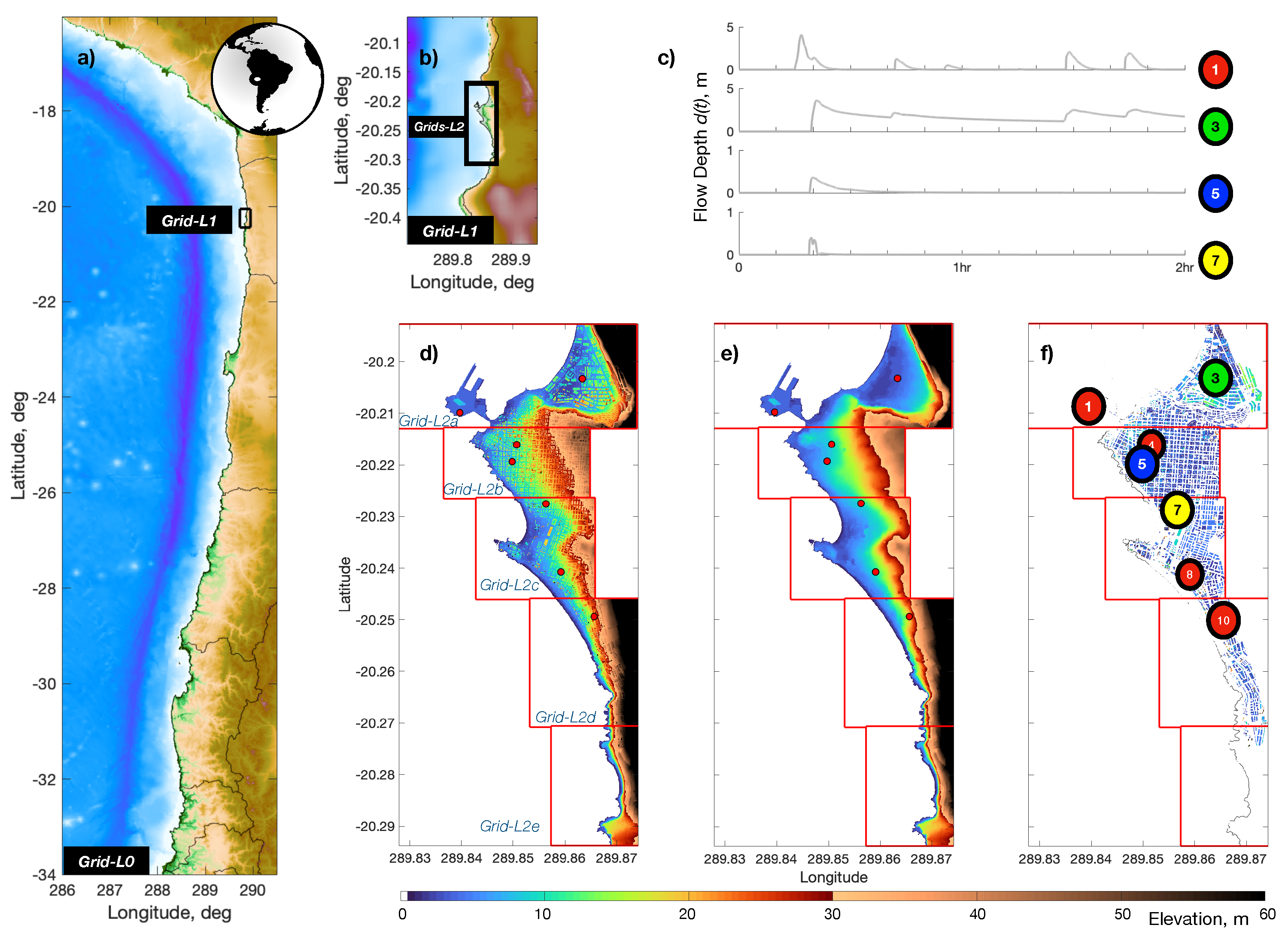
The inundating flows were estimated using the numerical NLSWE model Tsunami-HySEA, which has been benchmarked and validated in accordance with U.S. National Tsunami Hazard Mitigation Program (NTHMP) [35,36], as well as for currents [37]. Up to four sets of nested grids, with varying spatial resolutions, were built from the freely available General Bathymetric Chart of the Oceans [38] and nautical charts elaborated by the Hydrographic and Oceanographic Service of the Chilean Navy (SHOA). Inland topography was determined from LiDAR flights that allowed for the construction of DSM and DTM surfaces (Figure 1). Three nesting schemes were tested in order to assess the effect on the final inundation map of the nesting scheme. The outermost and coarsest layer was built from GEBCO data using a resolution of 30 arcsec (roughly 900 m). Two telescopic levels were used, which were defined by the ratio between the parent and child grids. Ratios of 4 and 8 were used, using three configurations as shown in Table 1, which allowed for a maximum grid resolution of 3.51 m per side. Figure 1 shows the extent of each of the Cartesian numerical domains. In the latest grid level, streets and buildings were included for the baseline DSM model, assuming that buildings were fully resistant to the incoming flows, and remained in place during the modeling of the reference simulation (Figure 1d), whereas, in all others, the bare surface was retained (Figure 1e). Buildings were assumed to be taller than the maximum flow depth; hence, they are never covered by the flow for this reference scenario. For the other cases, buildings were removed while streets retained the elevation leading to DTM cases, as shown in (Figure 1f). This allowed for the comparison between DSM, and DTM-CRM results, as the version of Tsunami-HySEA tested did not allow for a VRM.
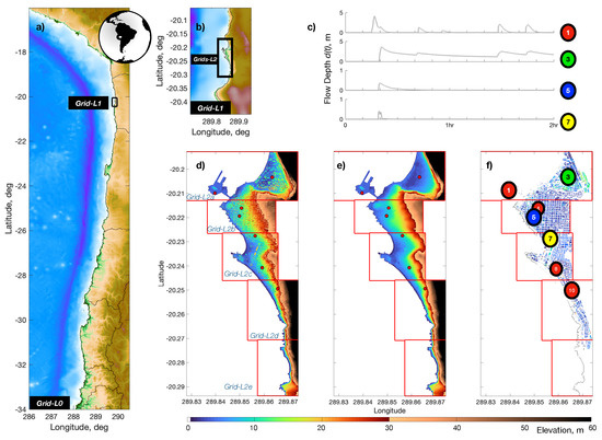
Figure 1.
Location of the area of interest and coverage of the numerical grids. (a) Outermost domain, Level-0; (b) Intermediate domain, Level-1; (c) Time series at gauges of interest; (d–f) Five different Level-2 grids, shown as (d) DSM, (e) DTM, and (f) the difference between DSM and DTM. In (d–f), the difference in color maps is at 30 m elevation. Colored dots denote the location of the inland gauges. These colors are retained in all figures to identify each inland gauge.

Table 1.
Vectors of the ratio of grid resolution tested.
Owing to the computational burden imposed by the high resolution used, the inundation zone was divided into five different grids, each of them modeled in accordance with the ratios shown before. These are shown in Figure 1d–f. The three grids further north are of interest because they differ in terms of urban density and the type of structures. The northernmost is located over a floodplain where buildings are predominantly industrial, with a relatively low building density. The second zone is mainly residential and has small but dense two–three-floor buildings and narrower streets [39]. This distinction could allow for varying Manning n values between grids, but uniform within each grid, as a hybrid CRM-VRM model. However, since no other information was available to allow for quantifying the difference between grids, this was not explored further.
A total of 39 model runs were considered for each of the thee ratios using 13 Manning n values. These range from what is considered the reference value, n = 0.025 sm (standard value for tsunami modeling, and used here for the baseline DSM model), up to sm, which has been previously proposed to simulate tsunami resistant buildings, e.g., [8,11,14]. Each of these model runs used DTM-CRM. The tsunami intensity metrics of interest were the maximum inundation area, the map of the maximum flow depth, and the time series at a set of 13 inland numerical gauges, which were located arbitrarily within the domain but ensuring that they were on streets. The first two metrics allow for a basic comparison of the flow characteristics, similar to previous research, e.g., [8,11,14]. The latter allows for comparing the temporal structure of the flow. The approach is thus similar to Muhari et al. [12], but focuses on different TIMs. It is noted that Muhari et al. [12] used a CRM for the baseline case (with a reference Manning n value) and ERM for cases with larger values, which was not tested here.
Finally, the initial condition of the model considered a single earthquake scenario of = 9.0, using a uniform fault model, centered at 70.20829, −21.263962, with dimensions (500; 167) Km, where are the along strike and along dip lengths of the rupture zone. The scenario and its fault parameters were extracted from the database of sources scenarios of the Chilean tsunami warning system [40], and used to model the initial free surface deformation using the Okada [41] formulation. It was assumed that this single scenario suffices for detailing the effects of the boundary conditions on the modeling. Simulations were run for four hours of tsunami time on a cluster with two NVidia K20 m Graphical Processing Units (GPUs). As an additional parameter, the computing wall time was determined from each run.
4. Results
Figure 1c, Figure 2a and Figure 3a show the results of the inundation for the reference modeling, which considered the DSM at the highest resolution using a Manning n value of 0.025. This has been the standard practice, e.g., [31], and it can be argued that streets and bare terrain resemble the assumed conditions for this value. While the extent of the inundation is large, the structure of the time series varies with location within the city. Gauges 1 and 3 show several phases of inundation. Gauge 1 is located on the port peninsula, with a typical early arrival, and it can be subjected to waves overtopping the island but not causing much inundation elsewhere. Gauge 3 shows a steady inundation, with late arriving peaks. This is consistent with the floodplain in the northern part of the city that has been identified to have a high-risk level from earthquakes and tsunamis [31,42]. Gauges 5 and 7 are located in a steeper section of the city, where a denser network of streets and structures exists. This leads to a single inundation cycle, but with different drawdown characteristics among them, as gauge 5 shows a longer retreat phase than gauge 7. The differences in time series are considered sufficient to study the sensitivity of different flow types to varying the Manning n value. In what follows, results will be presented using gauge 3 for the purpose of demonstration, but the analysis is carried out for all gauges. It is of note that the southern gauges (8–10) were not inundated in this simulation.
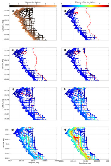
Figure 2.
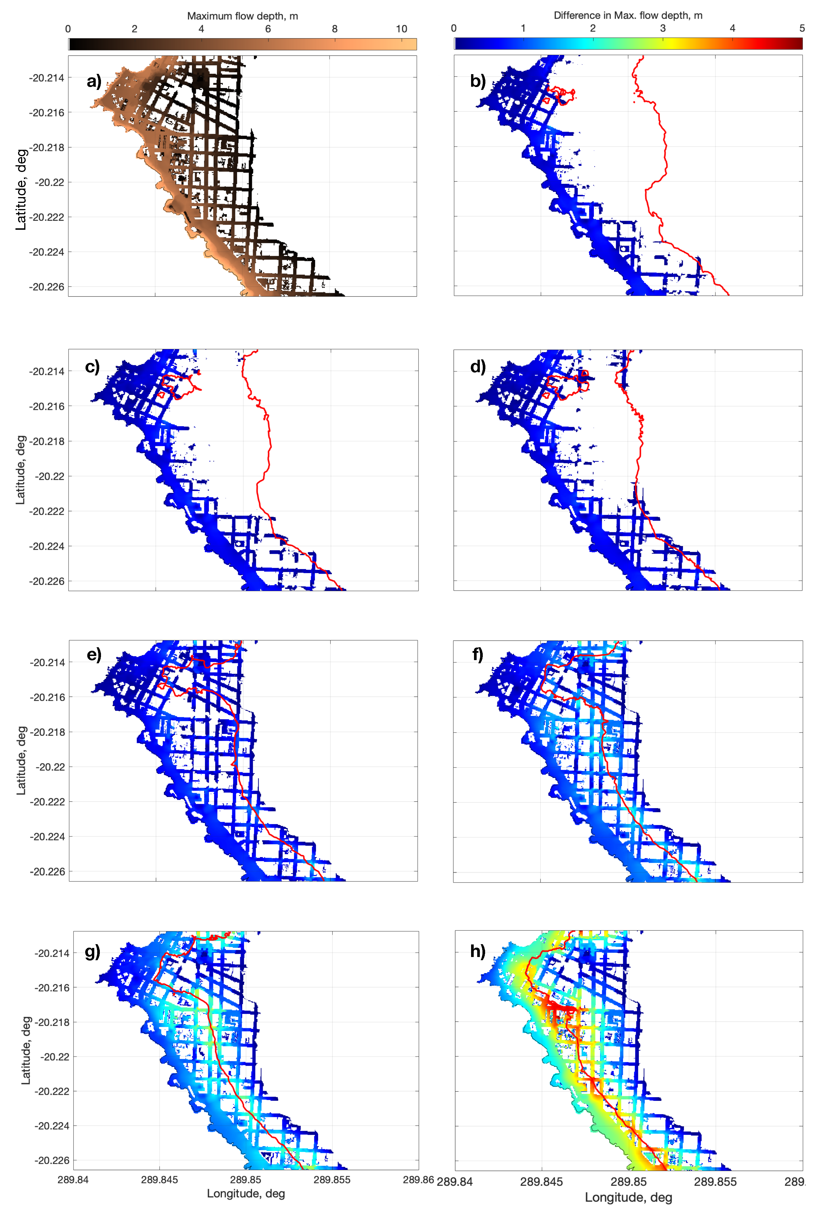
Inundation extent comparison between the DSM model, including resistant buildings, and a DTM model, on Grid-L3b. (a) Inundation extent and maximum flow depth of the reference, DSM model; (b–h) Difference in flow depth extrema between DSM and DTM-CRM, using the maximum grid resolution, . (b) n = 0.025; (c) n = 0.04; (d) n = 0.06; (e) n = 0.10; (f) n = 0.15; (g) n = 0.20; (h) n = 0.40. Red line denotes the inland limit of the maximum inundation of each DTM-CRM model.
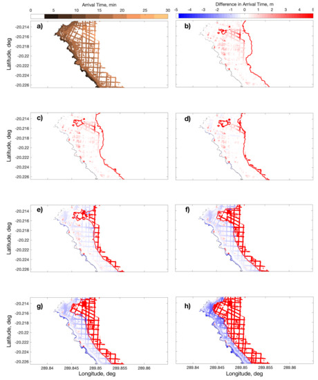
Figure 3.
Arrival time comparison between the DSM model, including resistant buildings, and a DTM model, on Grid-L3b. (a) Arrival time of the reference, DSM model; (b–h) Difference in arrival time between DSM and DTM-CRM, with maximum grid resolution, . (b) n = 0.025; (c) n = 0.04; (d) n = 0.06; (e) n = 0.10; (f) n = 0.15; (g) n = 0.20; (h) n = 0.40. The red line denotes the inland limit of the maximum inundation of each DTM-CRM model.
Figure 2b–h show a comparison between the DSM and DTM-CRM models at the largest resolution. For brevity, sample Manning n values are indicated, which capture the trend in the results. The maps show the difference among extrema
where is the flow depth of the reference model, and is the flow depth of the DTM-CRM model using and grid ratio , , . To simplify the comparisons, the differences are only shown on the streets where the reference value exceeds the DTM-CRM models. The red line denotes the maximum inundation excursion of the corresponding DTM-CRM model. For example, Figure 2b shows that the DTM-CRM using n = 0.025 leads to a relatively small underestimation close to shore, but allows for a much larger inundation area, with depths that are larger than the reference. Figure 2h shows that the inundation area is significantly reduced and that the reference scenario exceeds the maximum flow depths. The DTM-CRM model has thus become too dissipative. The ideal balance can be found when the areal extent is similar and differences are minimal. It appears that 0.06–0.10 offer a good compromise, albeit underestimates the inundated area. These results are consistent with prior research, e.g., [8,11,12,14].
Figure 3a shows the arrival time, as computed by Tsunami-HySEA as the first instance of non-zero flow depth. Figure 3b–h show the differences among these reference values, and those estimated by the DTM-CRM models at maximum resolution
where it is noted that positive differences indicate the reference model arriving later than the DTM-CRM models, indicated by red colors, and the case of no arrival is assumed as having zero arrival time instead of infinity for quantification purposes. The differences in arrival time appear to evolve from early arrivals in the DTM-CRM cases for low Manning n values to delayed arrivals as n increases. It can be noted, however, that differences seldom exceed minutes among the models. 0.04–0.10 yield the best comparison at this model resolution.
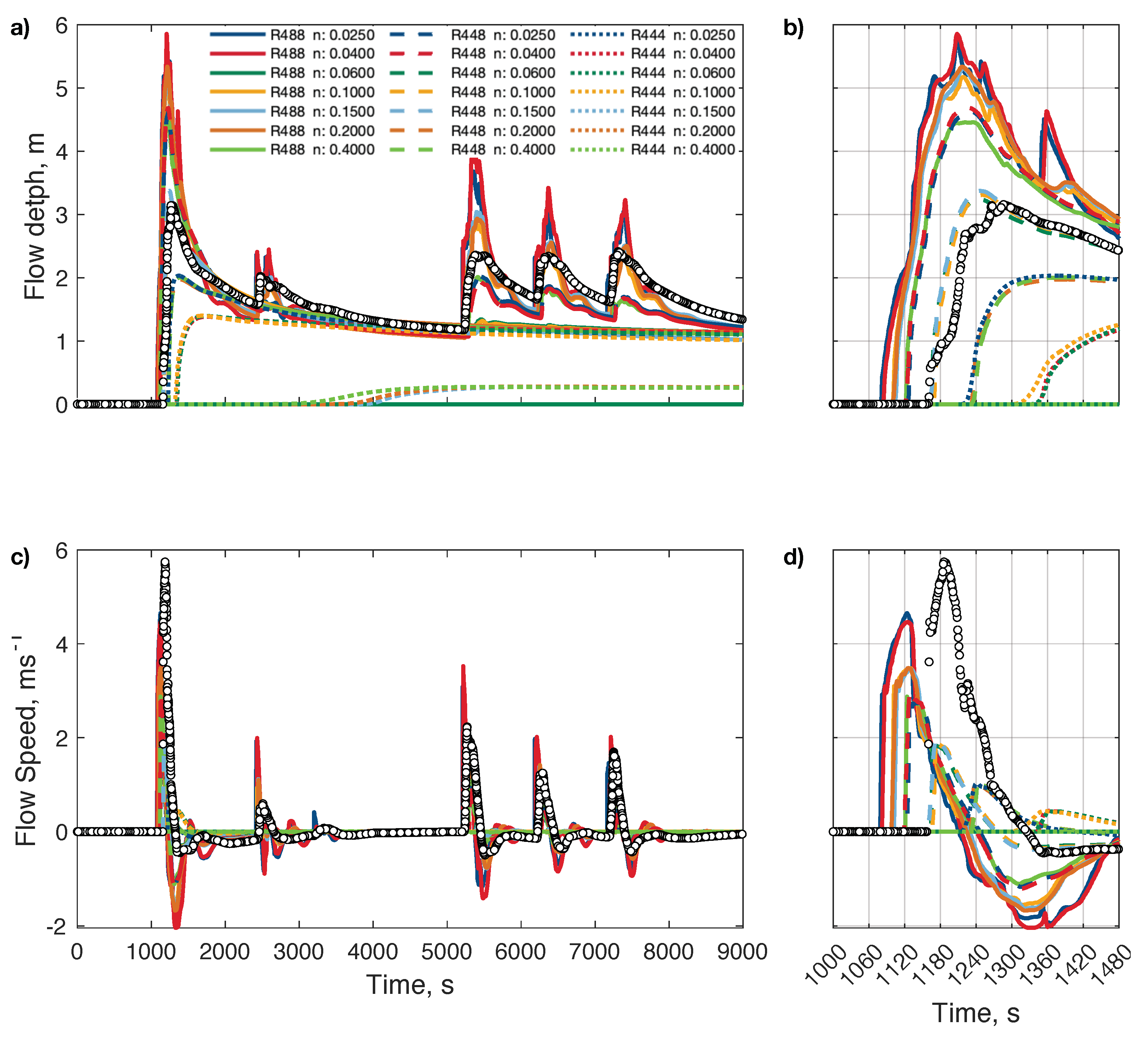
These maps were of integrated TIMs. To explore the effect on the time series, the temporal evolution of flow depth at the inland gauges was considered. A sample comparison using gauge 3 is shown in Figure 4, where all resolutions are shown in different line types, and colors denote different Manning n values. This gauge shows different cycles of inundation, but with very different characteristics as the n value increases. Lower values are characterized by sharp gradients in flow depth and large extrema, coupled with very high velocities. However, for this gauge, none of the DTM-CRM models are capable of reaching the maximum flow speed, which occurs with lower flow depths. The drawdown phase is also characterized by large velocities, which result in a rapid rate of the descent of the inundation. As n is increased, the larger magnitude of the friction force induces less sharp gradients both during inflow and drawdown, the latter with much smaller velocities that lead to a longer flow depth decay. For too large values of n, the attenuation becomes extreme to the point of limiting the occurrence of late arrivals and even affecting the overall structure of the flow, which resembles an almost steady single inundation flow at very low velocities.
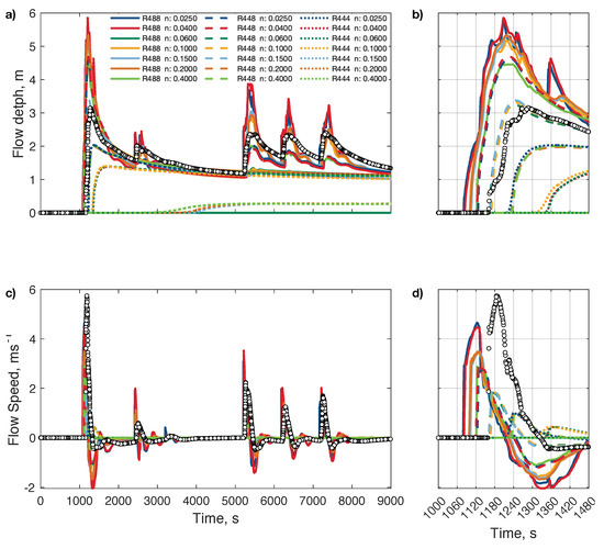
Figure 4.
Time series of flow depth (a,b) and velocity (c,d) at inland gauge 3, for all resolutions (line types) and a range of Manning n values (colors). Circles are the reference model. Panels (b,d) are zoomed in near the first arrival.
To improve the comparison among different Manning n values and resolutions, the difference between the baseline DSM (with n = 0.025 ) and all DTM-CRM models and grid ratios was computed as
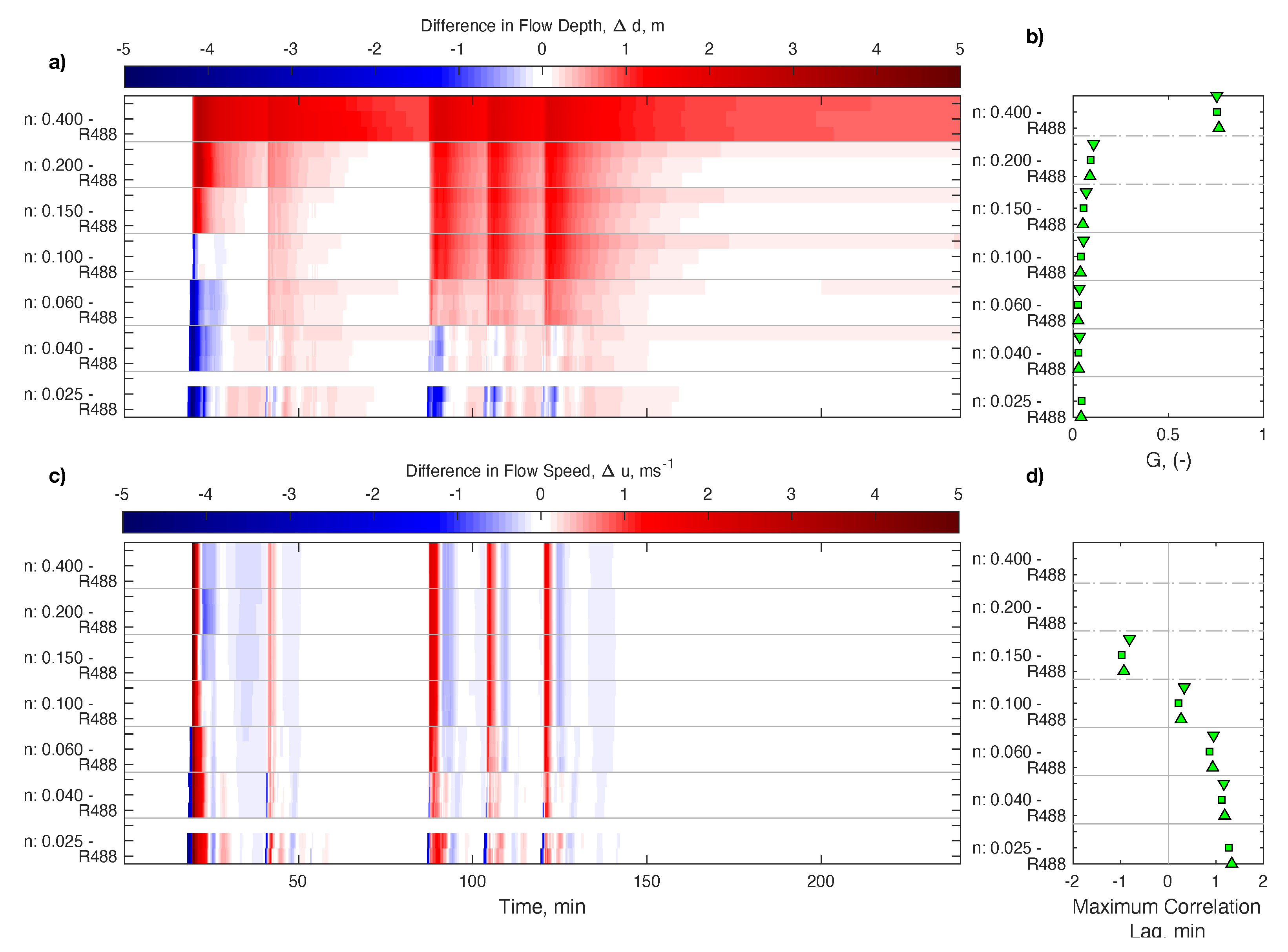
and plotted as maps in Figure 5a,c for the flow depth and velocity, respectively. The ordinate axis is time, and the abscissa is ordered by increasing the Manning n value. For each Manning n value, the three different ratios are presented. Warm colors denote positive , and thus DTM-CRM under prediction. Figure 5a shows that, as the n value increases, there is a transition of the arrival time that gets gradually delayed. However, this effect is relatively small, with maximum differences of approximately two minutes between models. Thus the effect of changing resolutions is small on arrival times. The error in the arrival of the leading wave becomes minimal for . However, matching the arrival time comes at the expense of significantly altering the remainder of the time series. While, for some cases the presence of several waves can be identified, as the Manning n value increases, the modeled flow omits the trailing waves present in the DTM-CRM results, which explains the increase in errors for times exceeding 90 min. Velocity differences follow a similar pattern, but with stronger discrepancies near crests and troughs that are indicative of transitioning from early to late arrivals as the Manning n value increases.
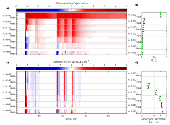
Figure 5.
(a) Comparison of (Equation (6)) for all n values and ratios, for inland gauge 3; (b) Value of the G parameter with (red) and without temporal offset (cyan); (c) Comparison of the velocity error for all n values and ratios; (d) Estimated time lag. In all panels, Manning n values increase vertically, and resolutions decrease vertically for each n value. In panels (b–d), symbols also denote the resolution: ∆, □, ▽.
To summarize these results, different metrics are tested. The bias is omitted because the large number of constant values, many of them zero, will reduce the magnitude of the statistic. Instead, the comparison is made using a normalized least-squares [43,44]:
where denotes the discrete sampling, samples. The formulation without weights was used [44]. G ranges [0,2], with lower values indicating better accuracy. In addition, the cross-correlation between the series was also estimated, along with the time lag that yields maximum correlation. This gives a notion of the offset between models that leads to maximum agreement between the time series. For all metrics, if the time series shows no inundation, it is discarded. Sample results for gauge 3 are shown in Figure 5b–d, respectively. G shows a good overall performance, driven mostly by the good correspondence in the mean inundation level for values of 0.10, where the five inundation cycles are present (see Figure 4a). There is a gradual variation in the G value due to the time offset and the effect of mismatch between instantaneous flow depths, which reaches a minimum between 0.04–0.06. This value departs from our previous analyses that suggested better results for 0.06–0.10, as now the whole time series is considered. Regarding the lags for maximum correlation, the trend confirms the shift between the early arrival of the DTM-CRM series, towards a late arrival as n increases. The optimum is found near .
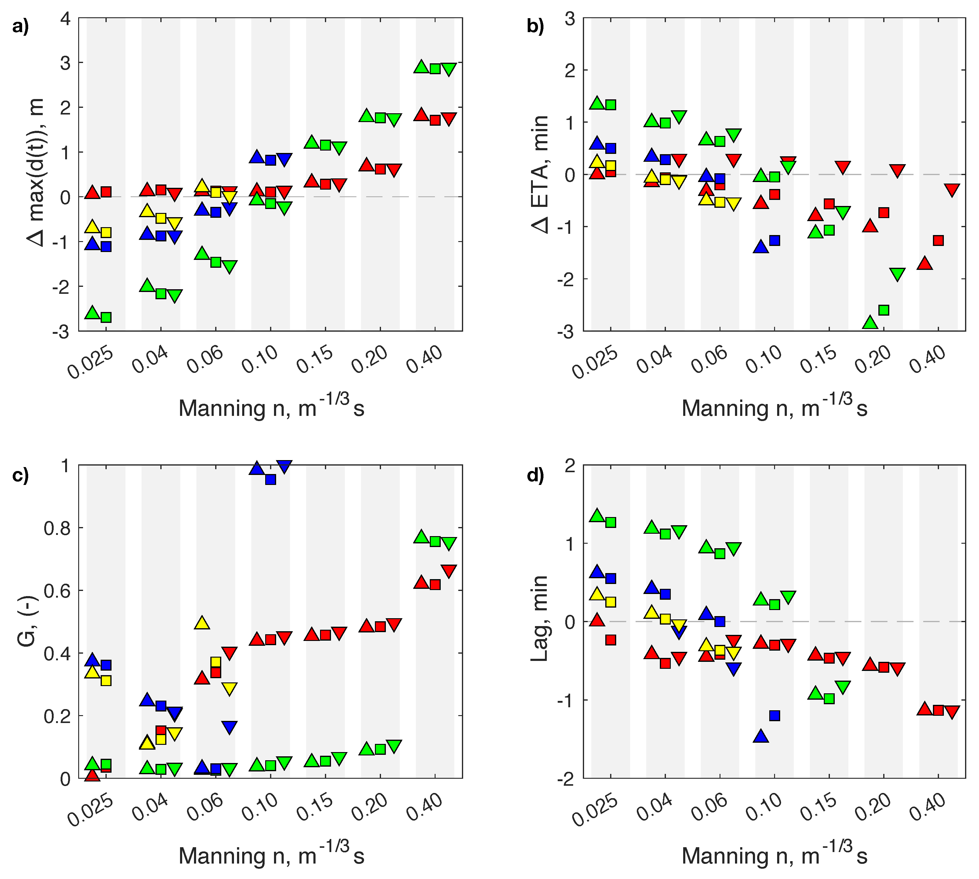
These metrics were computed for all four inland gauges, and aggregated in Figure 6. Panels Figure 6a,b summarize errors in peak flow depth and arrival time. Both errors show linear trends as the Manning n value increases, with similar behavior for all gauges, although the magnitudes vary among them. The flow depth transitions from over-prediction to under-prediction, whereas the arrival time shifts from an early arrival to late arrival. Both metrics appear to reach the smallest error between n = 0.06–0.10 consistently across gauges. For most cases, changing resolutions does not correlate with significant changes in the metrics, especially for smaller n values. The effect is more noticeable for the arrival time than for the error in maximum flow depth, especially for .
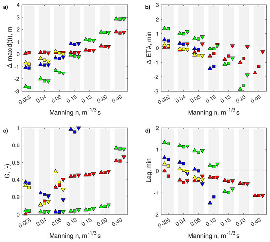
Figure 6.
Summary statistics for all inland gauges, as function of Manning n values. (a) Maximum difference in flow depth; (b) Difference in arrival time; (c) G parameter; and (d) Estimated time lag. Red, green, blue, and yellow markers denote inland gauges 1, 3, 5, and 7, respectively. Symbols also denote the resolution: ∆, □, ▽.
G, in turn, shows a greater sensitivity to the time series characteristics, where no unifying trend can be found. Gauge 5 (blue markers) has the worst performance for , although it did have the best result when n = 0.06. Gauge 7 in yellow shows a similar jump. Both cases are characterized by a single inundation phase. The behaviour is explained in that, as the n value increases, dissipation becomes a dominant term that prevents the flow from reaching that location. The other two gauges show a different behaviour, where performance decreases rapidly as the Manning n value increases. The port gauge 1 (red) is more sensitive to this because the inundation phases are short-lived there. However, as the n value increases, the drawdown phase persists in time, causing a decrease in performance. Gauge 3 does the same, albeit with a smaller sensitivity because, at that location, the drawdown phase is already persistent. For , almost all gauges have , which is considered as a good performance. Finally, time lags follow a similar trend to the arrival time, but with a smaller sensitivity to the grid resolution. Both the error in arrival time and the time lag are generally less than min for .
5. Discussion
The results confirm previous literature in that it is possible to find a suitable Manning n value that reproduces the flow depth and inundation extent of a DSM model, but that velocity fields cannot be reproduced due to the geometrical restrictions that a complex street network and buildings, as modeled by a DSM, impose on the flow. It was found, however, that arrival times are not severely affected by this situation.
This can be explained as follows. The first arrival depends on both the physics and the numerical implementation of the model. The latter refers to the use of a proper algorithm to track dry and wet numerical cells. Here, a single model was tested and no validation data were available; hence, it is not possible to discuss it further. Moreover, the effect of changing the roughness has no direct effect on it.
The main agent that drives the flow is the pressure gradient term. For a cell that has not been inundated before, no prior friction terms exist. Hence, topography and free surface gradients drive the flow into these new cells. Here, and also shown by Yamashita et al. [13], the flow depth profile shows little variation between runs unless the Manning n reaches very large values. This has been suggested to be valid when the topography is gentle [12], as is the case of study here, especially for inland gauge 3. The simulation results share a very steep gradient in flow depth during the first arrival, which could indicate similar values of the force and, therefore, similar flow acceleration. Indeed, lower Manning n values exhibit similar velocity magnitudes and rates of change that confirm this. However, the presence of buildings and the streets network affects the results due to the constriction in the available cross-sectional area for the flow to develop, owing to funneling and blocking. As shown, it is possible to find a Manning n number for DTM-CRM cases in the absence of buildings that imposes enough dissipation to reduce the front flow depth gradient, reducing the forcing and the acceleration enough to mimic the overall behavior of the DSM model, e.g., [45]. However, the dynamics of the flow are not identical. Too large values of the Manning n value have the undesired effect of reducing the free surface gradient, thus forcing too much, leading to slow and gentle inundations that could depart from the baseline model. Whereas, for moderate values, the results show that flow depth time series between the DSM and DTM cases can be similar, the mass flow rate can be significantly different, resulting in strong departures from the reference model in flow velocity.
This behavior was found to be consistent for all inland wave gauges, which share trends in the relevant statistics, even though their flow patterns were dissimilar. Typically, the optimal agreement between baseline and best performing time series occurred for a narrow range of Manning n values, which suggests that, for the differences in geography and urban density explored here, a CRM approach may suffice.
The implications of this are relevant for the modeler. It can thus be argued that no DTM approach could match all the features as modeled by a DSM model. This can lead to costly modeling approaches. However, the modeler could use the Manning n value as a free parameter, thereby departing from the values observed for open channel flow, which can be adjusted depending on the TIM of interest. The results shown herein that the temporal structure of the flow, its extrema, and arrival times are well predicted if a larger value is used, in the range of , which offers a good compromise for most of the metrics tested here. Hence, less computationally costly models at lower grid resolutions could yield similar comparable values to the DSM model that could be used to estimate inundation maps and arrival times of tsunamis. These are useful for evacuation studies, for instance. However, if momentum fluxes and/or flow velocities are considered instead, the error becomes significant both in magnitude and time of occurrence. This may preclude using any of these simplified approaches for the estimation of forces on infrastructure, or fragility curves based on momentum.
It is noted that optimal values for n previously reported based on the inundation extent and flow depth extrema appear to be consistent with the present simulations. Kaiser et al. [8] found a good correspondence when . Present results typically yield an improved performance for n0.06–0.10, although the latter value results already degraded in some of the metrics, such as the G parameter.
For the purpose of arrival time, regarding the quantity of interest for tsunami evacuation that had not been thoroughly analyzed before, the results show to be sensitive to the variation in the Manning n value but confined to ±2 min for the current conditions, while showing a low dependency on the grid resolution. This was the case for both the difference in arrival time and the time lag for maximum cross-correlation. This is significant for expanding tsunami evacuation studies that have typically relied on the more costly DSM modeling. The wall time for the reference DSM model was roughly 220 min, whereas, for the lower resolution DTM-CRM, it was 9 min, on average, with more than a 20× speed up. Considering that it was possible to fine-tune the model configuration to a condition that minimizes all error statistics, this net gain in computing time could be significant to study evacuation planning under a wider range of scenarios.
6. Conclusions
A sensitivity study on the Manning n value’s effect was performed, emphasizing the analysis of the flow’s temporal structure during inundation. Two aspects were considered: the sensitivity of the arrival time and the capability to simulate the overall flow structure by means of different statistics. This was tested in a single domain, and a single, simple earthquake scenario, but this, in principle, should not affect the applicability of the results.
Previous literature was confirmed, in the sense that using a bare land model with an artificially increased value of the roughness can be used to reproduce the inundation extent and maximum flow depths similar to that of a very detailed urban network. However, the range of values that maximize this match can have some significant impact on the temporal structure of the flow, especially if several waves are considered. On the other hand, the arrival time is not overly sensitive to the Manning n value, and it is possible to find a good compromise to speed up calculations, which, in the present case, were accelerated by a factor of roughly 20. On the other hand, velocity time series proved to be more sensitive to the change in geometry between DSM and DTM models, which may preclude the use of the simpler model if velocity-related intensity metrics are of interest.
While the present study did not validate the results against in situ data, the reported values suggest that bare land roughness modeling ought to be increased from the nominal n = 0.025 m to ∼0.06–0.10 m.
Author Contributions
G.C.: Data curation, formal analysis, investigation, methodology, visualization, review, and editing. P.A.C.: Conceptualization, formal analysis, funding acquisition, methodology, investigation, visualization, writing, and supervision. All authors have read and agreed to the published version of the manuscript.
Funding
P.A.C. would like to thank funding by ANID, Chile Grants FONDECYT 1210184, Centro de Investigación para la Gestión Integrada del Riesgo de Desastres (CIGIDEN) ANID/FONDAP/15110017, and Centro Científico Tecnológico de Valparaíso, ANID PIA/APOYO AFB180002.
Data Availability Statement
Bathymetric information was obtained from freely available GEBCO, and upon request from the National and Hydrographic Service of the Chilean Navy, SHOA. http://www.shoa.cl (accessed on 15 January 2022). High resolution topography was obtained from LiDAR flights during the SATREPS Project Research Project on Enhancement of Technology to Develop Tsunami-Resilient Community, 2012–2016, sponsored by the Japan Science and Technology Agency. Data sharing can be considered upon request to the corresponding author. Tsunami HySEA was provided by the EDANYA Research Group of the University of Málaga.
Acknowledgments
We thank Alejandra Gubler and Natalia Zamora for their support in preparing model configurations.
Conflicts of Interest
The authors declare no conflict of interest.
References
- Geist, E.L. Local Tsunamis and Earthquake Source Parameters. Adv. Geophys. 1999, 39, 117–209. [Google Scholar] [CrossRef]
- Mori, N.; Satake, K.; Cox, D.; Goda, K.; Catalán, P.A.; Ho, T.C.; Imamura, F.; Tomiczek, T.; Lynett, P.; Miyashita, T.; et al. Giant tsunami monitoring, early warning and hazard assessment. Nat. Rev. Earth Environ. 2022, 3, 557–572. [Google Scholar] [CrossRef]
- Behrens, J.; Løvholt, F.; Jalayer, F.; Lorito, S.; Salgado-Gálvez, M.A.; Sørensen, M.; Abadie, S.; Aguirre-Ayerbe, I.; Aniel-Quiroga, I.; Babeyko, A.; et al. Probabilistic Tsunami Hazard and Risk Analysis: A Review of Research Gaps. Front. Earth Sci. 2021, 9, 628772. [Google Scholar] [CrossRef]
- Behrens, J.; Dias, F. New Computational Methods in Tsunami Science. Philos. Trans. R. Soc. Lond. Math. Phys. Eng. Sci. 2015, 373, 20140382. [Google Scholar] [CrossRef] [PubMed]
- Imamura, F. Review of Tsunami Simulation with a Finite Difference Method. In Long-Wave Runup Models, Proceedings of the International Workshop; World Scientific: Singapore, 1996; pp. 25–42. [Google Scholar] [CrossRef]
- Bricker, J.D.; Gibson, S.; Takagi, H.; Imamura, F. On the need for larger Manning’s roughness coefficients in depth-integrated tsunami inundation models. Coast. Eng. J. 2015, 57, 1550005. [Google Scholar] [CrossRef]
- Dao, M.H.; Tkalich, P. Tsunami Propagation Modelling: A Sensitivity Study. Nat. Hazards Earth Syst. Sci. 2007, 7, 741–754. [Google Scholar] [CrossRef]
- Kaiser, G.; Scheele, L.; Kortenhaus, A.; Løvholt, F.; Römer, H.; Leschka, S. The Influence of Land Cover Roughness on the Results of High Resolution Tsunami Inundation Modeling. Nat. Hazards Earth Syst. Sci. 2011, 11, 2521–2540. [Google Scholar] [CrossRef]
- Goto, K.; Kawana, T.; Imamura, F. Historical and Geological Evidence of Boulders Deposited by Tsunamis, Southern Ryukyu Islands, Japan. Earth-Sci. Rev. 2010, 102, 77–99. [Google Scholar] [CrossRef]
- Kotani, M.; Imamura, F.; Shuto, N. Tsunami run-up simulation and damage estimation using GIS. Proc. Coast. Eng. JSCE 1998, 45, 356–360. [Google Scholar]
- Gayer, G.; Leschka, S.; Nöhren, I.; Larsen, O.; Günther, H. Tsunami Inundation Modelling Based on Detailed Roughness Maps of Densely Populated Areas. Nat. Hazards Earth Syst. Sci. 2010, 10, 1679–1687. [Google Scholar] [CrossRef]
- Muhari, A.; Imamura, F.; Koshimura, S.; Post, J. Examination of Three Practical Run-up Models for Assessing Tsunami Impact on Highly Populated Areas. Nat. Hazards Earth Syst. Sci. 2011, 11, 3107–3123. [Google Scholar] [CrossRef]
- Yamashita, K.; Suppasri, A.; Oishi, Y.; Imamura, F. Development of a Tsunami Inundation Analysis Model for Urban Areas Using a Porous Body Model. Geosciences 2018, 8, 12. [Google Scholar] [CrossRef]
- Gibbons, S.J.; Lorito, S.; de la Asunción, M.; Volpe, M.; Selva, J.; Macías, J.; Sánchez-Linares, C.; Brizuela, B.; Vöge, M.; Tonini, R.; et al. The Sensitivity of Tsunami Impact to Earthquake Source Parameters and Manning Friction in High-resolution Inundation Simulations. Front. Earth Sci. 2022, 9, 757618. [Google Scholar] [CrossRef]
- Petryk, S.; Bosmajian III, G. Analysis of Flow through Vegetation. J. Hydraul. Div. 1975, 101, 871–884. [Google Scholar] [CrossRef]
- Suppasri, A.; Koshimura, S.; Imamura, F. Developing Tsunami Fragility Curves Based on the Satellite Remote Sensing and the Numerical Modeling of the 2004 Indian Ocean Tsunami in Thailand. Nat. Hazards Earth Syst. Sci. 2011, 11, 173–189. [Google Scholar] [CrossRef]
- Koshimura, S.; Oie, T.; Yanagisawa, H.; Imamura, F. Developing Fragility Functions for Tsunami Damage Estimation Using Numerical Model and Post-tsunami Data from Banda Aceh, Indonesia. Coast. Eng. J. 2009, 51, 243–273. [Google Scholar] [CrossRef]
- Gardi, A.; Valencia, N.; Guillande, R.; André, C. Inventory of Uncertainties Associated with the Process of Tsunami Damage Assessment on Buildings (schema Fp6 Ec Co-funded Project). Nat. Hazards Earth Syst. Sci. 2011, 11, 883–893. [Google Scholar] [CrossRef]
- Tang, L.; Titov, V.V.; Chamberlin, C.D. Development, testing, and applications of site-specific tsunami inundation models for real-time forecasting. J. Geophys. Res. 2009, 114, 12025. [Google Scholar] [CrossRef]
- Härig, S.; Zamora, N.; Gubler, A.; Rakowsky, N. Systematic comparison of tsunami simulations at the Chilean coast based on different numerical approaches. GeoHazards 2022, 3, 345–370. [Google Scholar] [CrossRef]
- León, J.; Catalán, P.A.; Gubler, A. Assessment of Top-down Design of Tsunami Evacuation Strategies Based on Drill and Modelled Data. Front. Earth Sci. 2021, 9, 744193. [Google Scholar] [CrossRef]
- León, J.; Mas, E.; Catalán, P.A.; Moya, L.; Gubler, A.; Koshimura, S.; Cienfuegos, R. Development of calibrated tsunami evacuation models through real-world collected data: The case study of Coquimbo-La Serena, Chile. In IOP Conference Series: Earth and Environmental Science; IOP Publishing: Bristol, UK, 2021; Volume 630. [Google Scholar] [CrossRef]
- León, J.; Castro, S.; Mokrani, C.; Gubler, A. Tsunami evacuation analysis in the urban built environment: A multi-scale perspective through two modeling approaches in Viña del Mar, Chile. Coast. Eng. J. 2020, 62, 389–404. [Google Scholar] [CrossRef]
- Mostafizi, A.; Wang, H.; Cox, D.; Cramer, L.A.; Dong, S. Agent-based tsunami evacuation modeling of unplanned network disruptions for evidence-driven resource allocation and retrofitting strategies. Nat. Hazards 2017, 88, 1347–1372. [Google Scholar] [CrossRef]
- Wang, H.; Mostafizi, A.; Cramer, L.A.; Cox, D.; Park, H. An agent-based model of a multimodal near-field tsunami evacuation: Decision-making and life safety. Transp. Res. Part Emerg. Technol. 2016, 64, 86–100. [Google Scholar] [CrossRef]
- Metois, M.; Socquet, A.; Vigny, C.; Carrizo, D.; Peyrat, S.; Delorme, A.; Maureira, E.; Valderas-Bermejo, M.C.; Ortega, I. Revisiting the North Chile Seismic Gap Segmentation Using GPS-derived Interseismic Coupling. Geophys. J. Int. 2013, 194, 1283–1294. [Google Scholar] [CrossRef]
- Catalán, P.A.; Aránguiz, R.; González, G.; Tomita, T.; Cienfuegos, R.; González, J.; Shrivastava, M.N.; Kumagai, K.; Mokrani, C.; Cortés, P.; et al. The 1 April 2014 Pisagua tsunami: Observations and modeling. Geophys. Res. Lett. 2015, 42, 2918–2925. [Google Scholar] [CrossRef]
- An, C.; Sepúlveda, I.; Liu, P.L.F. Tsunami Source and Its Validation of the 2014 Iquique, Chile Earthquake. Geophys. Res. Lett. 2014, 41, 3988–3994. [Google Scholar] [CrossRef]
- Ruiz, S.; Madariaga, R. Historical and Recent Large Megathrust Earthquakes in Chile. Tectonophysics 2018, 733, 37–56. [Google Scholar] [CrossRef]
- Lomnitz, C. Major Earthquakes of Chile: A Historical Survey, 1535-1960. Seismol. Res. Lett. 2004, 75, 368–378. [Google Scholar] [CrossRef]
- González, J.; González, G.; Aránguiz, R.; Melgar, D.; Zamora, N.; Shrivastava, M.N.; Das, R.; Catalán, P.A.; Cienfuegos, R. A hybrid deterministic and stochastic approach for tsunami hazard assessment in Iquique, Chile. Nat. Hazards 2019, 100, 231–254. [Google Scholar] [CrossRef]
- Cortés, P.; Catalán, P.A.; Aránguiz, R.; Bellotti, G. Tsunami and shelf resonance on the northern Chile coast. J. Geophys. Res. 2017, 122, 7364–7379. [Google Scholar] [CrossRef]
- Simarro, G.; Calvete, D.; Plomaritis, T.A.; Moreno-Noguer, F.; Giannoukakou-Leontsini, I.; Montes, J.; Durán, R. The Influence of Camera Calibration on Nearshore Bathymetry Estimation from UAV Videos. Remote Sens. 2021, 13, 150. [Google Scholar] [CrossRef]
- Cienfuegos, R.; Catalán, P.A.; Urrutia, A.; Benavente, R.; Aránguiz, R.; González, G. What can we do to forecast tsunami hazards in the near field given large epistemic uncertainty in rapid seismic source inversions? Geophys. Res. Lett. 2018, 45, 4944–4955. [Google Scholar] [CrossRef]
- Macías, J.; Castro, M.J.; Escalante, C. Performance assessment of the Tsunami-HySEA model for NTHMP tsunami currents benchmarking. Laboratory Data. Coast. Eng. 2020, 158, 103667. [Google Scholar] [CrossRef]
- Macías, J.; Castro, M.J.; Ortega, S.; Escalante, C.; González-Vida, J.M. Performance Benchmarking of Tsunami-HySEA Model for NTHMP’s Inundation Mapping Activities. Pure Appl. Geophys. 2017, 174, 3147–3183. [Google Scholar] [CrossRef]
- Lynett, P.J.; Gately, K.; Wilson, R.; Montoya, L.; Arcas, D.; Aytore, B.; Bai, Y.; Bricker, J.D.; Castro, M.J.; Cheung, K.F.; et al. Inter-model Analysis of Tsunami-induced Coastal Currents. Ocean Model. 2017, 114, 14–32. [Google Scholar] [CrossRef]
- GEBCO Bathymetric Compilation Group 2019. The GEBCO 2019 Grid-A continuous terrain model of the global oceans and land. Liverp. UK Br. Oceanogr. Data Cent. Natl. Oceanogr. Cent. NERC 2019. [CrossRef]
- Álvarez, G.; Quiroz, M.; León, J.; Cienfuegos, R. Identification and Classification of Urban Micro-vulnerabilities in Tsunami Evacuation Routes for the City of Iquique, Chile. Nat. Hazards Earth Syst. Sci. 2018, 18, 2027–2039. [Google Scholar] [CrossRef]
- Catalán, P.A.; Gubler, A.; Canas, J.C.; Zuniga, C.Z.; Zelaya, C.; Pizarro, L.; Valdes, C.; Mena, R.; Toledo, E.; Cienfuegos, R. Design and Operational Implementation of the Integrated Tsunami Forecast and Warning System in Chile SIPAT. Coast. Eng. J. 2020, 62, 373–388. [Google Scholar] [CrossRef]
- Okada, Y. Surface Deformation Due to Shear and Tensile Faults in a Half-space. Bull. Seismol. Soc. Am. 1985, 75, 1135–1154. [Google Scholar] [CrossRef]
- Aguirre, P.; Vásquez, J.; de la Llera, J.C.; González, J.; González, G. Earthquake Damage Assessment for Deterministic Scenarios in Iquique, Chile. Nat. Hazards 2018, 92, 1433–1461. [Google Scholar] [CrossRef]
- Davies, G. Tsunami Variability from Uncalibrated Stochastic Earthquake Models: Tests against Deep Ocean Observations 2006–2016. Geophys. J. Int. 2019, 218, 1939–1960. [Google Scholar] [CrossRef]
- Romano, F.; Piatanesi, A.; Lorito, S.; Tolomei, C.; Atzori, S.; Murphy, S. Optimal time alignment of tide-gauge tsunami waveforms in nonlinear inversions: Application to the 2015 Illapel (Chile) earthquake. Geophys. Res. Lett. 2016, 43, 11,226–11,235. 2016GL071310. [Google Scholar] [CrossRef]
- Bryson, S.; Epshteyn, Y.; Kurganov, A.; Petrova, G. Well-balanced Positivity Preserving Central-upwind Scheme on Triangular Grids for the Saint-venant System. ESAIM Math. Model. Numer. Anal. 2011, 45, 423–446. [Google Scholar] [CrossRef]
Publisher’s Note: MDPI stays neutral with regard to jurisdictional claims in published maps and institutional affiliations. |
© 2022 by the authors. Licensee MDPI, Basel, Switzerland. This article is an open access article distributed under the terms and conditions of the Creative Commons Attribution (CC BY) license (https://creativecommons.org/licenses/by/4.0/).

