Abstract
Since huge earthquakes are expected along plate subduction zones such as the Japan Trench and Nankai Trough, the estimation of coseismic slip and interseismic slip deficit is essential for immediate response and preliminary measures to reduce damage. Recently, analysis considering the complex topography and underground structure of the plate subduction zone has been performed for improving the estimation performance. However, the three-dimensional (3D) crustal structural model needs to be improved continuously. In this paper, we obtained Green’s functions for 3D crustal structural models with ambiguity by 3D crustal deformation analysis, and the coseismic slip and interseismic slip deficit were estimated. Here we enabled the calculation of many Green’s functions with different physical properties of the 3D crustal structure by utilizing a GPU-based 3D crustal deformation analysis method that significantly reduces the analysis cost. The physical properties on the upper plate’s side, which are located above the plate boundary fault, were changed. We found no significant difference in the estimation performance, except for the upper crust, which most of the fault slip area is in contact with, in the case of coseismic slip estimation. In contrast, the coseismic slip estimation when the properties of the upper crust was changed had a significant error, and a negative slip was estimated at the deep part of the plate boundary where no slip was originally given.
1. Introduction
Many large earthquakes are expected to occur along plate subduction zones, such as Cascadia, Alaska, Chile, Kurill, Japan, and Nankai. When such a large earthquake occurs, the damage is expected to be enormous due to shaking and tsunamis. This damage can be reduced by grasping the phenomenon immediately after the earthquake and providing the immediate and efficient evacuation and emergency response. Important proactive measures can also be implemented, such as considering the rupture scenarios of a massive earthquake before the occurrence, quantitatively assuming the ground motion, crustal deformation and the tsunami caused by those scenarios, and identifying and preparing the vulnerable parts of the city. For the former, estimating the distribution and amount of fault slip is necessary when a large earthquake occurs. For the latter, it is necessary to improve the estimation performances of interplate couplings during the interseismic period. Recently, to improve the estimation performance, analysis using crustal deformation observation data on the seafloor just above the epicenter area of the giant earthquake along the trench is performed [1], and analysis considering the complex topography and underground structure of the plate subduction zone has been performed (e.g., [2]). These results suggest that the effects of realistic topography and subsurface structure cannot be ignored in the slip estimation. Precisely, in the Nankai Trough area, in addition to the on land observation network, an advanced seafloor observation network has been developed [3], and plans for further expansion are underway. Additionally, a three-dimensional (3D) crustal structure model to assume long-period seismic motion has been developed [4,5], and has been used to compute the Green’s function of crustal deformation [6]. However, the crustal structure model needs to be improved in the future, as shown by the fact that the underground structural exploration in the Nankai Trough region has been performed even after the 3D crustal structure model was constructed. In fact, a 3D crustal structure model focused on the offshore has recently been proposed [7]. Therefore, it is essential for the purposes mentioned at the beginning to understand how the model error affects the estimation results quantitatively. However, since the analysis cost of 3D crustal deformation analysis using 3D crustal structure is high, quantitative evaluation of coseismic slip and interplate coupling considering the error of physical properties and the shape of the crustal structure has not been conducted extensively. Few examples have been conducted by our research group, which evaluated the effects of errors on the physical properties and plate boundary shapes on the slip of the Tohoku-oki Earthquake in the Japan Trench area [8,9]. These studies have also shown that ambiguities in the crustal structure model can affect the estimation results, but only a simplified assessment has been made.
Therefore, we have developed a crustal deformation analysis method to perform inverse analysis using a highly detailed 3D crustal structure model, which is essential for the goal of the accurate estimation of highly detailed slip distribution and slip deficit. We integrate GPU-based 3D crustal deformation analysis based on high-performance computation with practical inverse analysis to address more realistic issues which were unexamined in previous studies, such as evaluating which part of the crustal structure mainly affects the estimation slip performance. Specifically, many Green’s functions are obtained by 3D crustal deformation analysis using the proposed 3D crustal structure, and coseismic slip and interseismic slip deficit were estimated considering practical observation errors. Furthermore, many 3D crustal structure models with different physical properties were constructed to consider the ambiguity of the physical properties of the 3D crustal structure, and the effect of ambiguity on the estimation performance of the coseismic slip and the interplate coupling was evaluated. Section 2 shows the 3D crustal deformation analysis and estimation methods of the coseismic slip and interseismic slip deficit, and Section 3 shows the estimation performance evaluated by numerical experiments. Section 4 summarizes the paper.
2. Methods
Herein, we propose an inverse analysis method for evaluating the coseismic slip and interseismic slip deficit on the plate boundary fault using many Green’s functions calculated using a GPU-based 3D crustal deformation analysis method that reduces the analysis cost caused by large-scale 3D crustal deformation analysis. By using the proposed method, we evaluate the estimation performance. The details of the GPU-based 3D crustal deformation analysis method and the inversion analysis method for estimation of the slip and slip deficit are described in this section.
2.1. GPU-Based 3D Crustal Deformation Analysis
Herein, to accurately model the complex crustal structure and accurately consider the stress-free boundary condition at the ground surface, Green’s functions are calculated using the finite element (FE) method with unstructured tetrahedral quadratic elements. Here, the crustal deformation of coseismic slip and interseismic slip deficit due to fault slip is regarded as a linear elastic deformation, and analysis is performed based on the FE method. Using the summation convention, the governing equation is given as:
where,
Here, and f represent the stress and external force. , , , are the first Lame coefficient, strain, Kronecker delta and shear modulus, respectively. By discretizing the governing equation using the FE method, a linear system of equations,
is obtained. Fault slip is evaluated using the split-node technique [10]. Dirichlet boundary conditions are imposed on the bottom and sides of the FE model. Generally, it is difficult to construct a large and accurate 3D FE model that accurately reflects a complex crustal structure. Herein, we used the method reported in Ref. [11] to automatically and robustly generate 3D FE models using unstructured tetrahedral quadratic elements. The mesh around the fault, where localization of deformation is expected to occur, is further refined to generate fine elements without a significant increase in the total FE model size. The computational cost of the FE analysis for large-scale models becomes large. The method reported in Ref. [12] has been proposed for reducing the computational cost of large-scale FE analysis. This method was developed to enable high-speed analysis on CPU based large-scale computing environments. This method was ported to GPU environments using performance portable OpenACC for further enhancing the computational speed. Since the solver is designed to have high parallel performance and reduced memory access, it is possible to demonstrate high performance even on GPU environments. In OpenACC programming, it is possible to port computation to GPU by adding an OpenACC directive clause without making significant changes to the original program. In the operation of the matrix vector product based on the element-by-element (EBE) method [13], it is impossible to allocate temporary arrays for matrix-vector multiplication results considering device memory capacity. Thus, atomic operation is used to add the local matrix-vector multiplication results to a global result vector in EBE kernels on GPUs. Additionally, it has been shown that the performance is sufficiently high even when compared with a program well-tuned by CUDA [14]. For more detailed GPU implementation, see Ref. [15].
2.2. Inverse Analysis of Slip and Slip Deficit on the Plate Boundary
Fault slip is estimated using geodetic data on the ground surface. The slip distribution is expressed as:
where represents the distribution function of the fault slip in the unit fault i, and is the model parameter. The Green’s function, which represents the displacement of the observation point corresponding to each unit fault, is calculated by FE analysis, and the observation model is expressed as:
Here, d represents the observation point data, and H represents the Green’s function. It is assumed that error e follows the normal distribution of the variance-covariance matrix V with a mean value of 0. In addition to the observation errors, e includes errors, such as the uncertainty of the crustal structure model and the high-frequency component of the slip distribution that cannot be expressed by the unit fault. However, we assume that the error corresponding to the observation accuracy independent for each observation point is included in e. Due to the smaller number of observation data compared to the number of unit faults, and errors in the observation data and crust model, inversion may become unstable. To stabilize the inversion problem and obtain a reasonable solution, it is necessary to perform regularization using a priori information on the slip distribution. Here, the model parameters are determined by minimizing the objective function,
where is a term used to constrain the smoothness of the slip distribution [16].
Since it is impossible to assume the area of seismic slip in advance, unit faults are set wider than the area in which the seismic slip actually occurs. As unit faults are defined as a local fault slip, and the actual slip distribution is estimated as a superposition of unit faults, a sparse solution is expected. Therefore, by adding a Group Lasso term to Equation (6), the objective function considering sparsity is expressed as:
Here, g represents a group of variables that correspond to unit faults with different strikes in the same region. This objective function is minimized by alternating direction method of multipliers [17]. As shown later in the results, negative slips appear in some cases for the coseismic slip estimation. Therefore, we also estimated the coseismic slip as the purely opposite direction of the plate convergence by the objective function with non-negative constraints added:
Here, s represents variables for the opposite direction of the plate convergence. For all the above objective functions, hyper parameters of the weight among the terms and are determined by k-fold cross-validation (CV) [18]. Here, the displacement data in all directions measured at one observation point are regarded as one observation data point. In the iteration in CV, the sum of the weighted squared residuals of the validation set and the predicted value based on the slip distribution estimated by the validation set are used as the CV score.
3. Numerical Experiment
Herein, we investigate the estimation performance of the coseismic slip and interseismic slip deficit off the coast of Nankai using the proposed method. Since the Nankai Trough earthquake has not yet occurred since the advanced observation network was installed, we used artificial observation data generated by the virtual coseismic slip based on a large event following Hyodo and Hori [19] (Figure 1). Specifically, a 3D FE model was generated based on the proposed Japan integrated velocity structure model version 1 (JIVSM) [4,5], and artificial observation data were generated by inputting a virtual Nankai Trough coseismic slip and interseismic slip deficit. Here, we used the displacement data at the observation station as the observation data. After adding plausible observation errors to the artificial observation data, we confirmed whether a coseismic slip and interseismic slip deficit could be estimated by inverse analysis [20]. Next, we confirmed the effect of the proposed ambiguity of the physical properties of the crustal structure on the estimation performance.
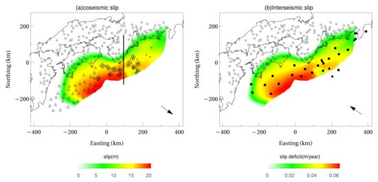
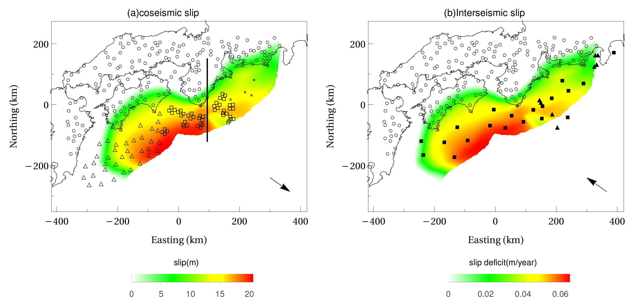
Figure 1.
Reference coseismic slip and interseismic slip deficit distribution. Empty circle, triangle, and squares represent sensors of onshore GNSS, OBP (N-net), and OBP (DONET), respectively. Filled triangle, filled square, and cross represents sensors of GNSS/A (NAGOYA), GNSS/A (JCG), and OBP (JMA) respectively.
First, we explain the 3D FE model. A numerical simulation model for computing Green’s function is constructed based on the JIVSM seismic velocity structure model. The coordinate transformation method of the crustal structure model and the simplification of the layer structure is conducted following Hori et al. [6]. The crustal structure data are projected onto the Cartesian coordinate system with its origin at east longitude , latitude , and the ellipsoidal height 0 m. The target area domain is set between km km, km km, and km . Figure 2 shows the FE model generated by discretizing the target crustal structure model with the minimum element size in the horizontal direction m. From the examination result of Hori et al. [6], an element size of around 500-m is required for numerical convergence of the results; thus, elements are refined such that the element size in the horizontal direction is 500 m in the range of km km, km km, and km km. Here, is the z-coordinate of the plate boundary (for region beyond the trench axis, represent the z-coordinate of the ground surface). The generated FE model comprises tetrahedral quadratic elements with degrees of freedom. The unit fault defined by [6] is used as the basis function. Four hundred and sixty subfaults are set on the plate interface, and two types of unit faults, one in the plate convergence direction and another in the orthogonal direction component, are set respectively. Therefore, it is necessary to compute Green’s functions per crustal structure model. In order to analyze 104 models, including the model of the original physical property values, = 95,680 Green’s functions were computed. Here, a seven compute-node cluster each with a 2.80 GHz 24-core AMD EPYC 7402P CPU and four NVIDIA Tesla A100 GPUs were used in computing the 95,680 Green’s functions (i.e., 28 GPUs were used in parallel with 28 MPI processes). Generally it would require a very large computation cost to compute 95,680 Green’s functions using the FE model with degrees of freedom. However, the analysis time is greatly reduced by using a suitable analysis algorithm and GPU implementation, which allowed for computing all Green’s functions in s (22.0 days).
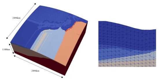
Figure 2.
Generated finite element model. (Left) overview and (right) close up view.
Based on the larger event in the study reported by Hyodo and Hori [19], the virtual Nankai Trough coseismic slip and interseismic slip deficit are set. However, it is moved so that the slip reaches the trench axis, and the slip amount is set to 0 at regions where the unit fault is undefined. The coseismic slip is set to the opposite direction of the plate’s subduction. The reference interseismic slip deficit distribution is set in the opposite direction of the coseismic slip based on Hyodo and Hori [19], with its maximum value scaled to 6.5 cm (Figure 1).
An observation error is added to the calculated observation data based on the assumed error. The observation errors assumed are shown in Table 1. Concerning the observation accuracy, GNSS/A (JCG) is based on the study by Yokota et al. [1], GNSS/A (Nagoya Univ.) is based on the study by Yasuda et al. [21] and Tadokoro et al. [22], DONET real-time is based on the study by Wallace et al. [23], DONET post-processed is based on the study by Machida et al. [24], and others are based on the study by Murakami et al. [20]. The ocean bottom pressure data of N-net under construction from off Shikoku to off Hyuga-nada is also added for the observation data during earthquakes, with the observation error levels set based on the similar S-net system [20]. Observation data with 1000 patterns of independent observation noise is generated for considering the wide variety of observation errors.

Table 1.
Precision of the detection level of the crustal deformation for each sensor in coseismic and interseismic periods.
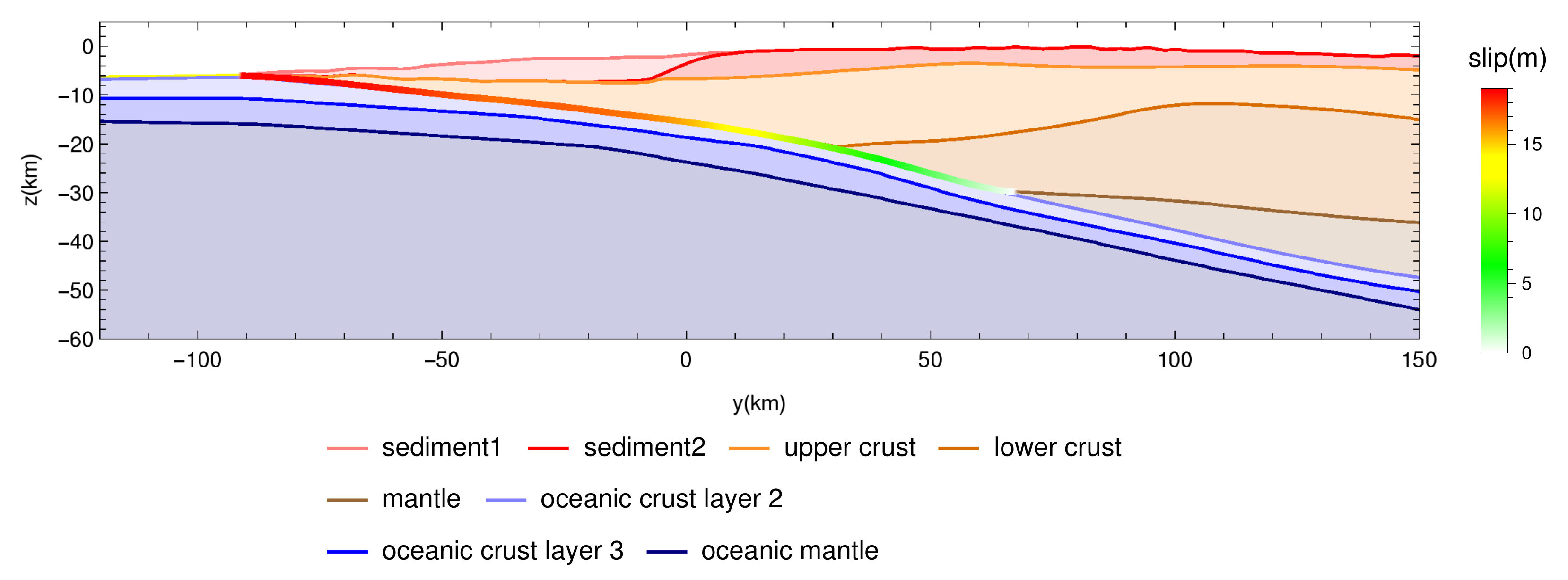
To evaluate the influence of the ambiguity of the crustal structure data to the estimation accuracy, we generated models in which the physical property values of the five layers presented in Table 2 (i.e., sedimentary layer 1, sedimentary layer 2, upper crust, lower crust, and continental mantle) were changed, and the coseismic slip and interseismic slip deficit were estimated based on the computed Green’s function for each model. The range of p wave velocity is set based on JIVSM and the survey results of Nakanishi et al. [7] (Table 2). As the s wave velocity and density follows a linear trend with respect to when similar layers are grouped in JIVSM, we set and from the value of based on the linear regression by the least squares method. Furthermore, the sedimentary layers were grouped into two layers in this model, and a grid search was performed for 100 cases. Regarding the upper crust, lower crust, and continental mantle, the lower limit of the range of assumed physical property values was set as the original physical property values. Three additional cases, where the values of the upper crust, lower crust, and continental mantle were changed to the upper limit value of the assumed property range, were computed. Figure 3 shows the amount of fault slip and the position of each layer in a specific cross-section. Sedimentary layer 1 and upper and lower crusts are distributed just above the fault plane where the large slip occurs in the reference slip distribution; thus, the result of inversion is assumed to be sensitive to the properties of these two layers. It should be noted that most of fault slip area is in contact with the upper crust (Figure 3).
Table 2.
Range of uncertainty in the physical properties of the crustal structure. The lower and upper limits of each property for Sediment correspond to the respective values for layers 1, 8 (Sediment 1) and 7, 14 (Sediment 2) of the JIVSM. The lower limit values for the other layers correspond to the respective values for layers 15, 16, and 17 of the JIVSM. On the other hand, the upper limit values of are the values set as upper limits for the corresponding layers in Nakanishi et al. [7]. For and , linear relationships with the respective values, are estimated from the values of 15, 16, and 17 layers of JIVSM. The relationship with the value of is: and , respectively. For the ambiguity of the sedimentary layers, for sedimentary layers 1 and 2, 10 candidates are set so that they are equally spaced from the range, and 100 physical property values from the combination of these candidates are adopted. In addition, three cases are considered for the upper crust, lower crust, and mantle, each with an upper limit value. Here, the upper limit for the upper crust is larger than the value for the lower crust when given, but this was set to see the effect of the extreme case.
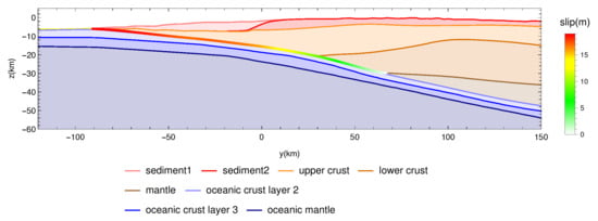
Figure 3.
Cross section of crustal structure along the black line in Figure 1.
3.1. Estimated Result without Ambiguity of Crustal Structure Model
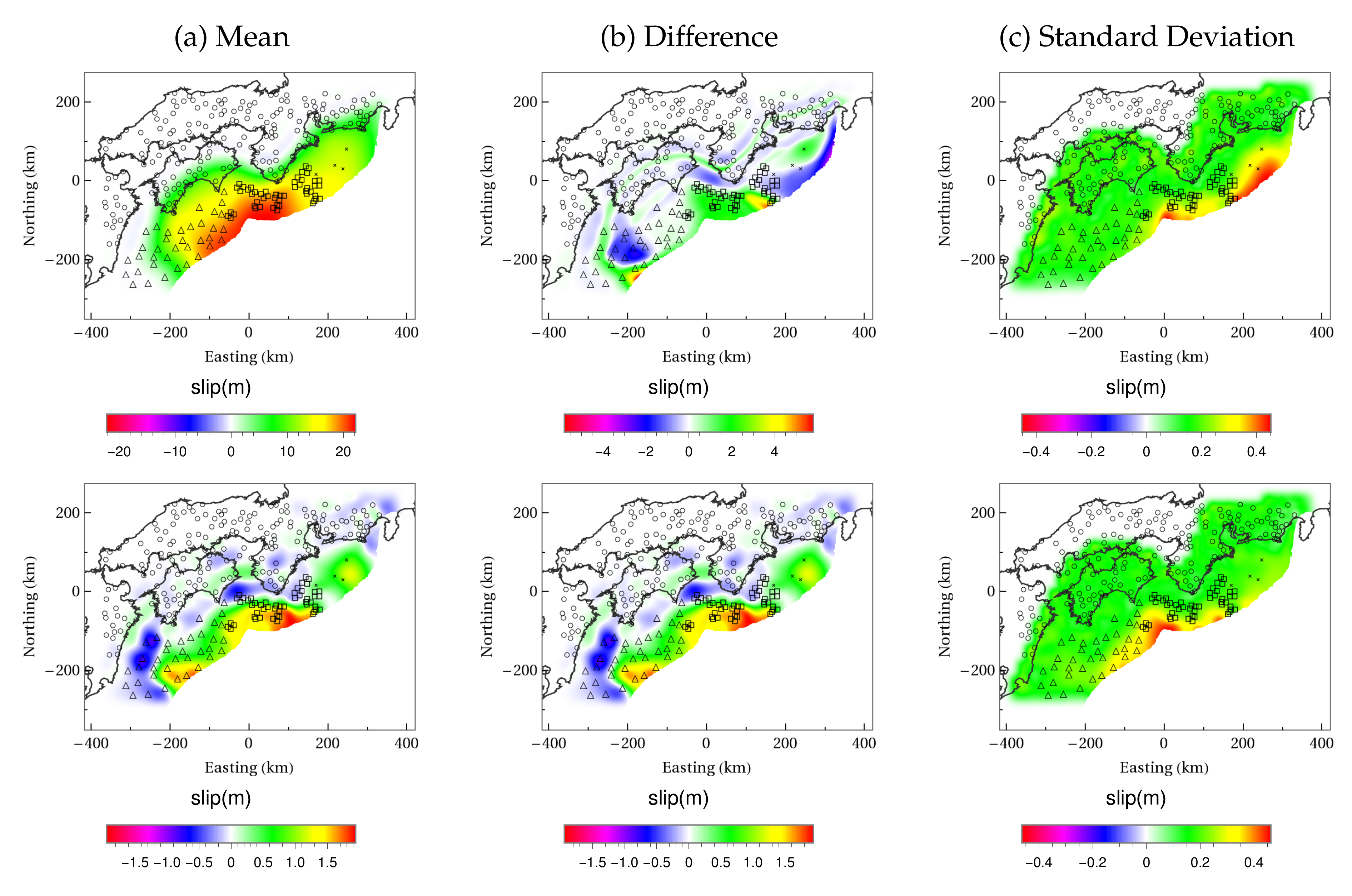
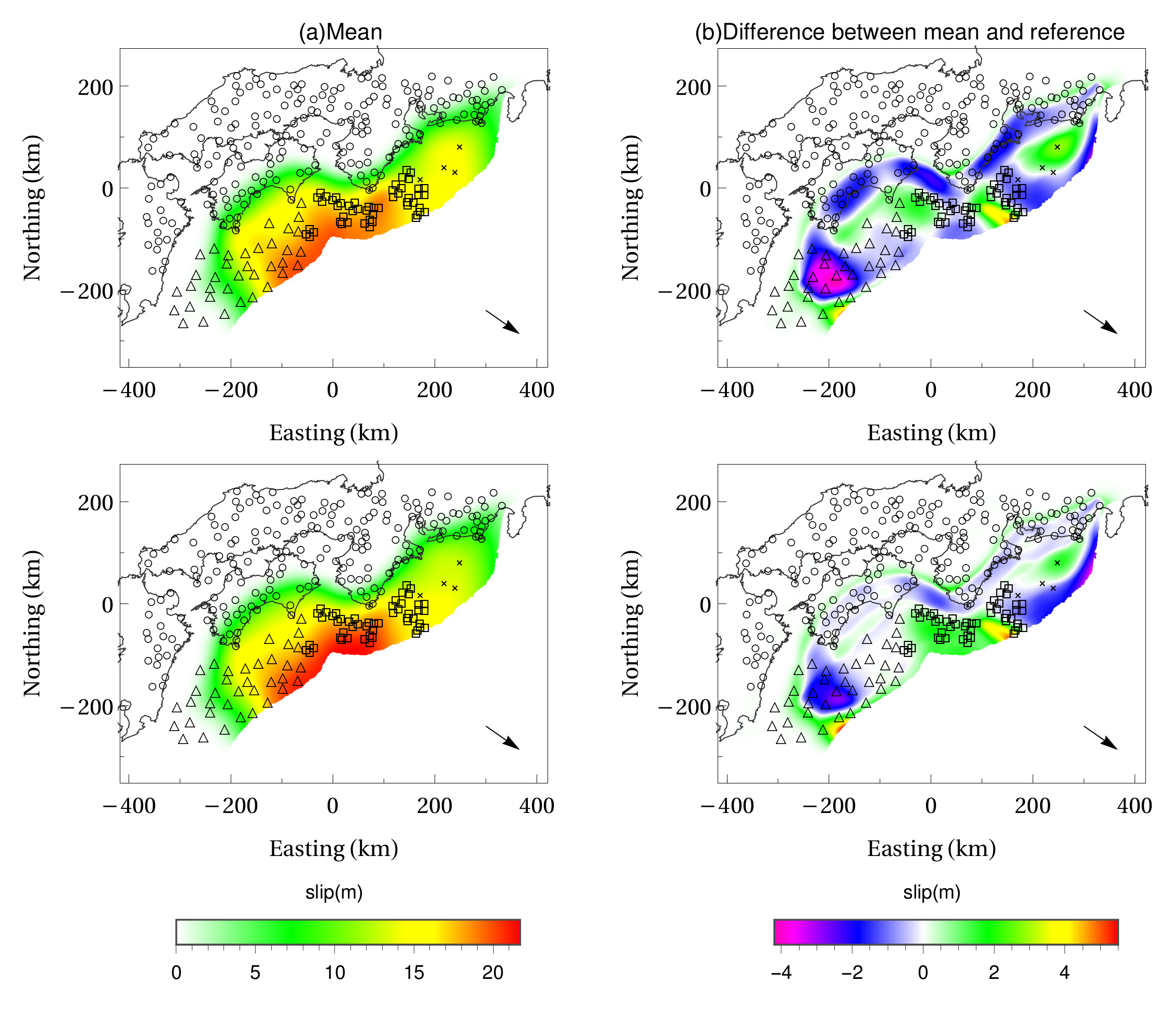
Using the proposed 3D crustal structure model, we evaluated the performance of coseismic slip and interseismic slip deficit estimation. At first we estimated them via optimization expressed in Equation (6). As shown in Figure 4a, the overall behavior could be captured for the coseismic slip. However, the estimation accuracy deteriorates locally far away from the observation point and in places where a steep change is in the reference slip distribution (Figure 4b). The maximum standard deviation is 0.48 m, which is smaller than the maximum slip of 20.58 m and the maximum error of 5.8 m, indicating that the variation in estimation results due to the diversity of measurement errors is small. We can see that regularization suppresses the instability of inversion caused by observation noise. The standard deviation tends to increase in areas where the amount of slip is large, and no observation points exists. In the following, we use the relative error,
as an index of the degree of agreement with the reference slip. While the mean value of relative error for the reference slip was 0.103, the standard deviation of relative error had a very small value of 0.006; thus, we can see that a certain estimation accuracy is obtained regardless of the diversity of the observation errors. Figure 5 shows the ground surface displacement distribution predicted from the mean of the estimated coseismic slip distribution. As horizontal displacement cannot be observed in real-time seafloor observation systems, large differences of 4.30 m and 1.51 m occur in the x and y components of surface displacement at observation points when comparing the cases for the predicted and reference coseismic slip. On the other hand, the maximum error for the z component was 0.12 m; thus, we can see that parameters consistent with observation values were obtained. From the above, we can see that it is difficult to accurately estimate the horizontal component of surface displacement from only the vertical component observations.

Figure 4.
Estimation results in coseismic slip distribution. The mean, difference of mean from reference solution, and standard deviation are shown from left to right for (Above) the opposite direction of the plate convergence and (Bottom) its orthogonal component.

Figure 5.
Surface displacement for estimated coseismic slip. Here, the surface displacement for the reference slip, mean surface displacement for the predicted slip, and its differences are shown for (Above) x component (eastward displacement) and (Below) z component (upward displacement).
Next, the interseismic slip deficit was estimated using the crustal structure model with the original physical property value. Although the observation accuracy is about the same level between real-time and post-processed data, the amount of interseismic slip deficit per year is times smaller than that of the coseismic slip. Therefore, the importance of the observed values in estimating the interseismic slip distribution is relatively smaller, and the geometric mean of the selected was times larger than that of the coseismic case, indicating that the regularization of the spatial smoothing worked more strongly. The mean relative error of the estimated interseismic slip deficit is , which is significantly larger than the estimation error of in the estimation of the coseismic slip distribution. The estimated mean of the interseismic slip-deficit distribution shown in Figure 6 has a smoother distribution, and the error is mainly in the low-frequency components. The standard deviation tends to be large in areas near the trench axis with a large slip.

Figure 6.
Mean value of estimated distribution of slip deficit between earthquakes, difference from reference solution, standard deviation when no ambiguity exists in physical property values. (Above) Plate convergence direction component and (Bottom) its orthogonal component.
3.2. Estimated Result with Ambiguity of Crustal Structure Model
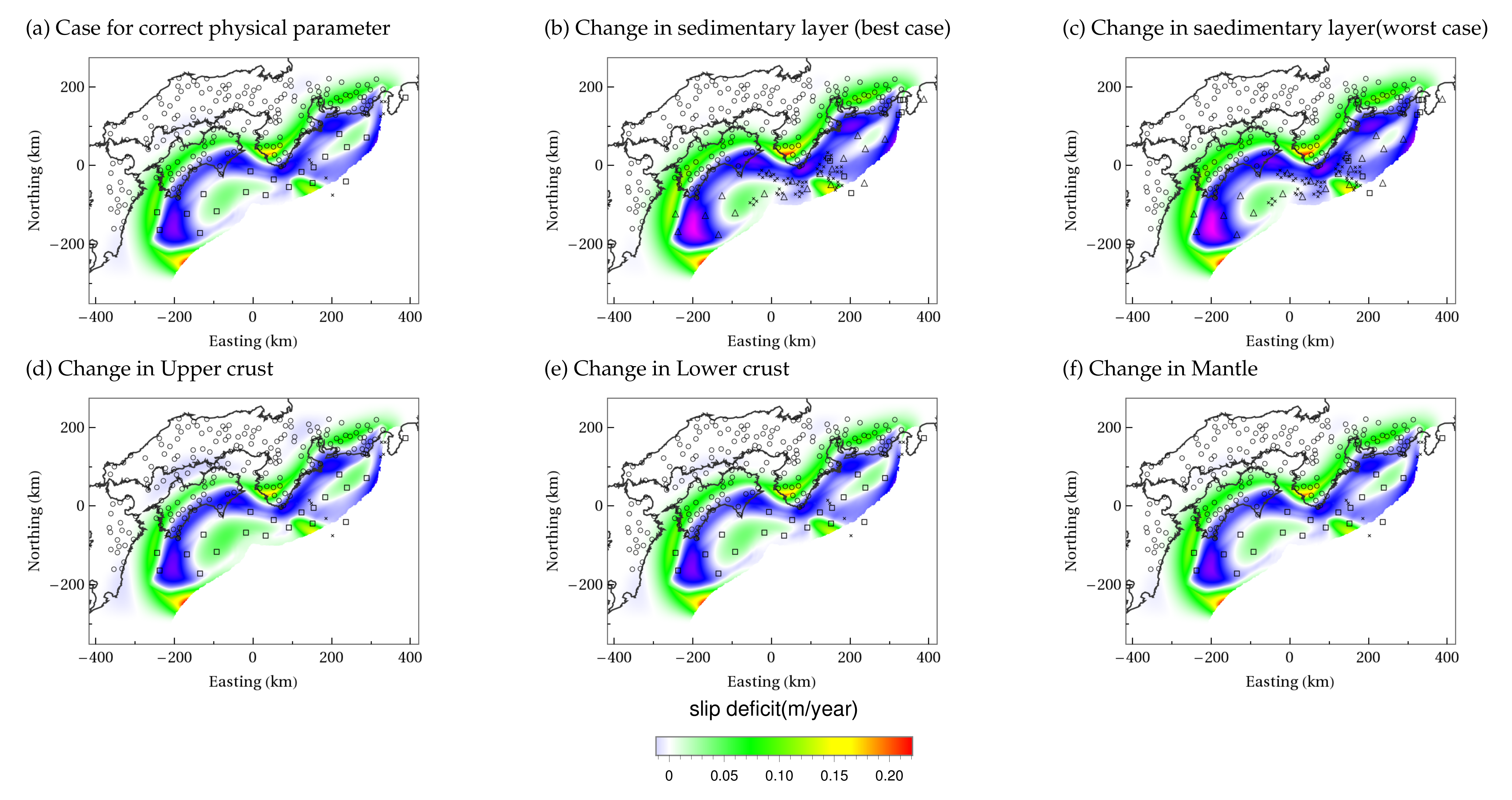
The lowest relative error when changing the properties of the sedimentary layers was 0.097 for m/s, while the largest error was 0.11 for m/s. In the range of considered, the relative error decreased as for sedimentary layer 1 increases, while the relative error was minimized around m/s for sedimentary layer 2 (Figure 7). A similar tendency also exists for the CV score when the optimum hyper parameters are selected, which deviates from the original physical property values (red dot in Figure 7). Therefore, it is impossible to predict the correct physical property values of the sedimentary layer from the estimation results. We can see that the effect of ambiguity of the physical properties of the sedimentary layer on the estimation results of coseismic slip is smaller than the level that can be constrained by the observation data. The relative error when different physical property values were applied to the upper crust increased to 0.127, indicating that the estimation accuracy was significantly reduced. In contrast, estimation accuracy did not change significantly when the physical property values of the lower crust and the continental mantle were changed. Figure 8 shows the plate convergence direction component of estimated slip distribution and the reference solution. In the case of changing the physical property values of the sedimentary layer, there is no remarkable tendency regarding the estimation distribution and estimation error even for the worst parameter case. On the other hand, when the properties of the upper crust are changed, slip in the opposite direction was estimated in a region where slip was zero in the reference solution. In any noise pattern, these negative slips systematically appear only when the physical properties of the upper crust are changed (Figure 9). Additionally, a lower frequency component appears in the difference in the slip distribution in a wide region when the properties of the upper crust are changed (Figure 10). This is due to the inconsistency of the high-frequency components of the Green’s function, which affects the inverse analysis results. In the case where the physical properties of the upper crust is changed, the geometric mean of , which is related to spatial smoothing, is 4.32 times larger than that of the model with correct physical properties; thus, we can see that strong regularization is applied. This trend occurs because it is difficult to reproduce the slip distribution when the noise different from the assumed observation noise (i.e., the error in Green’s functions) is included in the CV. The mean CV score when using the adopted was significantly worse in the case where the physical value of the upper crust was changed to 4880 when compared to the score when using the correct value (2760), which indicates that the observed value is unpredictable due to the error in the Green’s function (Table 3).
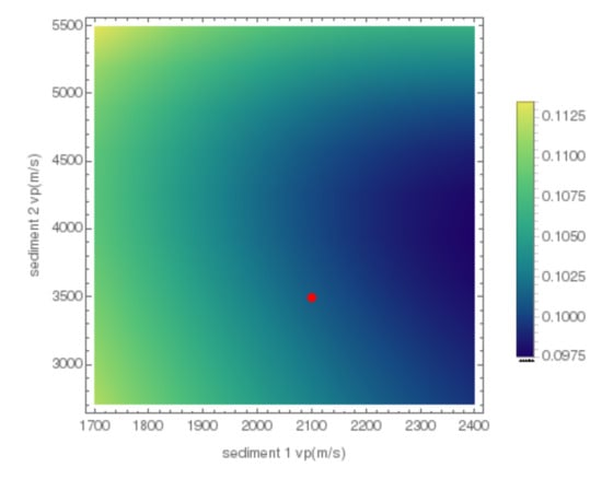
Figure 7.
Average estimation error value when the physical property values of the sedimentary layer are changed. The red dot indicates the physical property values in the reference solution.
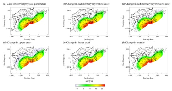
Figure 8.
Estimated coseismic slip distribution (component of opposite direction of the plate convergence) for each case with change in physical properties.
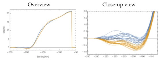
Figure 9.
Cross-section of estimated coseismic slip distribution when no ambiguity exists in the physical properties (blue) and when the physical properties of the upper crust are changed (orange) (line segment between (x, y) = (−50, −185) km and (−250, 115) km). (Left) overview and (right) close-up view of individual estimation results of 20 cases with different observation noise patterns at km km.
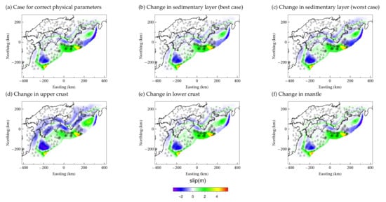
Figure 10.
Difference between the reference and estimated coseismic slip distributions for each case with change in physical properties.
Table 3.
Estimated results for each model. ratio is ratio of to that in case of correct physical property.
Next, we investigated the improvement in the estimation accuracy in estimating coseismic slip when the physical properties of the upper crust, which had a large estimation error, were changed. To suppress the occurrence of slip in the direction opposite to the correct slip direction, estimation was performed by adding a sparse constraint (Equation (7)). Although slip in a part of the seafloor is reduced due to the effect of the Group Lasso constraint, parameters making a sparse estimation was not selected, and the reverse slip remained unsuppressed (Figure 11). We consider the reason is that erroneous estimation of the negative slip does not necessarily reduce the explanation of the observation data when the Green’s functions used are incorrect. In order to confirm our idea, a non-negative constraint condition on the slips in the plate convergence direction component was applied to forcibly obtain a coseismic slip distribution without negative slip, and we examine whether the relative error increases or not. When the model with the original physical property values was used, the negative slip was hardly estimated without non-negative constraints. Therefore, the influence of non-negative constraints should be weak, and actually, the estimated coseismic slip distribution and relative error remain unchanged (Figure 12a). In contrast, when the physical property values of the upper crust were changed, the model parameter in which the negative slip had occurred was suppressed to zero, and the range of slip distribution was more accurately estimated (Figure 12b). However, the relative error increased to 0.142 from the relative error of 0.127 in the case without the non-negative constraints. This confirms that the model error is the reason why the negative slip did not disappear even if the sparse constraint was introduced. From the above, we can assume that the physical properties of the crustal structure model may be set incorrectly if a negative slip is estimated in actual data analysis, as negative slip is not anticipated in an actual coseismic slip. Therefore, we can expect improvement in the estimation accuracy of physical properties by estimating the slip (without non-negative constraints) using Green’s functions of models with varying material properties within the permissible range, and selecting the physical property value that results in non-negative slip.
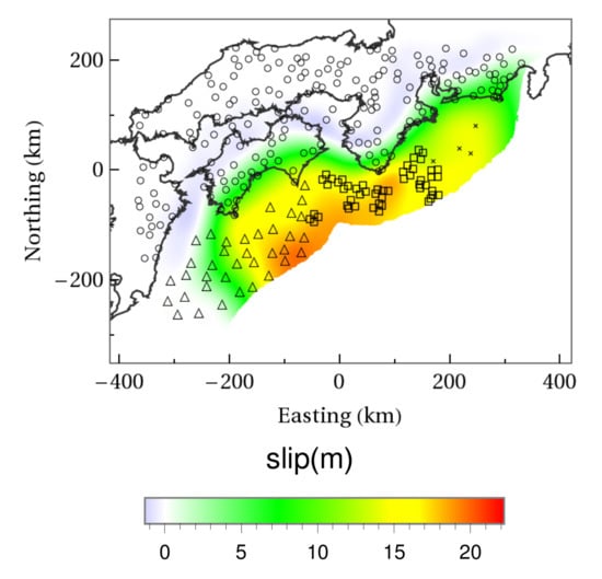
Figure 11.
Estimated coseismic slip distribution under sparse constraints when the physical property values of the upper crust are changed.

Figure 12.
Estimated coseismic slip distribution under non-negative constraints. (Top) Case for correct material properties, and (Bottom) case with change in material properties of upper crust.
In the case of interseismic slip deficit distribution, no significant change was obtained in the relative error when changing the physical properties, even for the case when changing the properties of the sedimentary layer and the upper crust (Table 3). The interseismic slip deficit distribution also shows similar results regardless of changes in the physical property values of any layer (Figure 13). This is expected to be due to the lower S/N ratio in the interseismic observation and effect of regularization, which suppresses the effect of change in the high-frequency component of the Green’s functions.
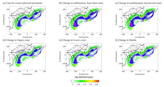
Figure 13.
Difference between the reference and estimated distribution of slip deficit between earthquakes when physical property values are changed.
4. Conclusions
We investigated the effect of the ambiguity of the crustal structure on the estimation performance of the coseimic slip distribution and the interseismic slip-deficit distribution by calculating multiple Green’s functions with different physical property values of the 3D crustal structure by utilizing the GPU-based 3D crustal deformation analysis, which can significantly reduce the analysis cost. Here, we changed the physical property values of the sediment, upper crust, lower crust, and mantle on the upper plate side, which are located above the plate boundary fault that causes coseismic slip and interseismic slip deficit. For the case of interseismic slip deficit estimations, no effects exceeding the observation error levels were found, while for the case of a coseismic slip, no significant difference in estimation performance was obtained except when the physical property values of the upper crust, with which most of the fault slip area is in contact, were changed. However, the estimation of coseismic slip when the physical property values of the upper crust were changed had a large relative error, and the estimation results were systematically biased. Specifically, slip distribution, including components opposite to the direction of the reference slip, was estimated in the deep part of the plate boundary where slip was not originally given. The negative slip is unsuppressed even when using sparse constraints in the estimation, and the relative error became even larger in the case when imposing non-negative constraints to prevent negative slip. From these results, it is suggested that incorrect physical properties are set in the upper crust if a negative slip is estimated using coseismic data, and that a more accurate physical property value of the upper crust can be estimated by finding a physical property value that is unlikely to cause negative slips. While only the observation data of the ground surface displacement is used in this study, the volumetric strain and the inclination change are observed in real-time at several points below the seafloor. Th evaluation of the improvement in the estimation accuracy of coseismic slip and interseimic slip deficits by adding other physical quantities indicating seafloor crustal deformation is our future work.
Author Contributions
T.I. and T.H.; methodology, S.M., T.I and K.F.; software, S.M., T.I and K.F.; validation, T.H. and Y.O.; formal analysis, S.M.; investigation, S.M.; resources, T.I.; data curation, T.H. and Y.O.; writing—original draft preparation, S.M.; writing—review and editing, T.I., K.F., T.H. and Y.O.; visualization, S.M.; supervision, T.I.; project administration, T.I.; funding acquisition, T.I. All authors have read and agreed to the published version of the manuscript.
Funding
This research and APC were supported by the Ministry of Education, Culture, Sports, Science and Technology of Japan (MEXT) as “Program for Promoting Researches on the Supercomputer Fugaku” (Large-scale numerical simulation of earthquake generation, wave propagation and soil amplification: hp200126, hp210171) and by JSPS KAKENHI (JP18H05239). This work was partly supported by MEXT, under its Earthquake and Volcano Hazards Observation and Research Program.
Institutional Review Board Statement
Not applicable.
Informed Consent Statement
Not applicable.
Data Availability Statement
The original contributions presented in the study are included in the article, further inquiries can be directed to the corresponding author.
Acknowledgments
We thank three anonymous reviewers for constructive comments.
Conflicts of Interest
The authors declare no conflict of interest.
References
- Yokota, Y.; Ishikawa, T.; Watanabe, S.I.; Tashiro, T.; Asada, A. Seafloor geodetic constraints on interplate coupling of the Nankai Trough megathrust zone. Nature 2016, 534, 374–377. [Google Scholar] [CrossRef] [PubMed] [Green Version]
- Williams, C.A.; Wallace, L.M. The impact of realistic elastic properties on inversions of shallow subduction interface slow slip events using seafloor geodetic data. Geophys. Res. Lett. 2018, 45, 7462–7470. [Google Scholar] [CrossRef]
- Aoi, S.; Kimura, T.; Ueno, T.; Senna, S.; Azuma, H. Multi-Data Integration System to Capture Detailed Strong Ground Motion in the Tokyo Metropolitan Area. J. Disaster Res. 2021, 16, 684–699. [Google Scholar] [CrossRef]
- Koketsu, K.; Miyake, H.; Afnimar; Tanaka, Y. A proposal for a standard procedure of modeling 3-D velocity structures and its application to the Tokyo metropolitan area, Japan. Tectonophysics 2009, 472, 290–300. [Google Scholar] [CrossRef]
- Koketsu, K.; Miyake, H.; Suzuki, H. Japan integrated velocity structure model version 1. In Proceedings of the 15th World Conference on Earthquake Engineering, Lisbon, Portugal, 24–28 September 2012. Number 1773. [Google Scholar]
- Hori, T.; Agata, R.; Ichimura, T.; Fujita, K.; Yamaguchi, T.; Iinuma, T. High-fidelity elastic Green’s functions for subduction zone models consistent with the global standard geodetic reference system. Earth Planets Space 2021, 73, 41. [Google Scholar] [CrossRef]
- Nakanishi, A.; Takahashi, N.; Yamamoto, Y.; Takahashi, T.; Citak, S.O.; Nakamura, T.; Obana, K.; Kodaira, S.; Kaneda, Y.; Byrne, T.; et al. Three-dimensional plate geometry and P-wave velocity models of the subduction zone in SW Japan: Implications for seismogenesis. Geol. Tectonics Subduction Zones Tribut. Gaku Kimura Geol. Soc. Am. Spec. Pap. 2018, 534, 69–86. [Google Scholar]
- Yamaguchi, T.; Fujita, K.; Ichimura, T.; Hori, T.; Hori, M.; Wijerathne, L. Fast finite element analysis method using multiple GPUs for crustal deformation and its fast finite element analysis method using multiple stochastic inversion analysis with geometry uncertainty. Procedia Comput. Sci. 2017, 108, 765–775. [Google Scholar] [CrossRef]
- Yamaguchi, T.; Ichimura, T.; Yagi, Y.; Agata, R.; Hori, T.; Hori, M. Fast crustal deformation computing method for multiple computations accelerated by a graphics processing unit cluster. Geophys. J. Intenational 2017, 210, 787–800. [Google Scholar] [CrossRef] [Green Version]
- Melosh, H.J.; Raefsky, A. A simple and efficient method for introducing faults into finite element computations. Bull. Seismol. Soc. Am. 1981, 71, 1391–1400. [Google Scholar] [CrossRef]
- Ichimura, T.; Agata, R.; Hori, T.; Hirahara, K.; Hashimoto, C.; Hori, M.; Fukahata, Y. An elastic/viscoelastic finite element analysis method for crustal deformation using a 3-D island-scale high-fidelity model. Geophys. J. Int. 2016, 206, 114–129. [Google Scholar] [CrossRef] [Green Version]
- Fujita, K.; Ichimura, T.; Koyama, K.; Inoue, H.; Hori, M.; Maddegedara, L. Fast and scalable low-order implicit unstructured finite-element solver for Earth’s crust deformation problem. In Proceedings of the Platform for Advanced Scientific Computing Conference, Lugano, Switzerland, 26–28 June 2017; pp. 1–10. [Google Scholar]
- Winget, J.M.; Hughes, T.J.R. Solution algorithms for nonlinear transient heat conduction analysis employing element-by-element iterative strategies. Comput. Methods Appl. Mech. Eng. 1985, 52, 711–815. [Google Scholar] [CrossRef]
- Yamaguchi, T.; Fujita, K.; Ichimura, T.; Naruse, A.; Lalith, M.; Hori, M. GPU implementation of a sophisticated implicit low-order finite element solver with FP21-32-64 computation using OpenACC. In Lecture Notes in Computer Science; Springer: Berlin/Heidelberg, Germany, 2020; pp. 3–24. [Google Scholar]
- Yamaguchi, T.; Fujita, K.; Ichimura, T.; Hori, M.; Lalith, M.; Nakajima, K. Implicit low-order unstructured finite-element multiple simulation enhanced by dense computation using OpenACC. In International Workshop on Accelerator Programming Using Directives; Springer: Berlin/Heidelberg, Germany, 2017; pp. 42–59. [Google Scholar]
- Yabuki, T.; Matsu’ura, M. Geodetic data inversion using a Bayesian information criterion for spatial distribution of fault slip. Geophys. J. Int. 1992, 109, 363–375. [Google Scholar] [CrossRef]
- Glowinski, R.; Marrocco, A. Approximation par -c3-a8l-c3-a8ments finis d’ordre un et r-c3-a8solution par p-c3-a8nalisation-dualit-c3-a8 d’une classe de probl-c3-a9mes non lin-c3-a8aires. R.A.I.R.O. 1975, R2, 41–76. [Google Scholar]
- Blum, A.; Kalai, A.; Langford, J. Beating the hold-out: Bounds for k-fold and progressive cross-validation. In Proceedings of the Twelfth Annual Conference on Computational Learning Theory, Santa Cruz, CA, USA, 7–9 July 1999; pp. 203–208. [Google Scholar]
- Hyodo, M.; Hori, T. Re-examination of possible great interplate earthquake scenarios in the Nankai Trough, southwest Japan, based on recent findings and numerical simulations. Tectonophysics 2013, 600, 175–186. [Google Scholar] [CrossRef]
- Murakami, S.; Ichimura, T.; Fujita, K.; Hori, T.; Ohta, Y. Sensitivity analysis for seafloor geodetic constraints on coseismic slip and interseismic slip-deficit distributions. Front. Earth Sci. 2021, 9, 99. [Google Scholar] [CrossRef]
- Yasuda, K.; Tadokoro, K.; Ikuta, R.; Watanabe, T.; Nagai, S.; Okuda, T.; Fujii, C.; Sayanagi, K. Interplate locking condition derived from seafloor geodetic data at the northernmost part of the Suruga Trough, Japan. Geophys. Res. Lett. 2014, 41, 5806–5812. [Google Scholar] [CrossRef]
- Tadokoro, K.; Kinugasa, N.; Kato, T.; Terada, Y. Experiment of acoustic ranging from GNSS buoy for continuous seafloor crustal deformation measurement. Am. Geophys. Union 2018, 2018, T41Ff-0361. [Google Scholar]
- Wallace, L.M.; Araki, E.; Saffer, D.; Wang, X.; Roesner, A.; Kopf, A.; Nakanishi, A.; Power, W.; Kobayashi, R.; Kinoshita, C.; et al. Near-field observations of an offshore Mw 6.0 earthquake from an integrated seafloor and subseafloor monitoring network at the Nankai Trough, southwest Japan. J. Geophys. Res. Solid Earth 2016, 121, 8338–8351. [Google Scholar] [CrossRef] [Green Version]
- Machida, Y.; Nishida, S.; Kimura, T.; Araki, E. Mobile pressure calibrator for the development of submarine geodetic monitoring systems. J. Geophys. Res. Solid Earth 2020, 125, 125. [Google Scholar] [CrossRef]


Publisher’s Note: MDPI stays neutral with regard to jurisdictional claims in published maps and institutional affiliations. |
© 2022 by the authors. Licensee MDPI, Basel, Switzerland. This article is an open access article distributed under the terms and conditions of the Creative Commons Attribution (CC BY) license (https://creativecommons.org/licenses/by/4.0/).