A Framework for Studying Hydrology-Driven Landslide Hazards in Northwestern US Using Satellite InSAR, Precipitation and Soil Moisture Observations: Early Results and Future Directions

Abstract

The mountainous Pacific Northwest is prone to heavy winter rainfall, resulting in hundreds of landslides per year, human casualties, and billions of dollars of property damage. Precipitation is a major hydrologic trigger for landslides in the northwestern US and around the world. This paper reviews existing literature to outline a framework to study the linkage between precipitation and landslide hazards over the northwestern US using satellite remote sensing techniques including interferometric synthetic aperture radar (InSAR) methods, Tropical Rainfall Measuring Mission (TRMM) satellite precipitation products, and Soil Moisture Active Passive (SMAP) satellite soil moisture data, along with correlation analysis and numerical modeling. InSAR time-series displacements provide an indication of landslide occurrence and extent, and help characterize the basal slip surface and slide-body volume based on the law of mass conservation. Precipitation and soil moisture sensed from the space and ground contribute to creating hydrogeological models associated with water infiltration. These crucial parameters are tracked through correlation and slope stability analysis to understand landslide dynamics. We highlight the results on mapping landslides over the state of Washington and analyses at a few select sites over southern Washington and southwestern Oregon. We conclude that satellite observations of landslide motions and the attributing hydrological variables from both radar and optical images improve our understanding of the inter-relationships between the hydrologic processes along with topographic and geologic settings, and the landslide kinematics and mechanisms inferred from time-series measurements and landslide modeling on a regional scale.

1. Introduction

Landsliding is the downhill movement of soil and/or rock under the force of gravity [1]. This important geomorphic process sculpts the landscapes by transporting large volumes of sediment through the fluvial system [2,3]. Landslide hazards, costing several billions of dollars and resulting in tens of casualties in the United States every year [4], can be triggered by external factors: heavy rainfall or rapid snowmelt [5], ground shaking (volcanic eruptions, earthquakes) [6], changes in land cover (wildfires) [7], atmospheric tides [8], and anthropogenic activities (mining and deforestation) [9] among others.

Dangerous landslides over the northern US have two general categories based on their mobility [10]. One is characterized by long periods of dormancy followed by abrupt mass movements and runout acceleration accompanying the failure of slopes and/or large slump-blocks. A few massive deep-seated landslides (e.g., 2014 Oso landslide in Washington) during lengthened, heavy rainfalls can be extremely mobile and destructive, causing damages and fatalities at a large scale [11,12,13]. The other landslide category exhibits relatively slow motions along a large hillslope, following visco-elastic or visco-plastic behaviors over a long period of time [14,15,16] or coastal marine erosion on the landslide toe [17]. Slow-moving landslides cause significant erosion, regulate hillslope angles and topographic relief, and are a principal geologic hazard to infrastructures [18,19]. In addition, debris flows and mudflows usually occur in small, steep stream channels and are often interpreted as floods. Landslide debris can bulk or add volume and density to otherwise normal stream flow, or cause channel blockages and diversions creating localized erosions or catastrophic flooding. A common trigger for both runout failures and slow-moving landslides is intense precipitation, via an increased pore-water pressure and the attendant reduction in frictional resistance along basal shear zones [20]. Quantifying the interaction between precipitation and landslide initiation and mobility is essential for characterizing the role of landslides in landscape evolution and hazard mitigation [18]. Recurring remote sensing datasets are still facing challenges in identifying and characterizing rapidly-developing shallow landslides and avalanches because the temporal resolution of the data is not frequent enough to capture the dynamic motions of catastrophic landslides which often can exceed the ability of satellite-based remote sensing techniques. However, remote sensing data are better fit to monitoring slowly moving, deep-seated landslides.

The northwestern US is vulnerable to extreme precipitation events (rainfalls of high peaks and long durations) during the winter months. Since 1955, extreme precipitation events have been responsible for about two-thirds of the primary disaster declarations in Washington and Oregon [21]. For example, between December 1996 and Janauary 1997, heavy rainfalls (25–100 cm in two weeks) produced severe flooding over parts of the Washington and Oregon states, causing $3.9 billion in losses and 36 deaths [22]. In January 2009, heavy rainfall and the subsequent flooding closed highways and railways in Washington, and affected major river drainages throughout the northwest. Additionally, the Howard Hanson Dam in Washington was heavily damaged, imposing a great threat to assets and infrastructures, and placing tens of thousands of lives at risk [21,23]. Most major intense precipitation and flooding events in the northwestern US occur with landslides. For example, a devastating runout landslide struck the Oso, Washington in 2014 after a long period of unusually heavy precipitation [11,13].

Monitoring landslide movement constitutes a critical and requisite component of landslide hazard mitigation. However, the traditional investigation and reconnaissance methods over the landslide-prone areas, such as GPS, spirit leveling, tilting, in situ investigation, and optical remote sensing [24,25] cannot alone provide the spatial or temporal resolution required for tracing the landslide development. The interferometric synthetic aperture radar (InSAR) technique has great advantages on broad spatial coverage and high spatio-temporal resolution under all weather conditions (e.g., Refs. [26,27,28,29,30,31,32,33,34]). The InSAR technique has been used in various landslide studies, not only for location detection, but also for deformation monitoring (e.g., Refs. [16,35,36,37,38,39,40,41,42,43,44]). InSAR-derived landslide deformation patterns have provided further insights into landslide dynamics [14,39,41,42,45]. Even though the northwestern US typically has long periods of intense rainfall during the winter season, and is densely vegetated forests, previous studies have demonstrated that longer-wavelength (such as L-band) InSAR techniques are generally capable of penetrating the forest canopy and capturing the concurrent landslide activities through multiple radar acquisitions (e.g., Refs. [13,16,17,18,19,39,42,46]). In addition, recent advances in multi-temporal InSAR processing, such as short baseline subsets (SBAS) InSAR (e.g., Ref. [47]), persistent scatterer InSAR (PSInSAR) (e.g., Refs. [48,49]), and offset tracking techniques [50,51], allow to retrieve time-series deformation by suppressing artifacts related to DEM error, atmospheric artifacts, and other noise.

The widespread network of weather stations, managed by the meteorological agencies (NOAA, local USGS offices) offer real-time and historical precipitation records in and around the landslide regions. However, stations may experience mechanical problems due to heavy rainfall in winter, and many remote landslide sites may be far from the weather stations. Therefore, spaceborne methods, such as Tropical Rainfall Measuring Mission (TRMM) and Global Precipitation Measurement (GPM), can be essential when in situ precipitation measurements are not available [52]. Rainfall intensity and duration, obtained from satellite observations, can be used to infer precipitation thresholds related to incipient landslide motions (e.g., Refs. [12,16,41,46]). Moreover, increased groundwater levels and soil moistures destabilize the slopes through elevated pore-water pressures. This pressure redistribution is a key indicator influencing mass-failure and slope mobility [11]. To overcome the scarcity of measurements that would allow for characterizing these hydrologic parameters in isolated regions of the northwestern US, soil moisture estimates from spaceborne mission—Soil Moisture Active Passive (SMAP)—can be utilized to estimate the groundwater level as well as pore water pressure through a regression model [53].

Simulating a runout event can provide important insights to understand the critical parameters of landslide occurrence [11,12]. Moreover, the simulation before the landslide runout is more critical of managing a future risk as a result of debris flow. Inundation zones based on the best- and worst-case scenarios depending on the mobility of failed materials and basal geometry and thickness of the landslide can be predicted by numerical models [54,55,56]. The outcomes from SAR and InSAR can help derive landslide thickness as crucial inputs for such runout models [57].

The remainder of the paper is constructed as the following. First, we review the satellite-based radar remote sensing techniques in detecting landslide motions and runouts, and in inferring landslide basal geometry based on the InSAR-derived displacement map. Methods on deriving precipitation and soil moisture from the space are briefly introduced. In addition, approaches on studying the correlation between precipitation (soil moisture) and landside movement are described. Second, we review the preliminary results on mapping landslides over the state of Washington from published literature and compare the mapped landslides with existing inventories. Third, we highlight multiple case studies where radar remote sensing and other satellite observations are used to study the dynamics of landslide motions and their causal mechanisms. Fourth, discussions on the limitations of current InSAR techniques and future developments on landslide monitoring are presented.

2. Methodology

2.1. InSAR Methods and Offset Tracking for Mapping Landslide Movements

The use of InSAR for landslide studies has a great advantage compared to other geological survey and other remote sensing technologies. Long frequency of InSAR allows to observe the slope motion beneath forests at high precision of centimeters and spaceborne SAR datasets can cover wide areas (e.g., 70 km swath for ALOS-1/2 stripmap-mode, 350 km swath for Sentinel-1 interferometric wide-swath mode), which help identify landslides over vast regions. Further, a short revisit time of SAR satellites over landslides areas (e.g., 46/14 days for ALOS-1/2 and 12 days for Sentinel-1) can offer temporally dense observations without much added cost for data acquisition, while airborne remote sensing sensors (e.g., LiDAR) are greatly limited by costs and weather condition [58].

If only a limited number of SAR images are available, landslide detection can be done through conventional InSAR based on the phase difference of two or multiple SAR images. However, the conventional InSAR has limitations because the error sources inherent in the outcomes of InSAR (e.g., topographic errors, atmospheric anomalies) cannot be reduced by the use of only a few InSAR pairs. Instead, the errors can be mitigated by utilizing multiple InSAR pairs together. For example, considering the linear relationship between the perpendicular baselines and InSAR unwrapped phases, a regression model from multiple InSAR pairs can be used to reduce the effects of topographic error that are prominent in InSAR results over landslide areas with continuously changing topography. When enough time-series SAR images are available, time-series InSAR mapping of landslide motion can be accomplished through multi-temporal InSAR processing techniques such as PSInSAR and SBAS InSAR (e.g., Refs. [47,48,49,59,60]). Radar targets showing point-like responses characterized by high coherence and phase stability over the entire period of observation are known as persistent scatterers (PSs). Therefore, PSInSAR can provide robust InSAR deformation measurements when sufficient PSs are available. Contrary to a conventional InSAR method, both PSInSAR and SBAS InSAR have the capability of suppressing the errors through regression models and spatiotemporal filtering, and capturing time-series movements at coherent pixels or surfaces over landslides.

Even multi-temporal InSAR technique have limitations. The north-south movements of landslides are insensitive to InSAR acquisitions, because near polar-orbiting SAR satellites are measuring distance from a right angle of satellite moving direction. When landslide motion exceeds InSAR-resolvable displacement or surface condition (vegetation) changes significantly, InSAR methods are not effective. In such cases, offset tracking from multiple SAR images can provide supplementary information regarding landslide motion. Offset tracking through a moving window approach can be used to map landslide motions with an accuracy about 1/20th of the pixel spacings with ideal coherence; the accuracy deteriorates with degrading coherence [30]. Advanced offset tracking methods include the identification of point-like targets prior to the cross-correlation of the image pair (e.g., Refs. [50,51]). As point-like targets resemble 2D sinc-function patterns in SAR amplitude domain, a 2D sinc-function template can be used as a matching template to locate these optimal targets. Then the offset estimation on these point-like targets can be carried out through cross-correlation (e.g., Refs. [50,51]). When both ascending and descending datasets are available, three-dimensional (3D) landslide motions can be obtained through integrating range and azimuth offsets from different satellite trajectories [41]. Although offset tracking has limited accuracy (at ~meter-level) depending on pixel size, correlation, and used window parameters compared to InSAR methods with centimeter-level accuracy, application of offset tracking on multi-temporal SAR images can derive spatio-temporal landslide motions (e.g., Ref. [61]).

2.2. Mapping Landslide Runouts with Digital Elevation Model (DEM), SAR Intensity Images and InSAR Coherence Products

DEMs are required to infer the geometry, volume, and basal slip surface, all of which are necessary inputs for modeling landslide and debris flow dynamics [11]. Numerical analyses of fine scale topography can provide preliminary insights into the geomechanical processes of landslides. The relationship between topographic data and the surface expression of landslide processes can allow the estimation of landslide activity, age, and material type [62,63]. Ideally, the highest resolution DEM (e.g., LiDAR) is needed when modeling landslide dynamics. USGS’s 3DEP and the Puget Sound LiDAR Consortium funded by the NASA, USGS, and local authorities have offered high-resolution LiDAR DEMs over areas in northwestern US. For example, high-resolution DEMs play a key role in evaluating the progress of debris flow in the runout events by inferring the landslide slip-surface, which further allowed the characterization of the landslide mobility and dynamics [11,12]. The 12-m DEM products from TanDEM-X using a bistatic X-band SAR interferometer have been released to only the investigators of approved data proposals, allowing to compile one of the best available DEM datasets for landslide study. However, high-resolution DEMs are not always available over areas with frequent landslides, so we have to rely on alternative, coarser DEMs, such as the previous SRTM DEM and ASTER GDEM. Nevertheless, none of DEMs is perfect for InSAR as the applied SAR data may be operated at different electromagnetic wavelengths, scattered back from different canopy heights, and imaged from different perspectives [42]. Checking and correcting DEM errors are necessary for InSAR applications on hilly, forested landscapes, in particular for interferograms with large spatial baselines.

SAR intensity images are sensitive to terrain slope, surface roughness, and target dielectric constant, and therefore can be used to map landscape changes caused by landslide runouts. As SAR backscattering returns can be affected by speckle noise, time-series analysis of multi-temporal SAR intensity images is especially useful to detect landslide runouts of different scales (e.g., Ref. [42]). As landslide runouts are often accompanied by inclement weather conditions, all-weather SAR intensity imagery can be the most useful data source available to track the runout events.

InSAR coherence map, a cross-correlation product derived from two co-registered SAR images, can depict changes in backscattering characteristics on the scale of radar wavelength. Over landslide-prone regions, loss of InSAR coherence (i.e., decorrelation) renders an InSAR image useless for measuring landslide motions. However, the patterns of InSAR coherence loss can provide clues on surface modifications caused by landslide runouts and other environmental factors.

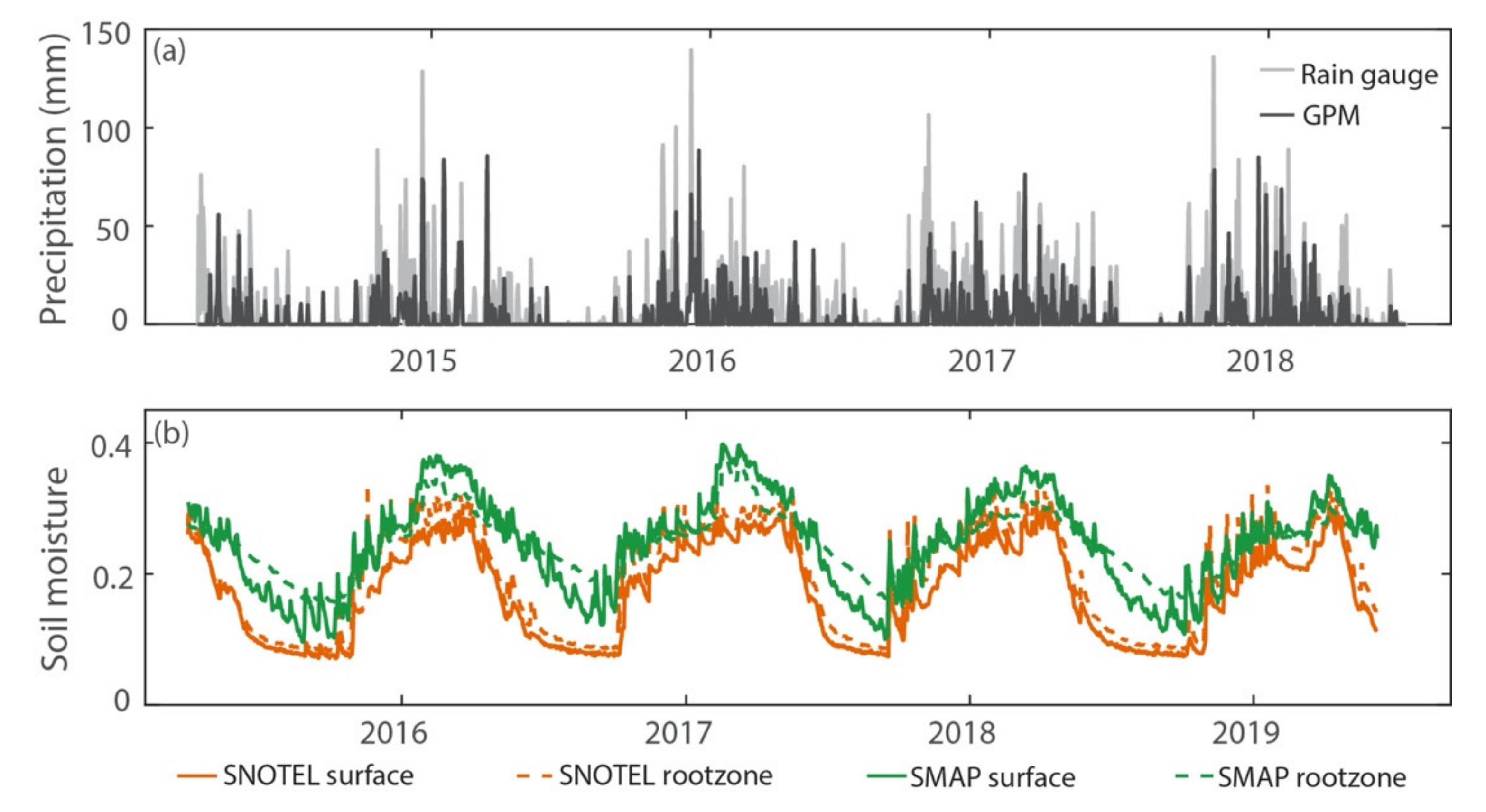
2.3. Precipitation Observations from Space and Ground

Past studies have recognized the strong correlation between the landslide motions estimated from InSAR methods and the precipitation in the northwestern US (e.g., [13,16,42,46]). However, precipitation measurements from in situ stations are often sparse. Hence, the satellite-derived precipitation can be essential in the correlation analysis, when the landslides, in many cases, occur in isolated mountainous areas and the precipitation at weather stations during heavy rainfall is often missing. The TRMM-based Multi-satellite Precipitation Analysis (TMPA) provides an opportunity to evaluate how rainfall attributes affect the spatial distribution and timing of landslides in regions that suffer from lack of weather stations. TMPA provides a calibration-based sequential scheme for combining precipitation estimates from multiple satellites, as well as gauge analyses where feasible, at fine scales (0.25° × 0.25° 3-hourly) over the latitude band 50° N-S (http://trmm.gsfc.nasa.gov accessed on 21 April 2021). The TMPA is a TRMM standard product computed for the entire TRMM period (January 1998 to April 2015). The GPM is the follow-on mission of TRMM, which is a joint satellite project between NASA and JAXA, providing a product similar to its predecessor. With real-time measurements, a post-processed product incorporating gauge data at the present with 3-hourly satellite estimates can be used for long-term monitoring of landslides (e.g., Ref. [64]).

2.4. Soil Moisture Measurements Using SMAP

Following heavy rainfall and with an elevated groundwater level, the rising moisture in surface and subsurface layers can increase the basal pore water pressures, and influence the mobility and eventual runout of the landslide. The soil moisture is one of key parameters to understand the landslide dynamics at regional and global scales. In the northwestern US, in situ gauges to measure soil moisture are sparsely installed and managed. The limited collection of soil moisture in landslide-prone mountainous region restricts the susceptibility assessment and landslide early warning. The Soil Moisture and Ocean Salinity (SMOS) and Advanced Microwave Scanning Radiometer (AMSR-E) have successfully delivered soil moisture data. The SMAP launched in January 2015 can provide the global soil moisture measurements. NASA’s SMAP mission planned to use L-band SAR and radiometer to estimate concurrent, coincident soil moisture integrated as a single observation system, and the combination of active (SAR) and passive (radiometer) sensors could synergistically improve resolution and sensitivity to soil moisture, surface roughness, and vegetation scattering [65]. Although the active SAR sensor ended operations due to a power failure after July 2015, the SMAP’s radiometer-derived and science value-added products still offer a unique opportunity to measure soil moisture (particularly in the top 5 cm of the soil column) over steep terrain in the northwest from the space. The SMAP Level 4 soil moisture products are achieved through assimilating a land surface model that monitors the evolution of soil moisture, snow, temperature, and precipitation [65]. The nominal resolution of Level 4 SMAP surface soil moisture (unit: m³/m³) data is about 9 km.

A recent study has found a close relationship over the vegetated areas among SMAP-sensed soil moisture, groundwater level, and precipitation [66]. As soil moisture is a better indicator gauging the onset of landslide motions [67], soil moisture can be better suited to study the correlation between precipitation and landslide motion.

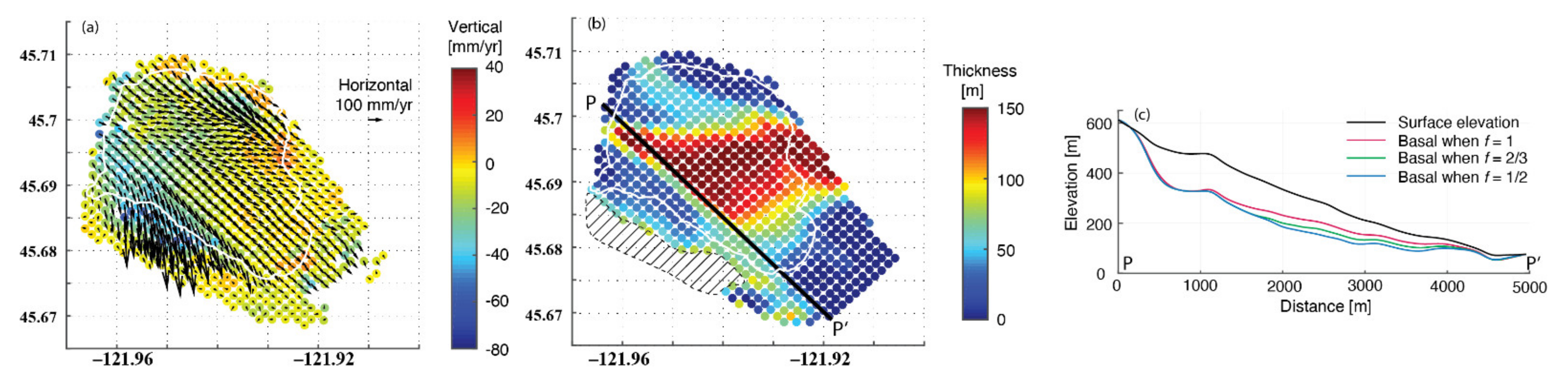
2.5. Landslide Basal Geometry and Volume from Inversion of InSAR Displacement

Estimating landslide thickness is important for assessing landslide hazards, because thickness is closely related to the volume of landslides as a result of failed slope that can lead to a longer runout distance with highly mobile materials and low friction of basal surface. The surface deformation measurements from InSAR allow possibilities of inverting for the depth and orientation of the basal plane. There are at least two approaches of estimating landslide thickness on the basis of surface deformation. One is to model the landslide as a feature of faulting using elastic models [68]; this approach is applicable to rockslides (e.g., [69,70,71]). The other method originated from the glacier ice community is to use the conservation of mass and a free surface kinematic boundary condition [46,71,72] (Figure 1):

$$w=-f\nabla \cdot (h{V}_{hor})$$

(1)

where w is the surface vertical rate (derivative of elevation with time), and V_hor is the two-dimensional surface horizontal velocity vector, f is a rheology parameter ranging from 0 to 1, and h is landslide thickness ([71]; Figure 1). This model can be further simplified by assuming that the rheological condition of the landslide body is spatially uniform, so f is a constant and equals to 1 − Y/(3h), where Y is the thickness of the yield zone and h is the landslide thickness (Figure 1). In a general case of power-law rheology, f = 1/2 corresponds to a linear vertical velocity profile, f = 2/3 to Newtonian viscous flow when the entire depth has yielded and the plug region vanishes, and f = 1 to a rigid sliding block when the yield zone vanishes [46,71]. When less than three distinct perspectives on motion estimates are available, it is often assumed that the landslide slips along the largest topographic gradient on the slope-parallel plane, which helps constrain the 3D displacements from ascending and descending InSAR results (e.g., [46]). Equation (1) can be discretized on a regular grid using finite difference approximations in matrix form, and resolved by the non-negative least-squares method [46,71].

2.6. Understanding the Delay between Landslide Movement and Precipitation—Pore-Water Pressure Diffusion Modeling

Precipitation, subsequent infiltration, and elevated pore-water pressure can result in landslide movement [5]. To find the linkage between rainfall and slope destabilization, the precipitation record can be used to establish a simple 1-dimensional (1D) pore-water pressure diffusion model [5,73,74,75,76]:

$$\frac{dp}{dt}=\alpha \frac{d^{2}p}{d{z}^2}$$

(2)

where the pore-water pressure p is a function of depth z and time t, α represents the effective hydraulic diffusivity. The pore-water pressure at the ground surface can be approximated as cW(t), where W(t) is the precipitation record and c is a scaling factor modulating the amplitude of pore-water pressure changes. Then, the solution of 1D pore-water pressure diffusion equation can be given as:

$$p\left(t,z\right)=\frac{cz}{2\sqrt{\pi \alpha }}{\displaystyle {\int }_0^t\frac{e^{\frac{-z^2}{4\alpha (t-\tau )}}}{\sqrt{{\left(t-\tau \right)}^3}}}W\left(\tau \right)d\tau$$

(3)

The pore-water pressure can be solved via Fourier transforms [73,74,75,76] to obtain hydraulic diffusivity and study the correlation (and time lag) between the observed landslide movement time-series and precipitation record.

2.7. Landslide Runout Simulation

Researchers have routinely developed and applied depth-averaged mathematical models for simulating landslide and debris-flow dynamics. Physics-based models should not neglect solid-fluid effects that control the macroscopic rheological behavior of granular-fluid flows. The open-source D-Claw model is a two-phase granular-fluid model that can model landslides and debris flows, from initiation to deposition [11,12]. This model has been successfully validated with extensive comparisons with large-scale experimental data from the USGS debris-flow flume, and has been validated with post-event data from naturally occurring events, such as the 2014 Oso landslide [11,12,77]. With this model, landslide motion is instigated when a statically balanced initial state is perturbed by gradually rising basal pore-fluid pressure. The model parameters are all based on theoretically measurable material properties of hydrologic and sediment material properties. Additionally, the model’s requisite initial conditions include potential failure volumes and geometries. While the physical dependencies of landslide stability, mobility, and dynamics on these model parameters are largely understood theoretically, constraining these parameters in practice can be difficult. Parameter and geomechanical information, derived from multi-temporal InSAR methods, provides constraints on initial conditions and model material parameters that influence landslide susceptibility and mobility. In terms of sensitivities, soil porosity, permeability, and interstitial pore–fluid pressures play a dominant role in landslide mobility given incipient motion. Remotely sensed precipitation and soil moistures can be used to estimate the variation of pore-water pressure with supplementary knowledge on soil compaction, density, porosity, fluid viscosity, and permeability.

3. Early Results

The Pacific Northwest extends over 800 km from Washington to Oregon to northern California. The oceanic Juan de Fuca plate in the west of the region is subducting below the North American continental plate along the Cascadia subduction zone. Pacific Northwest can be divided into eastern and western area by the Cascade Range, and each has different climates due to differences in rainfall and temperature. Contrary to eastern region with less precipitation in most places, the western Pacific Northwest receives much more rainfalls and the precipitation in some places of the Coast Range exceeds 2 m per year [78]. Inland Cascade Range creates steep terrain to the west of Cascadia coastline and the Pacific Northwest is underlain by Laurentia (pre-Jurassic rocks indegenous to ancestral North America), terranes that accreted to Laurentia in the past 185 million years by plate tectonic processes, and sedimentary and volcanic rocks less than 56 million years old. Because of the steep terrain and high precipitation in winter, landslides are common in the western Pacific Northwest and most landslide studies have focused on the landslides in the area [78,79].

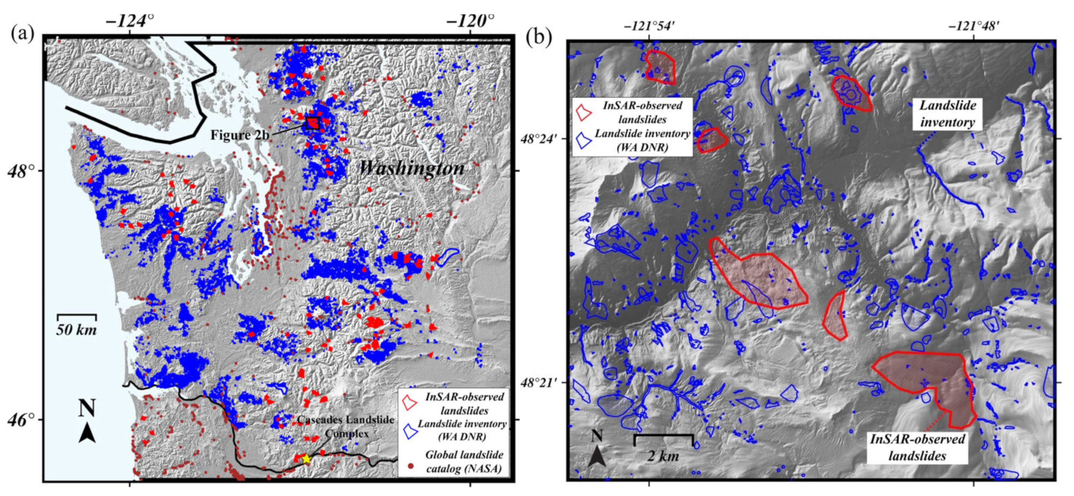
3.1. Updating Landslide Inventory with InSAR

The landslide inventory map plays a critical role in assessing the landslide hazards and evaluating the slope stability from their spatial distribution [80]. The state and federal agencies have distributed the landslide inventory maps developed from geological maps, topography, and historical landslide events. Washington Department of Natural Resources (DNR) provides the inventory map from Washington Geologic Information Portal (https://geologyportal.dnr.wa.gov accessed on 21 April 2021). The statewide landslide inventory provides information about landslide type (e.g., deep-seated landslide, debris slide, avalanches), slope morphology, location confidence/certainty, etc. NASA landslide viewer (https://landslides.nasa.gov/viewer accessed on 21 April 2021) as a part of federal program collected the world-wide landslides based on reporting of governments and civilians.

The state of Washington is prone to frequent, seasonally recurring landslides, because the region with steep terrain experiences extreme precipitation events during the winter months and the hydrologic force triggers the deep-seated landslides. While the landslides in Washington caused the fatalities and costed billions of dollars in property damage (e.g., 2014 Oso mudslide that resulted in 43 fatalities), a close correlation between landslides and intense precipitation is obvious. However, the locations, dimensions, geographical extent, and activeness of the landslides in the Washington are not well known. Therefore, mapping landsides over the region is essential for hazard mitigation, risk assessment, and characterization of each landslide.

ALOS-2 PALSAR-2 InSAR pairs with short perpendicular baselines give the best opportunity to locate the landslide hazards in Washington and delineate their extents. One drawback of ALOS-2 PALSAR-2 is its sparse acquisitions in the region. Despite 14 days of revisit days, only 4~6 images a year from the same track are available for most of the state of Washington, which prevents the generation of dense time-series deformation. However, most interferograms from different seasons within a year (i.e., winter to summer) or between summers of different years with short perpendicular baselines (<100 m) maintain coherence in forested areas. From 2016 to 2020, ALOS-2 PALSAR-2 scenes (one summer scene per year) covering northwestern Washington are used and the conventional InSAR method with InSAR pairs of short perpendicular baselines successfully identified active landslides. Given coherent InSAR images and observed phase values, the localized, deforming areas on the slope can be classified as the active landslides (Figure 2) after manually delineating the extent of each landslide. The adoption of multi-temporal InSAR and the calculation of landslide velocity for landslide mapping is also possible [81], but InSAR coherence over the vegetated part of landslides is often lost with long-term datasets. Therefore, for better delineating the extent of landslides, not calculating the magnitude of landslide motion, the use of the conventional InSAR with long-wavelength SAR images from dry seasons is appropriate.

All landslide inventory maps collected by agencies provide the detailed information on timeline, volume, depth, and geology of past landslides. However, the InSAR-observed landslides from three-year-long ALOS-2 PALSAR-2 acquisitions present the distinction with the existing landslide inventories that underestimate the extent of landslides and fail to accurately locate the active landslides (Figure 2). The majority of landslides in the inventory of Washington DNR are based on personnel field works, historic reports, and LiDAR DEMs. However, the landslides in the inventory do not often present their current activity and the extent of landslides is continuously changing in time due to the human activities (e.g., logging, construction of infrastructures and towns) and/or recurring surface motion. LiDAR DEMs can be used to delineate the extent of landslides based on topographic shape and deposits beneath vegetation, but landslide activity cannot be identified by a single LiDAR DEM. Even when two or multiple LiDAR DEMs are available in a few areas, differencing the DEMs is better fit to capturing the collapse-type surface motions such as the runout events and avalanches rather than slowly moving horizontal and vertical motions (at a level of centimeters per year) in a deep-seated landslide. Measuring the activeness of landslides is challenging without installing numerous GPS stations on steep slopes. Because of labors and costs, the activity of each landslide cannot be readily updated based on the field surveys and direct measurements in the regions. Furthermore, most landslide reports made by the state governments, media, and civilians can be heavily biased by a greater focus on populated regions [82]. The landslides located near residential areas and transportation corridors tend to be more likely reported and updated in the landslide inventories. Therefore, despite multiple landslides (Figure 2), no report in the sparsely-populated region has been made to NASA landslide reports. Due to the limited spatial and temporal resolution of the spaceborne and airborne InSAR, the InSAR-based landslide inventory maps cannot fully replace the current landslide inventory and reporting systems. Moreover, it is difficult to precisely identify avalanches and runout events from InSAR images alone because the loss of InSAR coherence caused by runouts can be confused with the decorrelation by other environment factors. However, InSAR can provide supplementary and the latest information about the activeness of the landslides in the northwestern US, while supporting the assessment of seasonally/continuously moving or deep-seated landslides and forecasting the precursory deformation of the possible runout landslide areas.

3.2. Landslide Dynamics Inferred from InSAR: Three Case Studies

We highlight three published, case studies over Washington and Oregon. Pacific Northwest is covered by tall forests on steep terrains, so remote sensing technology that has the capability of penetrating dense canopy and observing beneath vegetation is necessary to map and characterize the landslides in time. SAR that utilizes a long wavelength microwave (e.g., 23.6 cm for L-band) is generally a good fit to observing the landslides in the region. Over less vegetated areas, C-band SAR can also maintain coherence to some degree. Three case studies have utilized SAR intensity and/or InSAR phase values for mapping landslides and estimating time-series deformation from multi-temporal datasets. Both studies of Cascades landslide complex and Hooskanaden landslide explored the multi-temporal InSAR datasets applying PSInSAR or SBAS, and their accuracy was validated by GPS or in situ measurements. The outcomes from InSAR were primarily used for estimating landslide thickness based on a theory of conservation of mass (Equation (1)). In addition, a comparison with precipitation and soil moisture from ground stations or satellites helped calculate the timing of the acceleration of landslides during wet seasons. Hu et al. [42,46] observed the slow development of Cascades landslide complex, but Xu et al. [83] showed that such cumulative movements of the deep-seated landslide in southern coastal Oregon can result in extensive landslides/avalanches and damages to infrastructures. Further, the integration of multiple radar and optical remote sensing datasets can make synergetic effects to calculate 3D deformation over the landslide site [83]. The Gold Basin landslide [57] in the third case study is more challenging because of the steep slope over 45° and thereby problems (layover, shadow) in radar geometry. Xu et al. [57] overcame the problems by utilizing high resolution SAR datasets with a high incidence angle, comparing its SAR intensity, and applying offset tracking. Furthermore, the possible runout scenario in case of the debris flow of the failed materials with high mobility was predicted by using the D-Claw model.

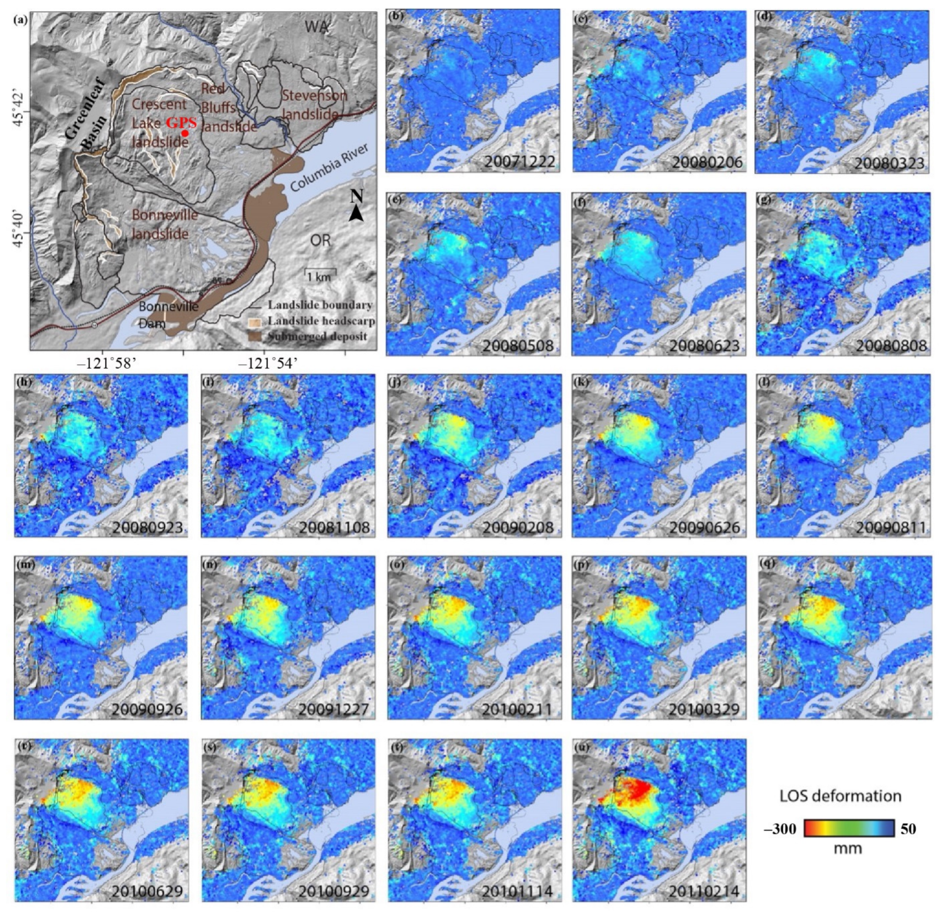
3.2.1. Cascades Landslide Complex

Columbia River Gorge in the state of Washington intrigues tourists and geoscientists by the legend of “the Bridge of the Gods”, which was a blockage dammed by ancient Bonneville Landslide deposits (Figure 3). This historic site belongs to Cascade Landslide Complex between the populated North Bonneville and Stevenson communities. Landslides often occur in the Columbia River Gorge along the steep slopes during heavy rainfall seasons (October~April), and the landslides in the western part of the Gorge are more predominant on the Washington side of the river rather than Oregon side due to the composition and structure of the underlying bedrock. The Cascades landslide complex consists of four landslides, namely Carpenters, Bonneville, Red Bluffs, and Mosley Lakes. The landslide occurs within a gently dipping sequence of weak, chemically altered volcaniclastic sedimentary rocks and minor interbedded lava flows that are overlain by more competent layers of rock [42]. The underlying sediments are composed of volcaniclastic sandstones and conglomerates of intermediate composition that range from Oligocene to early Miocene in age. The volcaniclastic units are capped by an originally thick sequence of more competent rock including Miocene flood basalts, late Miocene-to-Pliocene fluvial deposits, and localized Quaternary mafic lavas [42]. Using L-band ALOS-1 PALSAR-1 and ALOS-2 PALSAR-2, and C-band Sentinel-1A/B images, Hu et al. [42,46] mapped the movement of the landslide from 2007 to 2016 using time-series InSAR processing, conducted a thickness inversion based on the observed deformation patterns, studied the driving mechanisms of the landslide, and detected a localized avalanche.

The primary factor that controls movement and eventual runout of landslides in northwestern US is the precipitation. In case that in situ measurements of precipitation or soil moisture are not available, satellite measurements on precipitation from GPM and on soil moisture from SMAP can be used in the correlation analysis. Figure 4 shows the precipitation and soil moisture measurements from space and ground at the Cascades Landslide Complex. The satellite measurements of precipitation and soil moisture generally agree with in situ measurements (Precipitation: https://raws.dri.edu accessed on 21 April 2021 and SNOTEL soil moisture: https://www.nrcs.usda.gov/wps/portal/wcc/home/quicklinks/imap accessed on 21 April 2021; Figure 4), implying the possibility that GPM and SMAP products can be used to study landslides over a few landslide locations where in situ precipitation and soil moisture measurements are not available.

Time-series movements on the most deforming area of the Cascades Landslide Complex is illustrated in Figure 5. InSAR results during 2007–2011 and 2014 and 2016 indicate that landslide movement began shortly after the wet season started around Oct-Nov. Based on the time-series from ALOS-1 PALSAR-1 during 2007–2011 it can be inferred that sliding motion of the landslide initiated when the 30-day accumulated precipitation exceeded about 300 mm when sufficient rainfall infiltrated to the basal plane and reduced the effective stress (Figure 5) [42]. The pace and amplitude of the non-linear seasonal deformation can be quantitatively correlated with the intensity of precipitation, suggesting a hydrologically driven landslide mechanism (Figure 6).

InSAR processing of Sentinel-1A/B images during 2014–2016 presented similar deformation patterns as those during 2007–2011. InSAR time-series at a location where a continuous GPS was installed in 2014 is shown in Figure 5c. Comparison between Sentinel-1A/B and GPS shows consistency between InSAR and GPS measurements [46]. Detailed analysis of the landslide motions suggests that the landslide first experienced subsidence (primarily vertical motion) when the 30-day precipitation reached about 140 mm, followed by more drastic downslope movement when the 30-day precipitation reached about 300 mm [46] (Figure 5c).

To invert for the landslide thickness based on the mass conservation requires a 3D displacement map of the landslide. With an assumption of the motions occurred along the downhill direction on the horizontal plane (i.e., the motion component v is assumed zero in Figure 1), one can constrain pseudo-3D displacements from two independent imaging geometries (such as descending and ascending). Based on ALOS-1, ALOS-2 and Sentinel-1 observations over the Crescent Lake Landslide (upper part of the Red Bluff Landslide), the landslide thickness was estimated based on Equation (1) and its volume ranges from 660 to 820 million m³ for rheology factor f ranging between 0.5 and 1 (Figure 6) [46]. The volume estimates generally agree with the field investigations [84].

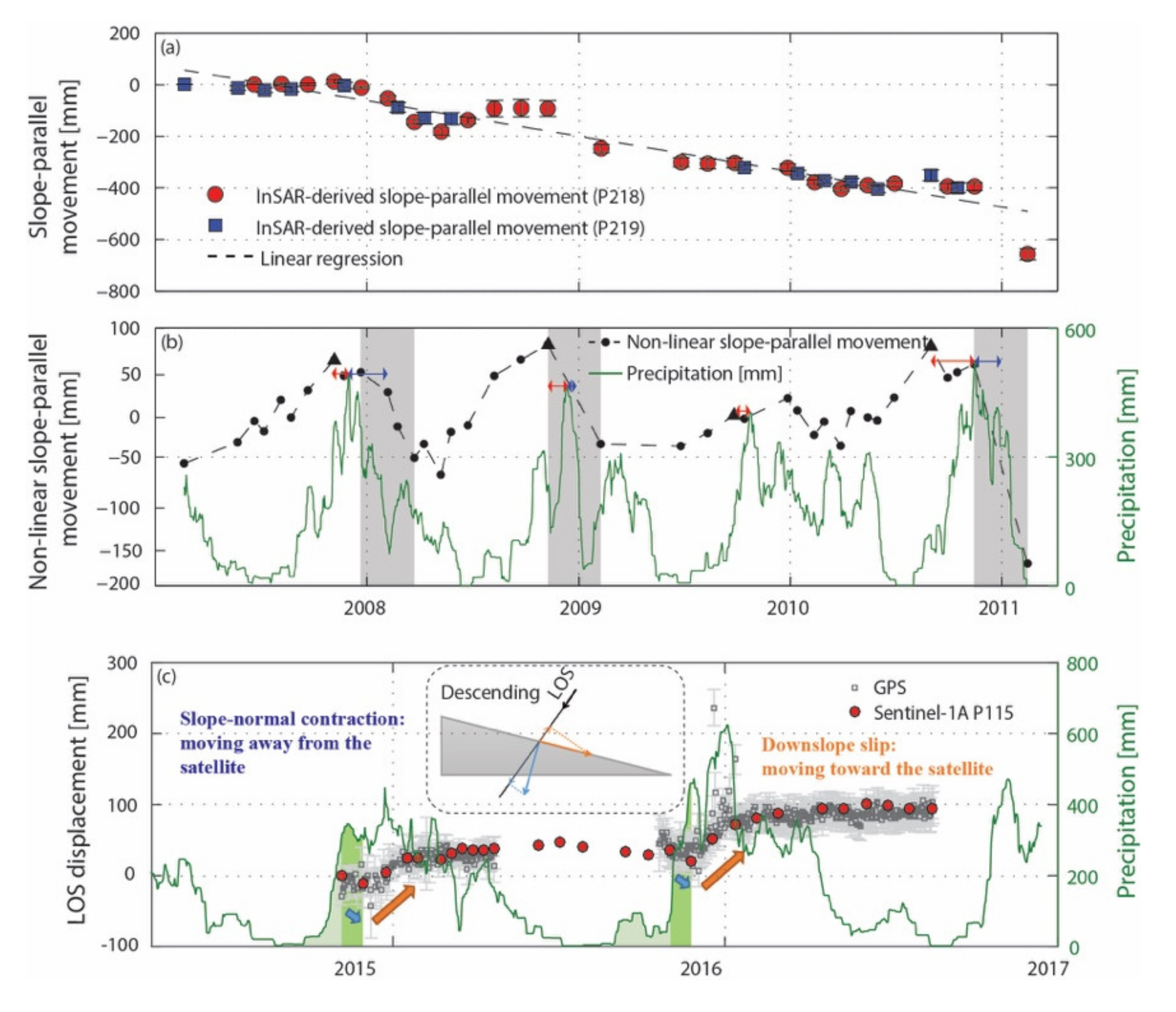
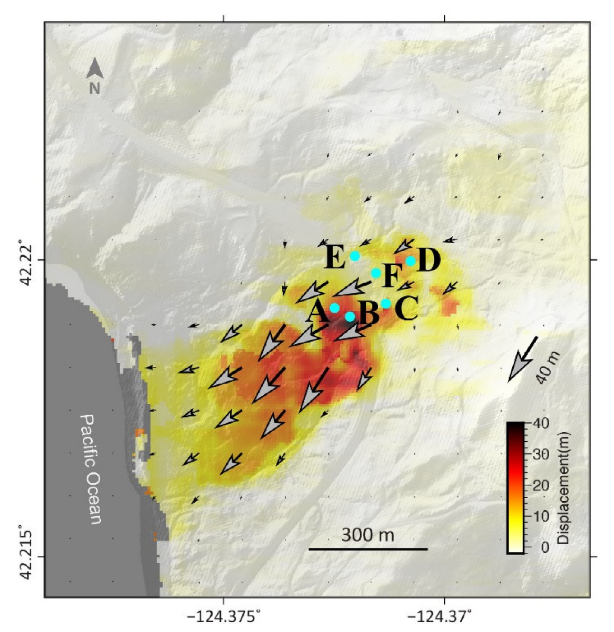
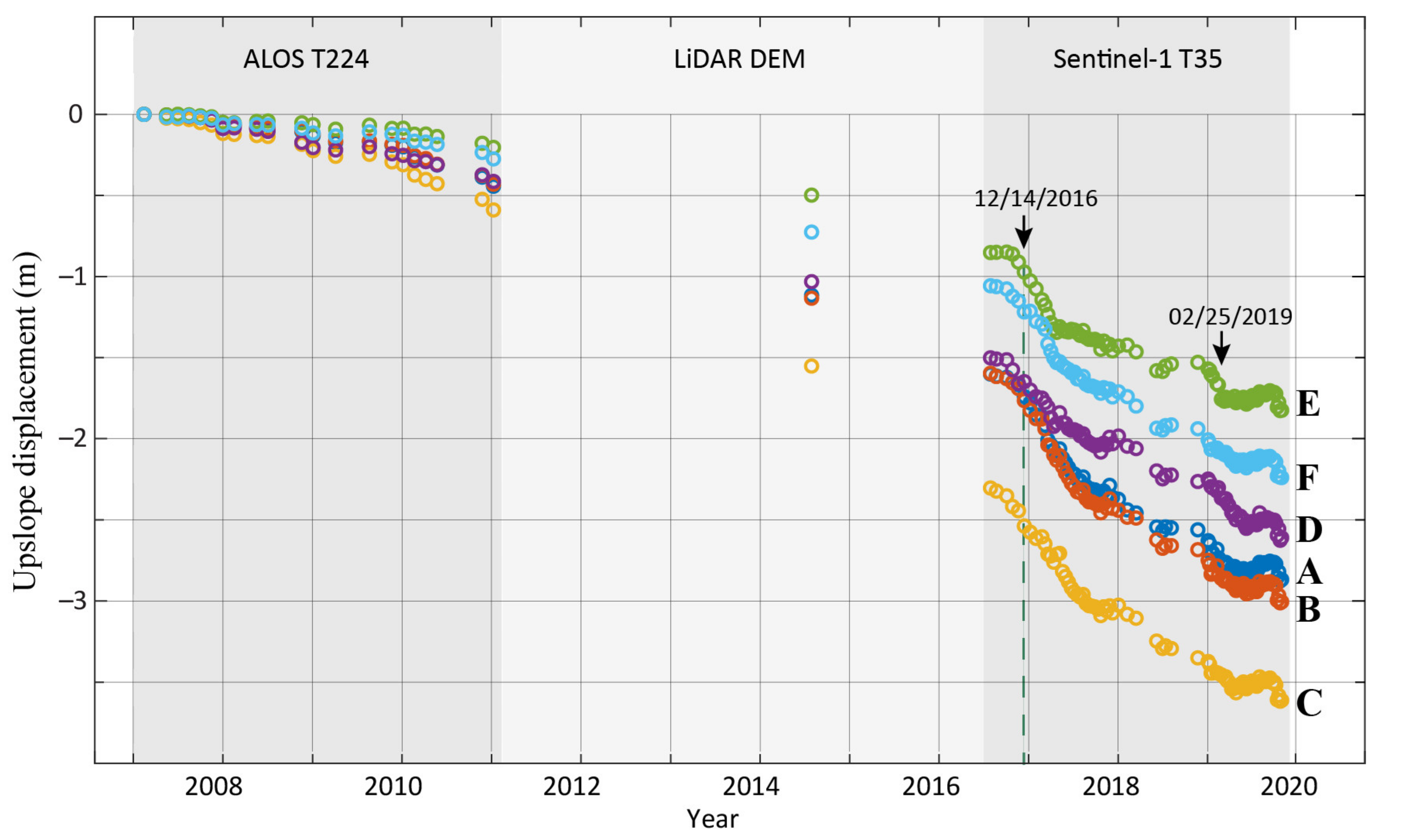
3.2.2. Hooskanaden Landslide

The Hooskanaden landslide in southwestern Oregon with large size (~600 m wide × 1300 m long) and depth (~30–45 m) has been active since at least 1958 [83]. The landslide had been in a slow motion, but occasionally caused moderated to severe damages to Highway 101. Slow movement of the landslide resulted in road repairs costing tens of thousands of dollars yearly, but a major event to destroy the highway can lead to cost beyond million dollars. The latest major collapse event occurred on 25 February 2019, which shifted the road surface about 40 m to the west and 17 m downward [83]. Consequently, the highway was closed for 13 days during the temporary repair. Materials of the slide are derived from the Otter Point Formation of Late Jurassic geologic age, which consists of sheared sandstone, mudstone, conglomerate, and interbedded sandstone and shale, with scattered BIMs (blocks-in-matrix, composed of more resistant sandstone, greenstones, chert, and blueschist). These materials, geologically referred to as mélange, accumulated as an accretionary wedge along the Cascadia subduction zone during tectonic displacement and formed the accreted western margin of the Klamath Mountains region. Stratigraphically, the slide consists of harder upper layers of predominantly sandstone and softer lower layers of mixed shale and siltstone. Hooskanaden landslide is a good example to showcase the violent nature of deep-seated landslide and thereby severe damages and collapses triggered by intense rainfall during wet season. Xu et al. [83] explored decade-long deformation of the Hooskanaden landslide based on multiple SAR (ALOS, Sentinel-1) and optical (Sentinel-2) satellites, and used multiple LiDAR DEMs to estimate the deformation rate between the ALOS and Sentinel-1 data gap. A comparison with daily rainfall and SMAP soil moisture data enhanced in-depth understanding of motion dynamics of the landslide.

Three-dimensional displacement field of the major event in 2019 was reconstructed using the pixel offset tracking of both Sentinel-1 A/B SAR data and Sentinel-2 optical satellite images [83]. When θ is the radar incidence angle and ϕ is the satellite track angle, the 3D (eastward, northward, and upward) pixelwise displacement [E N U]^T can be obtained by inverting the following equation:

$$\left[\begin{array}{ccc}\sin \varphi & \cos \varphi & 0\\ -\sin \theta \cos \varphi & \sin \theta \sin \varphi & \cos \theta \\ 0& 1& 0\\ 1& 0& 0\end{array}\right]·\left[\begin{array}{c}E\\ N\\ U\end{array}\right]=\left[\begin{array}{c}S{1}_{AZ}\\ S{1}_R\\ S{2}_N\\ S{2}_E\end{array}\right]$$

(4)

where S1_AZ, S1_R, S2_N, and S2_E are offset measurements from Sentinel-1 in azimuth and range directions and Sentinel-2 in north and east directions, respectively. The displacement map (Figure 7) retrieved from remote sensing datasets displays that the 2019 landslide event mainly moved along the downslope direction with an aspect of ~235° (clockwise from north). The middle section moved larger than head and toe sections, and its maximum horizontal displacement of ~40 m and a vertical movement of ~10 m observed from offset tracking are in a good agreement with LiDAR DEMs acquired before and after the landslide.

Historical landslide motions were revealed from the integrated use of ALOS, Sentinel-1A/B, and LiDAR DEMs [83]. Those remote sensing datasets were obtained during variant periods; ALOS PALSAR data are acquired between 2007 and 2011, Sentinel-1A/B 2016 and 2019, and LiDAR DEMs occasionally from 2008 to 2016 with varying coverage. Because there is a gap between 2011 (last acquisition of ALOS PALSAR) and 2016 (first acquisition of Sentinel-1 A/B), LiDAR DEMs were used for bridging the gap. Retrieved time-lapse (Figure 8) exhibits seasonal variations during the long-term slow movements. The slope tends to move faster during winter wet seasons and slower in the dry summer seasons. The comparison with root-zone SMAP soil moisture (averaged up to top 1 m depth) affirms the timing of accelerated landslide motion, given the increased downward water infiltration, elevated basal pore pressure, and triggered slide motion by reducing effective normal stress and consequent frictional shear resistance.

The decadal-scale landslide motion presents overall trend of apparent acceleration, with an average downslope displacement rate of ~10 cm/year from 2007–2011, ~20 cm/year from 2011 to 2016, and ~50 cm/year from 2016 to 2019 (Figure 8). The long-term acceleration is possibly caused by coastal erosion of landslide toe. Differencing LiDAR DEMs clearly demonstrate significant loss of landslide toe for years [83]. The buttressing effect of the toe to prevent abrupt collapse of the landslide body was weakened by coastal erosion, and the loss of resistance against motion of landslide body can lead to the major landslide event in 2019. Moreover, daily precipitation records of the abnormally heavy rainfall in December 2016 and February 2019 suggest that short-term but high-intensity rainfall spikes triggered major events in 2019 [83].

3.2.3. Gold Basin Landslide

The possible runout event in the Gold Basin landslide in Washington poses a direct threat to a popular campground (Gold Basin campground) located on the opposite side of the Stillaguamish River [57]. Due to the safety concerns, the campground has been closed out since 2014. In addition to a potent runout event, fine-grained sediments from the landslide complex have been transported into the South Fork Stillaguamish River and the transported materials could reduce water quality and threaten riverine ecosystem. The landslide complex consists of three small, steep tributary valleys that form three separate lobes on the north valley wall and top section (headscarp) of the landslide complex is steeply inclined with exposed soil and rocks. There have been three large historical runout events over the Gold Basin landslide complex in 1942, 1964, and 1996 [57]. Before opening the campground, the safety of the landslides complex should be assessed by the use of remote sensing datasets or other measurements. However, it is challenging to monitor the landslides using SAR datasets, because of the steep slope angles exceeding 45° that result in geometric distortion of SAR images (e.g., layover, shadow). Moreover, the size of the landslide complex is relatively small and the limited resolution of SAR images is not effective to capture movements of such small landslides. Xu et al. [57] used high-resolution SAR image to detect subtle changes over the landslide complex and simulated runout scenarios for predicting possible debris flows from the landslide complex.

Due to the steep slope in the top section of Gold Basin landslide and dense forests in middle/bottom section, phase measurements of InSAR lose coherence and do not provide any useful information. Instead, variations in SAR intensity are used to infer the surface changes due to the sliding motion, but the measurement of SAR intensity change includes uncertainties bounded by speckle noises in radar backscattering. Considering the size and slope of the landslide complex, high-resolution spotlight-mode TerraSAR-X datasets were used. Contrary to stripmap SAR acquisitions, spotlight-mode enables to obtain high-resolution (~1 m) images at cost of low spatial coverage. Further, high incidence angle of ~53° was used to overcome geometric distortion (e.g., layover). Simple differencing of multiple SAR image revealed the localized movement over the bare earth near the headscarp. The result (Figure 9) confirms that, although the displacement is not large in the spatial domain, the landslide complex is still active and needs to be cautiously monitored [57].

Based on a range of possible landslide volumes and mobility of landslide materials, scenario-based runout simulation was demonstrated (Figure 10). The simulation results suggest that debris flow with volumes less than 10⁵ m³ pose limited threats to the campground, while volumes greater than 10⁶ m³ can possibly result in severe damages [57]. When the landslide volume is low, the debris flow does not fully cross Stillaguamish River and inundates only the low plain. However, when the volume is large and the failed material is highly mobile, the debris flow affects the Gold Basin campground, which is situated on the opposite side of the valley from the landslide.

4. Discussion

4.1. Limitations of InSAR on Landslide Monitoring

InSAR is an effective method to detect landslide motions from multiple SAR acquisitions. SAR datasets include archived images (e.g., ALOS PALSAR, ERS, ENVISAT, Radarsat-1), currently operating SARs (e.g., Sentinel-1A/B, ALOS-2 PALSAR-2, TerraSAR-X, COSMO-SkyMed, Radarsat-2, SACOM) as well as airborne SAR (e.g., UAVSAR) datasets. However, when InSAR is used for the landslide mapping and monitoring, there are three major hurdles to overcome: (i) low coherence in dense vegetation, (ii) topographic errors due to human activities and natural hazards, and (iii) geometric distortion.

(i) Low coherence. The period of the most active landslides during wet season overlaps with that of low InSAR coherence. While landslides become active, the scattering characteristics are altered and the InSAR coherence consequently degrades. Therefore, there is a seasonal pattern of InSAR coherence from the northwestern US that increases in winter and decreases in summer, and the coherence tends to decrease when the terrain slope increases. Moreover, in case of highly mobile landslides or runout events, a large gradient of slope movement deteriorates InSAR coherence and cannot be consequently quantified. To avoid problems stemmed from such low InSAR coherence, the use of long-wavelength SAR datasets is preferred [34]. Except for the regions with plentiful exposed rocks and bare-earth, a short-wavelength radar signal (e.g., C- and X-band) can easily lose the InSAR coherence during wet seasons. L- (and potentially P-band) SAR datasets over the northwestern US generally keep good coherence throughout years, but C- and X-band InSAR datasets with the shortest intervals (e.g., one to two weeks) may be inadequate. Further, to cope with highly mobile landslides and better characterize each landslide in time, frequent SAR acquisitions are necessary.

(ii) Topographic errors. Most contemporary InSAR processing relies on the SRTM DEMs for topographic corrections, because it has been the most reliable near-global scale DEMs. However, the topography has been changed significantly, since the acquisition from SRTM in February 2000. The use of the old-dated DEMs can induce the error terms in the interferometric outcomes. Furthermore, the northwestern US has undergone the landslides for decades, wildfires and human activities including logging operations in Washington and Oregon have modified the mountainous landscapes that may be mis-identified as landslides. The first approach to avoid the topographic errors and thereby misidentification of landslides is to choose InSAR datasets with small perpendicular baselines. Although L- and C-band datasets can keep variable InSAR coherence up to ~2 km and ~500 m, respectively, the InSAR pairs with <100 m perpendicular baselines are preferred for landslide mapping. The use of the InSAR pairs with short baselines can limit the effects of topographic errors on the generated interferograms.

The time-series InSAR processing (e.g., PSInSAR, SBAS) also should be applied to estimate the topographic errors, but the northwestern US does not have dense observations from long-wavelength SAR datasets (e.g., ALOS-2 PALSAR-2) and utilizing the multiple InSAR pairs are not often feasible. The orbit positioning of the recent SAR datasets is well controlled inside an orbital Earth fixed tube (e.g., 50 m root-mean-square wide in radius for Sentinel-1 [85]), and using sufficient InSAR pairs with short perpendicular baselines is available. The second approach is to use the “up-to-date” topographic information in InSAR processing. The state agencies (i.e., Washington DNR, Oregon Department of Geology and Mineral Industries (DOGAMI)) have collected and distributed LiDAR DEMs with one-meter or higher resolution to the public [86]. Although the LiDAR DEMs over some landslide-prone areas are still yet to be acquired in the near future, the high-resolution DEMs can improve the quality of the InSAR landslide mapping. Additionally, one issue of statewide airborne LiDAR DEM acquisitions is that the elevation of wide area cannot be acquired at the same time but has been obtained gradually from year to year. Moreover, the already acquired LiDAR DEMs cannot be updated in a short period of time due to the difficulty of data acquisition and associated costs. If the LiDAR DEM was acquired several years ago, the topography of landslide areas is already changed significantly and the old LiDAR DEMs that do not reflect continuously changing topography can result in topographic errors in InSAR processing. Finally, it should be noted that no matter how accurate of the DEM, the average scatterer height of a SAR pixel might still deviate from the elevation defined in the DEM. In any case, for large-baseline InSAR applications in hilly and vegetated landslide settings, DEM error check with the assistance of orbital information needs to be included in the time-series analysis routine.

(iii) Geometric distortion. Due to the oblique side-looking geometry of SAR observations, the SAR images over the mountainous terrains are affected by the layover and shadow effects. When SAR images already include such effects, it is almost impossible to correct them. Choosing InSAR images from multiple tracks (e.g., ascending, descending) with less geometric distortion will be helpful for the landslide mapping. Moreover, if possible, programmed SAR acquisitions of a large incidence angle (i.e., a large incidence angle (>50°) for TerraSAR-X) can suppress the layover effects in steep terrain (>40° slope) of the northwestern US. Many landslide slopes in the northwestern US are south- or north-facing and their movement direction can be parallel to satellite moving direction. In such cases, the InSAR observation, which is insensitive to movements in the azimuth direction, cannot resolve the surface deformation in north-south direction. Offset tracking method that depends on the cross-correlation of SAR intensity can be applied to supplement the horizontal deformation [87].

In addition to three major problems, InSAR is not effective for estimating a long-term time-series deformation of fast-moving due to the characteristics of interferometric phases constrained within 2π modulo [58]. However, for identifying and mapping landslides without measuring landslide velocity, the ambiguity of InSAR measurements over fast-moving landslides is not a major issue.

Even through time-series InSAR processing such as SBAS, PSInSAR, and combination of SBAS and PSInSAR is routinely utilized in InSAR applications, we should be aware that PS targets are sparsely present in non-urban areas and even less in landslide regions with dense vegetation, rainfall, and surface runoff. However, some clusters of pixels known as distributed scatterers (DS) show moderate coherence in short-temporal-separation and small-spatial-baseline InSAR pairs. These neighboring pixels share similar reflectivity as they belong to a common geophysical target [88]. Spatially adaptive filtering approaches can be used to identify such groups of spatially homogeneous pixels (SHP). Principal component analysis of the covariance matrix for the SHPs allows for the separation of the primary scattering mechanism from those causing decorrelation given a stable InSAR phase history for the DS targets [88,89]. These DS pixels can be processed alongside PS pixels to obtain an increased number of measurement points in vegetated regions (e.g., [88]). So, DS InSAR analysis over landslide terrains is becoming an attractive research topic.

4.2. Future Developments of InSAR Studies of Landslides: Landslide Slope Stability Analysis from Physics-Based Modeling

Slope stability is defined by the balance (ratio) of resisting stress (shear strength) and driving (shear) stress on the basal plane [90]. Critical time-dependent factors, such as hydraulic conditions (soil moisture, groundwater) after precipitation, often reduce the stability of landslide by decreasing frictional resistance and the strength of materials, eventually triggering sliding events. Based on InSAR-derived time-series deformation and the basal plane geometry from InSAR inversion or field investigation, the relationship between precipitation and the onset of landslide motion can be established to empirically determine the triggering thresholds [42,46]. The ensuing fluctuations of soil moisture and groundwater after the infiltration of rainfall and increased pore water pressure, along with other geologic parameters, can be integrated through numerical simulations to assess the slope stability using approaches in Abramson et al. [91]. The slope stability analyses and simulations can help better understand the role of hydrologic forces and further assess the landslide susceptibility of the active slow-moving, deep-seated landslides on a regional scale. In the case of the 2014 Oso landslide, soil saturation and high pore-fluid pressures most likely contributed to slope failure as well as the inundation afterwards [12]. We believe dense time-series landslide movement from InSAR and GPS, precipitation and soil moisture from space and ground will allow us to explore physics-based models to understand landslide stability and failure.

5. Conclusions

Mapping landslides based on SAR imagery can be accomplished through conventional InSAR processing, time-series InSAR (SBAS, PS) processing, offset tracking, SAR intensity (and possibly coherence) changes. Each technique has its own advantages and shortcomings. Over the northwestern US, the most limiting factor in monitoring landslides with InSAR is the temporal decorrelation. Thus, robust mapping of landslides through InSAR (or time-series InSAR) is better accomplished with longer wavelength SAR in shorter repeat orbits such as ALOS-2 or future NISAR (https://nisar.jpl.nasa.gov accessed on 21 April 2021). The second influential factor in mapping landslides with InSAR is the geometric distortions (layovers and shadows); resolving layover problems requires intelligent InSAR imaging geometries. This remains a challenging topic for future research. Next, DEM-induced phase artifacts can be minimized through time-series InSAR processing or the utilization of updated DEMs (e.g., [42,46]). As landslide movements are generally localized, atmospheric artifacts with a long wavelength are not an obstacle in landslide detection although they will reduce the measurement precision.

The InSAR techniques including offset tracking and time-series intensity analysis can provide critical information about the detailed spatio-temporal slope deformations, which help infer the basal slip surface and landslide volume over the northwestern US. The conventional InSAR with acquisitions during a dry season for keeping high coherence can be used to map the active landslides with low displacement rates. As shown from the map of active deep-seated landslides in Washington, the long-wavelength ALOS-2 PALSAR-2 InSAR results can successfully identify the landslides that are difficult to be often updated by other sensors. Although the velocity of fast-moving landslides may not be accurately calculated due to the ambiguity of phase measurements [34,58], the existence of landslides still can be revealed by the use of conventional InSAR method. The activity and extent of the deep-seated landslides by InSAR can provide supplementary information to the current federal and state landslide inventory. The landslide thickness is an important parameter to calculate the landslide volume, understand dynamics of the deep-seated landslides, and forecast a possible runout event during high and/or long precipitation. Time-series InSAR measurements can be used to estimate the landslide thickness [42,46] and timing of landslide initiation and acceleration [67]. Although most deep-seated landslides may not lead to runout or avalanches, the Hooskanaden landslide that occurred in 2019 showed that a decade-long slow movement of the deep-seated landslide can result in a catastrophic slope failure and avalanches when combined with intense precipitation and coastal erosion [83]. When we can estimate the landslide volume from our measurements, the scenario-based numerical runout model can be performed for mitigating future risks of extensive landslides [57]. Precipitation and soil moisture, measured from space and ground, are key triggers in hydrology-driven landslides because of the reduced basal friction, and they help predict the onset of runout versus slow-moving landslides, and amplified landslide mobility. All measurements from space and ground should be integrated into slope stability analyses and numerical simulations under different scenarios to find the best fitting model, and to identify thresholds possibly instigating failures, given various geologic and topographic settings.

References

1. Cruden, D.M. A simple definition of a landslide. Bull. Eng. Geol. Environ. 1991, 43, 27–29. [Google Scholar] [CrossRef]
2. Korup, O.; Densmore, A.L.; Schluengger, F. The role of landslides in mountain range evolution. Geomorphology 2010, 12, 77–90. [Google Scholar] [CrossRef]
3. Larsen, I.J.; Montgomery, D.R.; Korup, O. Landslide erosion controlled by hillslope material. Nat. Geosci. 2010, 3, 247–251. [Google Scholar] [CrossRef]
4. US. Geological Survey. Landslide Hazards—A National Threat. U.S. Geological Survey Fact Sheet 2005–3156; U.S. Geological Survey: Reston, VA, USA, 2005; pp. 1–2.
5. Iversion, R.M. Landslide triggering by rain infiltration. Water Resour. Res. 2010, 36, 1897–1910. [Google Scholar] [CrossRef] [Green Version]
6. Malamud, B.D.; Turcotte, D.L.; Guzzetti, F.; Reichenbach, P. Landslide inventories and their statistical properties. Earth Surf. Proc. Land. 2004, 29, 687–711. [Google Scholar] [CrossRef]
7. Cannon, S.H.; Kirkhamb, R.M.; Parise, M. Wildfire-related debris-flow initiation processes, Storm King Mountain, Colorado. Geomorphology 2001, 39, 171–188. [Google Scholar] [CrossRef]
8. Schulz, W.H.; Kean, J.W.; Wang, G. Landslide movement in southwest Colorado triggered by atmospheric tides. Nat. Geosci. 2009, 2, 863–866. [Google Scholar] [CrossRef]
9. Highland, L.M.; Bobrowsky, P. The Landslide Handbook—A Guide to Understanding Landslides. In U.S. Geological Survey Circular 1325; U.S. Geological Survey: Reston, VA, USA, 2008; p. 129. [Google Scholar]
10. Petley, D. Global patterns of loss of life from landslides. Geology 2012, 40, 927–930. [Google Scholar] [CrossRef]
11. Iversion, R.M.; George, D.L.; Allstadt, K.; Reid, M.E.; Collins, B.D.; Vallance, J.W.; Schilling, S.P.; Godt, J.W.; Cannon, C.M.; Magirl, C.S.; et al. Landslide mobility and hazard: Implications of the 2014 Oso disaster. Earth Planet. Sci. Lett. 2015, 412, 197–208. [Google Scholar] [CrossRef] [Green Version]
12. Iversion, R.M.; George, D.L. Modelling landslide liquefaction, mobility bifurcation and the dynamics of the 2014 Oso disaster. Geotechnique 2016, 66, 175–187. [Google Scholar] [CrossRef]
13. Kim, J.W.; Lu, Z.; Qu, F.; Hu, X. Pre-2014 mudslides at Oso revealed by InSAR and multi-source DEM analysis. Geomat. Nat. Hazards Risk 2015, 6, 184–194. [Google Scholar] [CrossRef]
14. Hilley, G.E.; Bürgmann, R.; Ferretti, A.; Novali, F.; Rocca, F. Dynamics of slow-moving landslides from Permanent Scatterer Analysis. Science 2004, 304, 1952–1954. [Google Scholar] [CrossRef] [PubMed] [Green Version]
15. Mackey, B.H.; Roering, J.J. Sediment yield, spatial characteristics, and the long-term evolution of active earthflows determined from airborne LiDAR and historical aerial photographs, Eel River, California. Geol. Soc. Am. Bull. 2011, 123, 1560–1576. [Google Scholar] [CrossRef]
16. Zhao, C.; Lu, Z.; Zhang, Q.; de la Fuente, J. Large-area landslide detection and monitoring with ALOS/PALSAR imagery data over Northern California and Southern Oregon, USA. Remote Sens. Environ. 2012, 124, 348–359. [Google Scholar] [CrossRef]
17. Cevasco, A.; Termini, F.; Valentino, R.; Meisina, C.; Bonì, R.; Bordoni, M.; Cgekkam, G.P.; De Vita, P. Residual mechanisms and kinematics of the relict Lemeglio coastal landslide (Liguria, northwestern Italy). Geomorphology 2018, 320, 64–81. [Google Scholar] [CrossRef]
18. Handwerger, A.L.; Roering, J.J.; Schmidt, D.A. Controls on the seasonal deformation of slow-moving landslides. Earth Planet. Sci. Lett. 2013, 377–378, 239–247. [Google Scholar] [CrossRef]
19. Handwerger, A.L.; Rempel, A.W.; Roering, J.J.; Hilley, G.E. Rate-weakening friction characterizes both slow sliding and catastrophic failure of landslides. Proc. Natl. Acad. Sci. USA 2016, 113, 10281–10286. [Google Scholar] [CrossRef] [Green Version]
20. Terzaghi, K. Mechanism of Landslides in Application of Geology to Engineering Practice; Paige, S., Ed.; Geological Society of America: New York, NY, USA, 1950; pp. 83–123. [Google Scholar]
21. Warner, M.D.; Mass, C.F.; Salathé, E.P., Jr. Wintertime extreme precipitation events along the Pacific Northwest coast: Climatology and synoptic evolution. Mon. Weather Rev. 2012, 140, 2021–2043. [Google Scholar] [CrossRef] [Green Version]
22. NOAA National Centers for Environmental Information (NCEI). U.S. Billion-Dollar Weather and Climate Disasters; July 2019. Available online: https://www.ncdc.noaa.gov/billions/ (accessed on 21 April 2021).
23. Mastin, M.C.; Gendaszek, A.S.; Barnas, C.R. Magnitude and Extent of Flooding at Selected River Reaches in Western Washington, January 2009. In U.S. Geological Survey Scientific Investigations Report 2010–5177; U.S. Geological Survey: Reston, VA, USA, 2010; p. 34. [Google Scholar]
24. Thompson, P.W.; Cierlitza, S. Identification of a Slope Failure over a Year before Final Collapse Using Multiple Monitoring Methods. In Geotechnical Instrumentation and Monitoring in Open Pit and Underground Mining; Szwedzicki, T., Ed.; A.A. Balkema: Rotterdam, The Netherlands, 1993; pp. 491–511. [Google Scholar]
25. Ding, X.; Montgomery, S.B.; Tsakiri, M.; Swindells, C.F.; Jewell, R.J. Integrated Monitoring Systems for Open Pit Wall Deformation. In Meriwa Report No. 186; Australian Centre for Geomechanics: Crawley, Australia, 1998; pp. 3–114. [Google Scholar]
26. Zebker, H.A.; Rosen, P.A.; Goldstein, R.M.; Gabriel, A.; Werner, C.L. On the derivation of coseismic displacement fields using differential radar interferometry: The Landers earthquake. J. Geophys. Res. 1994, 99, 19617–19634. [Google Scholar] [CrossRef]
27. Massonet, D.; Briole, P.; Arnaud, A. Deflation of Mount Etna monitored by spacebrone radar interferometry. Nature 1995, 375, 567–570. [Google Scholar] [CrossRef]
28. Rosen, P.A.; Hensley, S.; Joughin, I.R.; Li, F.K.; Madsen, S.N.; Rodriguez, E.; Goldstein, R. Synthetic aperture radar interferometry. Proc. IEEE 2000, 88, 333–382. [Google Scholar] [CrossRef]
29. Bürgmann, R.; Rosen, P.A.; Fielding, E.J. Synthetic aperture radar interferometry to measure Earth’s surface topography and its deformation. Ann. Rev. Earth Planet. Sci. 2000, 28, 169–209. [Google Scholar] [CrossRef]
30. Hanssen, R. Radar Interferometry; Kluwer: Dordrecht, The Netherlands, 2001. [Google Scholar]
31. Schmidt, D.A.; Burgmann, R. Time-dependent land uplift and subsidence in the Santa Clara valley, California, from a large interferometric synthetic aperture radar data set. J. Geophys. Res. 2003, 108, 2416. [Google Scholar] [CrossRef] [Green Version]
32. Simons, M.; Rosen, P.A. Interferometric synthetic aperture radar geodesy. In Treatise on Geophysics-Geodesy; Elsevier: Amsterdam, The Netherlands, 2007; Volume 3, pp. 391–446. [Google Scholar]
33. Ferretti, A.; Monti-Guarnieri, A.; Prati, C.; Rocca, F.; Massonet, D. InSAR Principles-Guidelines for SAR Interferometry Processing and Interpretation; ESA: Noordwijk, The Netherlands, 2007; Volume 19. [Google Scholar]
34. Lu, Z.; Dzurisin, D. InSAR Imaging of Aleutian Volcanoes: Monitoring a Volcanic Arc from Space; Springer: Berlin/Heidelberg, Germany, 2014; p. 390. [Google Scholar]
35. Catani, F.; Farina, P.; Moretti, S.; Nico, G.; Strozzi, T. On the application of SAR interferometry to geomorphological studies: Estimation of landform attributes and mass movements. Geomorphology 2005, 66, 119–131. [Google Scholar] [CrossRef]
36. Strozzi, T.; Farina, P.; Corsini, A.; Ambrosi, C.; Thüring, M.; Zilger, J.; Wiesmann, A.; Wegmüller, U.; Werner, C. Survey and monitoring of landslide displacements by means of L-band satellite SAR interferometry. Landslides 2005, 2, 193–201. [Google Scholar] [CrossRef]
37. Farina, P.; Colombo, D.; Fumagalli, A.; Marks, F.; Moretti, S. Permanent scatterers for landslide investigations: Outcomes from the ESA-SLAM project. Eng. Geol. 2006, 88, 200–217. [Google Scholar] [CrossRef]
38. Bulmer, M.H.; Petley, D.N.; Murphy, W.; Mantovani, F. Detecting slope deformation using two-pass differential interferometry: Implications for landslide studies on Earth and other planetary bodies. J. Geophys. Res. Planets 2006, 111, E06S16. [Google Scholar] [CrossRef] [Green Version]
39. Pierson, T.; Lu, Z. InSAR Detection of Renewed Movement of a Large Ancient Landslide in the Columbia River Gorge, Washington. In Proceedings of the From Volcanoes to Vineyards: Living with Dynamic Landscapes, Geological Society of America 2009 Annual Meeting, Portland, OR, USA, 18–21 October 2009; p. 497. [Google Scholar]
40. Calabro, M.D.; Schmidt, D.A.; Roering, J.J. An examination of seasonal deformation at the Portuguese Bend landslide, southern California, using radar interferometry. J. Geophys. Res. Earth Surf. 2010, 115, F02020. [Google Scholar] [CrossRef]
41. Cascini, L.; Fornaro, G.; Peduto, D. Advanced low- and full-resolution DInSAR map generation for slow-moving landslide analysis at different scales. Eng. Geol. 2010, 112, 29–42. [Google Scholar] [CrossRef]
42. Hu, X.; Wang, T.; Pierson, T.C.; Lu, Z.; Kim, J.; Cecere, T.H. Detecting seasonal landslide movement within the Cascade landslide complex (Washington) using time-series SAR imagery. Remote Sens. Environ. 2016, 187, 49–61. [Google Scholar] [CrossRef] [Green Version]
43. Schlögel, R.; Doubre, C.; Malet, J.P.; Masson, F. Landslide deformation monitoring with ALOS/PALSAR imagery: A D-InSAR geomorphological interpretation method. Geomorphology 2015, 231, 314–330. [Google Scholar] [CrossRef]
44. Dong, J.; Zhang, L.; Liao, M.; Gong, J. Improved correction of seasonal tropospheric delay in InSAR observations for landslide deformation monitoring. Remote Sens. Environ. 2019, 233, 111370. [Google Scholar] [CrossRef]
45. Colesanti, C.; Ferretti, A.; Prati, C.; Rocca, F. Monitoring landslides and tectonic motions with the permanent scatterers technique. Eng. Geol. 2003, 68, 3–14. [Google Scholar] [CrossRef]
46. Hu, X.; Lu, Z.; Pierson, T.; Kramer, R.; George, D. Combining InSAR and GPS to determine transient movement and thickness of a seasonally active low-gradient translational landslide. Geophys. Res. Lett. 2018, 45, 1453–1462. [Google Scholar] [CrossRef]
47. Berardino, P.; Fornaro, G.; Lanari, R.; Sansosti, E. A new algorithm for surface deformation monitoring based on small baseline differential SAR interferograms. IEEE Trans. Geosci. Remote Sens. 2002, 40, 2375–2383. [Google Scholar] [CrossRef] [Green Version]
48. Ferretti, A.; Prati, C.; Rocca, F. Permanent scatterers in SAR interferometry. IEEE Trans. Geosci. Remote Sens. 2001, 39, 8–20. [Google Scholar] [CrossRef]
49. Hooper, A.; Zebker, H.; Segall, P.; Kampes, B. A new method for measuring deformation on volcanoes and other natural terrains using InSAR persistent scatterers. Geophys. Res. Lett. 2004, 31, L23611. [Google Scholar] [CrossRef]
50. Wang, T.; Jónsson, S. Improved SAR Amplitude Image Offset Measurements for Deriving Three-Dimensional Coseismic Displacements. IEEE J. Sel. Top. Appl. Earth Observ. Remote Sens. 2015, 8, 3271–3278. [Google Scholar] [CrossRef] [Green Version]
51. Hu, X.; Wang, T.; Liao, M. Measuring coseismic displacements with point-like targets offset tracking. IEEE Geosci. Remote Sens. Lett. 2014, 11, 283–287. [Google Scholar] [CrossRef]
52. Moro, M.; Chini, M.; Saroli, M.; Atzori, S.; Stramondo, S.; Salvi, S. Analysis of large, seismically induced gravitational deformations imaged by high resolution COSMO-SkyMed SAR. Geology 2011, 39, 527–530. [Google Scholar] [CrossRef]
53. Kim, J.W.; Lu, Z.; Gutenberg, L.; Zhu, Z. Characterizing hydrologic changes of the Great Dismal Swamp using SAR/InSAR. Remote Sens. Environ. 2017, 198, 187–202. [Google Scholar] [CrossRef]
54. Melo, R.; Asch, T.V.; Zêzere, J.L. Debris flow run-out simulation and analysis using a dynamic model. Nat. Hazards Earth Syst. Sci. 2018, 18, 555–570. [Google Scholar] [CrossRef] [Green Version]
55. Napoli, M.D.; Martire, D.D.; Bausilio, G.B.; Calcaterra, D.; Confuorto, P.; Firpo, M.; Pepe, G.; Cevasco, A. Rainfall-Induced Shallow Landslide Detachment, Transit and Runout Susceptibility Mapping by Integrating Machine Learning Techniques and GIS-Based Approaches. Water 2021, 13, 488. [Google Scholar] [CrossRef]
56. Kavoura, K.; Sabatakakis, N. Investigating landslide susceptibility procedures in Greece. Landslides 2020, 17, 127–145. [Google Scholar] [CrossRef]
57. Xu, Y.K.; George, D.L.; Kim, J.W.; Lu, Z.; Riley, M.; Griffin, T.; de la Fuente, J. Landslide monitoring and runout hazard assessment by integrating multi-source remote sensing and numerical models: An application to the Gold Basin landslide complex, northern Washington. Landslides 2020, 18, 1131–1141. [Google Scholar] [CrossRef]
58. Wasowski, J.; Bovenga, F. Remote Sensing of Landslide Motion with Emphasis on Satellite Multitemporal Interferometry Applications. In An Overview, Landslide Hazards, Risks and Disasters; Elsevier: Amsterdam, The Netherlands, 2014; pp. 345–403. [Google Scholar]
59. Hooper, A. A multi-temporal InSAR method incorporating both persistent scatterer and small baseline approaches. Geophys. Res. Lett. 2008, 35, L16302. [Google Scholar] [CrossRef] [Green Version]
60. Liu, Y.Y.; Lu, Z.; Zhao, C.Y.; Kim, J.W.; Zhang, Q.; de la Fuente, J. Characterization of the Kinematic Behavior of Three Bears Landslide in Northern California using L-band InSAR Observations. Remote Sens. 2019, 11, 2726. [Google Scholar] [CrossRef] [Green Version]
61. Casu, F.; Manconi, A.; Pepe, A.; Lanari, R. Deformation time-series generation in areas characterized by large displacement dynamics: The SAR amplitude pixel-offset SBAS technique. IEEE Trans. Geosci. Remote Sens. 2011, 49, 2752–2763. [Google Scholar] [CrossRef]
62. McKean, J.; Roering, J. Objective landslide detection and surface morphology mapping using high-resolution airborne laser altimetry. Geomorphology 2004, 57, 331–351. [Google Scholar] [CrossRef]
63. Glenn, N.F.; Streutker, D.R.; Chadwick, D.J.; Thackray, G.D.; Dorsch, S.J. Analysis of LiDAR-derived topographic information for characterizing and differentiating landslide morphology and activity. Geomorphology 2006, 73, 131–148. [Google Scholar] [CrossRef]
64. Hong, Y.; Adler, R.; Huffman, G. Evaluation of the potential of NASA multi-satellite precipitation analysis in global landslide hazard assessment. Geophys. Res. Lett. 2006, 33, L22402. [Google Scholar] [CrossRef]
65. NASA. SMAP (Soil Moisture Active Passive) Handbook: Mapping Soil Moisture and Freeze/Thaw from Space; Jet Propulsion Laboratory Publication: Pasadena, CA, USA, 2014; pp. 1–192.
66. Lu, Z.; Kim, J.; Hu, X.; Xu, Y.; George, D. Development of an Incorporated Platform to Characterize Hydrology-Driven Landslide Hazards in Northwestern US. In Proceedings of the Asia Oceania Geosciences Society 15th Annual Meeting, Honolulu, HI, USA, 3–8 June 2018. [Google Scholar]
67. Xu, Y.; Kim, J.W.; George, D.L.; Lu, Z. Seasonal rainfall-driven sliding, basal geometry, and time lag from InSAR: Lawson Creek landslide, Oregon. Remote Sens. 2019, 11, 2347. [Google Scholar] [CrossRef] [Green Version]
68. Okada, Y. Surface deformation due to shear and tensile faults in a half space. Bull. Seismol. Soc. Am. 1985, 75, 1135–1154. [Google Scholar]
69. Aryal, A.; Benjamin, A.B.; Reid, M.E. Landslide subsurface slip geometry inferred from 3-D surface displacement fields. Geophys. Res. Lett. 2015, 42, 1411–1417. [Google Scholar] [CrossRef]
70. Nikolaeva, E.; Walter, T.R.; Shirzaei, M.; Zschau, J. Landslide observation and volume estimation in central Georgia based on L-band InSAR. Nat. Hazards Earth Syst. Sci. 2014, 14, 675–688. [Google Scholar] [CrossRef] [Green Version]
71. Booth, A.M.; Lamb, M.P.; Avouac, J.P.; Delacourt, C. Landslide velocity, thickness, and rheology from remote sensing: La Clapière landslide, France. Geophys. Res. Lett. 2013, 40, 1–6. [Google Scholar] [CrossRef] [Green Version]
72. Delbridge, B.; Burgmann, R.; Fielding, E.; Hensley, S. Kinematics of the Slumgullion Landslide from UAVSAR Derived Interferograms. In Proceedings of the 2015 IEEE International Geoscience and Remote Sensing Symposium (IGARSS), Milan, Italy, 26–31 July 2015; IEEE: Piscataway, NJ, USA, 2015; pp. 3842–3845. [Google Scholar]
73. Reid, M.E. A pore-pressure diffusion model for estimating landslide-inducing rainfall. J. Geol. 1994, 102, 709–717. [Google Scholar] [CrossRef]
74. Boggard, T.A.; Greco, R. Landslide hydrology: From hydrology to pore pressure. WIREs Water 2016, 3, 439–459. [Google Scholar] [CrossRef]
75. Hu, X.; Bürgmann, R.; Lu, Z.; Handwerger, A.L.; Wang, T.; Miao, R.Z. Mobility, thickness, and hydraulic diffusivity of the slow-moving Monroe landslide in California revealed by L-band satellite radar interferometry. J. Geophys. Res. 2019, 124, 7504–7518. [Google Scholar] [CrossRef] [Green Version]
76. Kang, Y.; Lu, Z.; Zhao, C.Y.; Xu, Y.K.; Kim, J.W.; Gallegos, A.J. InSAR Monitoring of Creeping Landslides in Mountainous Regions: A Case Study in Eldorado National Forest, California. Remote Sens. Environ. 2021, 258, 112400. [Google Scholar] [CrossRef]
77. George, D.L.; Iversion, R.M. A depth-averaged debris-flow model that includes the effects of evolving dilatancy: 2. Numerical predictions and experimental tests. Proc. R. Soc. A 2014, 470, 2170. [Google Scholar] [CrossRef] [Green Version]
78. Orr, E.L.; Orr, W.N. Oregon Geology, 6th ed.; Oregon State University Press: Corvalis, OR, USA, 2012. [Google Scholar]
79. Cheney, E.S. Chapter 3: Overview of the Geology of Washington in the Geology of Washington and Beyond; University of Washington Press: Seattle, WA, USA, 2015; pp. 18–20. [Google Scholar]
80. Wieczorek, G.F. Preparing a detailed landslide-inventory map for hazard evaluation and reduction. Environ. Eng. Geosci. 1984, XXI, 337–342. [Google Scholar] [CrossRef]
81. Bonì, R.; Bordoni, M.; Colombo, A.; Lanteri, L.; Meisina, C. Landslide state of activity maps by combining multi-temporal A-DInSAR (LAMBDA). Remote Sens. Environ. 2018, 217, 172–190. [Google Scholar] [CrossRef]
82. Stanley, T.A.; Kirschbaum, D.B. Effects of inventory bias on landslide susceptibility calculation. In Proceedings of the 3rd North American Symposium on Landslides, Roanoke, VA, USA, 4–8 June 2017. [Google Scholar]
83. Xu, Y.; Lu, Z.; Schulz, W.H.; Kim, J.W. Twelve-year dynamics and rainfall thresholds for alternating creep and rapid movement of the Hooskanaden landslide from integrating InSAR, pixel offset tracking, and borehole and hydrological measurements. J. Geophys. Res. Earth Surf. 2020, 125, e2020JF005640. [Google Scholar] [CrossRef]
84. Randall, J.R. Characterization of the Red Bluff Landslide, Greater Cascade Landslide Complex, Columbia River Gorge, Washington. Master’s Thesis, Portland State University, Portland, OR, USA, 2012. [Google Scholar]
85. Peter, H.; Jäggi, A.; Fernández, J.; Escobar, D.; Ayuga, F.; Arnold, D.; Wermuth, M.; Hackel, S.; Otten, M.; Simmons, W.; et al. Sentinel-1A—First precise orbit determination results. Adv. Space Res. 2018, 60, 879–892. [Google Scholar] [CrossRef]
86. Booth, A.M.; Roering, J.J.; Perron, J.T. Automated landslide mapping using spectral analysis and high-resolution topographic data: Puget Sound lowlands, Washington, and Portland Hills, Oregon. Geomorphology 2009, 109, 132–147. [Google Scholar] [CrossRef]
87. Handwerger, A.L.; Fielding, E.J.; Huang, M.-H.; Bennett, G.L.; Liang, C.; Schulz, W.H. Widespread initiation, reactivation, and acceleration of landslides in the northern California Coast Ranges due to extreme rainfall. J. Geophys. Res. Solid Earth 2019, 24, 1782–1797. [Google Scholar] [CrossRef] [Green Version]
88. Ferretti, A.; Fumagalli, A.; Novali, F.; Prati, C.; Rocca, F.; Rucci, A. A new algorithm for processing interferometric data-stacks: SqueeSAR. IEEE Trans. Geosci. Remote Sens. 2011, 49, 3460–3470. [Google Scholar] [CrossRef]
89. Fornaro, G.; Verde, S.; Reale, D.; Pauciullo, A. CAESAR: An approach based on covariance matrix decomposition to improve multibaseline- multitemporal interferometric SAR processing. IEEE Trans. Geosci. Remote Sens. 2015, 53, 2050–2065. [Google Scholar] [CrossRef]
90. Davies, T. Hazards and Disaster Series: Landslide Hazards, Risks, and Disasters; Academic Press: Cambridge, MA, USA, 2015. [Google Scholar]
91. Abramson, L.W.; Boyce, G.M.; Thomas, S.; Sharma, S. Slope Stability and Stabilization Methods, 2nd ed.; Wiley: New York, NY, USA, 2002. [Google Scholar]
Figure 1. The configuration of landslide body. The landslide basal topography is modeled as a plane that defines the coordinates for the horizontal motion vector u and v of the slide and the vertical motion vector w. The thickness of landslide h goes through the lower yield zone and the overlying plug region: in the yield zone, the materials deform viscously with zero velocity at the basal plane; in the plug region, the materials move uniformly as a plug with no shear strain.
Geohazards 02 00002 g001
Figure 2. (a) Comparison of InSAR-observed landslides (red-outlined polygons) in Washington and landslide inventory (blue-outlined polygons) from Washington Department of Natural Resources (DNR; https://geologyportal.dnr.wa.gov accessed on 21 April 2021). (b) An enlarged region (box in Figure 2a) illustrates the differences in detail. Landslide inventory (blue polygon) displays the location and extent of past landslides of all kinds (avalanches, runout, deep-seated landslides) but InSAR observation (red polygon) presents those of currently active deep-seated landslides.
Geohazards 02 00002 g002
Figure 3. (a) Map of Cascade Landslide Complex in Washington (yellow star in Figure 2a), composed of Bonneville landslide, Red Bluff landslide (including the reactivated Crescent Lake landslide), and Stevenson landslide and others. (bu) PSInSAR-derived time-series deformation over the Cascades Landslide Complex along radar line-of-sight (LOS) from ALOS-1 PALSAR-1 during 2007 and 2011 [42]. The color scale shows LOS deformation in mm, with relatively stable areas (within ±20 mm) in blue. The warm colors (red, yellow) indicate the reactivated portions of the landslides.
Geohazards 02 00002 g003
Figure 4. (a) Comparison between daily satellite-based (i.e., GPM) and in situ (at station Three Corner Rock: https://wrcc.dri.edu/cgi-bin/rawMAIN.pl?waWTCR accessed on 21 April 2021) measurements of precipitation over the Cascades Landslide Complex. (b) Comparison between satellite-based (SMAP) and in situ (at station Log Creek) measurements of soil moisture over the Cascades Landslide Complex. GPM measurements have been provided since 13 March 2014 and SMAP soil moisture from 31 March 2015. In situ measurements of precipitation and soil moisture were made at a specific location, but both satellite measurements were calculated within a coarse resolution of 0.1° (GPM) and 9 km (SMAP).
Geohazards 02 00002 g004
Figure 5. (a) Comparison of InSAR-derived slope-parallel movement derived from ALOS-1 tracks P218 (red circles) and P219 (blue squares) at a location on the active Crescent Lake landslide (red dot in Figure 3). The black dashed line denotes the linear regression of time-series displacement. (b) InSAR-derived non-linear slope-parallel movement (black dashed line; left axis) compared with the 30-day accumulated precipitation total (green line; right axis). Black triangles depict the initiation of downslope motion, red arrows show the gaps between the initiation of downslope motion and the precipitation peaks, gray bars indicate the sliding acceleration timespan that can be determined by the existing measurements, in which higher data sampling rate contributes to narrower bars and more precise estimates, and blue arrows show the gaps between the precipitation peak and the midpoint of sliding acceleration [42]. (c) Landslide displacements from a GPS station (red dot in Figure 1), which was temporally installed and operated by USGS, projected onto the LOS direction in comparison with the Sentinel-1A measurements from descending track P115, along with pre-30-day cumulative precipitation (summation of 30 daily precipitation before each date) from a nearby weather station. The light green shades under the pre-30-day precipitation curves show the antecedent rainfall period, and the dark green shading corresponds to the period of slope-normal subsidence when the precipitation is more intense. The inset diagram shows how ground displacement is sensed by a descending right-looking satellite track [46].
Geohazards 02 00002 g005
Figure 6. (a) Displacement velocity maps of Crescent Lake landslide. (b) Landslide thickness with rheology parameter f = 2/3. (c) Profiles of surface elevation and landslide basal surface elevations with different rheology parameters along the transect P-P’ shown in (b) [46].
Geohazards 02 00002 g006
Figure 7. Three-dimensional displacement field of the February 2019 movement of the Hooskanaden landslide reconstructed from Sentinel-1/Sentinel-2 pixel offset tracking [83].
Geohazards 02 00002 g007
Figure 8. Long-term deformation of the Hooskanaden landslide from 2007 to 2019. Cumulative along-slope displacements of multiple points (cyan dots in Figure 7) of the Hooskanaden landslide [83].
Geohazards 02 00002 g008
Figure 9. TerraSAR-X intensity change between 2017 and 2018 (a) and between 2018 and 2019 (b) in the Gold Basin landslide. Cool color indicates intensity decrease and warm color intensity decrease [57].
Geohazards 02 00002 g009
Figure 10. Maximum inundation zone of the campground as m0mcrit = −0.02 meaning that landslide body is highly mobile (m0 and mcrit are initial and critical solid volume fraction of sediment). V denotes volumes ranging from 5.7 × 10⁴ to 4.5 × 10⁶ m3, and t is timestamp [57].
Geohazards 02 00002 g010
Publisher’s Note: MDPI stays neutral with regard to jurisdictional claims in published maps and institutional affiliations.