
Displacement Analyses for a Natural Slope Considering Post-Peak Strength of Soils


1
Graduate School of Architecture and Interior Design, Shu-Te University, Kaohsiung City 82445, Taiwan
2
Department of Civil Engineering, National Cheng Kung University, Tainan City 70101, Taiwan
*
Author to whom correspondence should be addressed.
GeoHazards 2021, 2(2), 41-62; https://doi.org/10.3390/geohazards2020003
Submission received: 7 March 2021
/
Revised: 15 April 2021
/
Accepted: 29 April 2021
/
Published: 1 May 2021
Abstract
:A natural slope undergoing recurrent movements caused by rainfall-induced groundwater table rises is studied using a novel method. The strength and displacement parameters are back-calculated using a force-equilibrium-based finite displacement method (FFDM) based on the first event of slope movement recorded in the monitoring period. Slope displacements in response to subsequent rainfall-induced groundwater table rises are predicted using FFDM based on the back-calculated material parameters. Important factors that may influence the accuracy of slope displacement predictions, namely, the curvature of the Mohr-Coulomb (M-C) failure envelope and post-peak strength softening, are investigated. It is found that the accuracy of slope displacement predictions can be improved by taking into account post-peak stress-displacement relationship in the analysis. The accuracy of slope displacement predictions is not influenced by the curvature of the M-C failure envelope in the displacement analysis.
1. Introduction
Intensive rainfall causes geohazards in the form of slope failures and debris flows such as those reported by Huang et al. [1,2,3,4,5]. To investigate the failure mechanism of slopes, limit equilibrium methods are widely used in which a single value of input soil strength (called operational strength or weighted strength) [6,7] is used to calculate a safety factor (Fs) for the studied slopes [8,9]. The calculated value of Fs reflects the safety margin of the slope against failure, providing no information on the deformation (or displacements) of the slopes. To remedy this shortcoming, Huang et al. [10,11] proposed a force-equilibrium-based finite displacement method (FFDM) that incorporates a nonlinear (hyperbolic) stress-displacement constitutive law for the geomaterial along the sliding surface, as shown in Figure 1. Hyperbolic curves are widely used for simulating the stress-strain and stress-displacement relationships of soils and the interface between soil and other materials [12,13,14], with the drawback that post-peak strength deterioration for some soils, as shown in Figure 2, cannot be properly accounted for. Tatsuoka et al. [14] showed the effectiveness of utilizing generalized hyperbolic equations and an exponential function for simulating the post-peak strength softening of sandy soils. However, a general description of the post-peak stress-strain (or stress-displacement) relationship is currently unavailable. A critical issue in slope stability analyses is the selection of the operation strength, i.e., the selection of a representative value of the friction angle among the peak, fully softened, and residual friction angles for the geomaterial comprising the sliding surface [15,16]. A conventional limit-equilibrium-based approach produces a back-calculated friction angle based on a known (or assumed) value of the cohesion intercept (c) under the condition of Fs = 1.0 (e.g., Huang) [17]. The result of back-analysis is not affected by the extent of slope deformation (or displacement). To correctly reflect the displacement status of the slope, Huang et al. [11,17] proposed a back-analysis approach that uses FFDM for slopes undergoing periodic slope movements induced by rainfall (or groundwater table rises). Both strength- and displacement-related parameters back-calculated from the first event of slope displacement were found to be valid for predicting slope displacements that occurred in subsequent rainfall events (or groundwater table rises). In their studies, linear Mohr-Coulomb (M-C) envelopes and hyperbolic stress-displacement relationship were used; however, this may be insufficient to properly simulate the behavior of soils. The present study aims to solve the above problem by using curved M-C envelopes and the hyperbolic stress-displacement relationship with post-peak softening.
Various hillside disasters, not only for social and economic factors, pay a heavy price, but also endanger the ecological environment. This study is proposing, as a reference in practical application and early warning work, and it is also expected that the slope disasters in the future can be significantly reduced. Results of this study preliminarily show that there is a good agreement between the calculated and the measured displacements in the studied slopes. However, obtaining more observed data on well-monitored slopes is needed so that the technique can be further verified.
2. Methodology
Observing the slope failure in natural slope and a series of rainfall tests, the mechanism of slope displacement of rainfall-induced groundwater table rises will be deserving of studying and discussing.
2.1. Constitutive Law for Stress-Displacement Relationship
The following hyperbolic equation is used for the normalized shear stress (τ/τf) vs. shear displacement (Δ) relationship along a potential failure surface (Figure 1):
where
- kinitial: initial shear stiffness
- Rf: ratio between failure strength and asymptotic shear strength
- τult: asymptotic strength at infinite displacement
- τf: failure shear strength expressed using the M-C failure criterion
The initial shear stiffness can be expressed as a power function of effective normal pressure (σ’n) on the failure surface:
where
- K: stiffness number (an experimental constant)
- PA: atmospheric pressure (=101.3 kPa)
- G: reference shear stiffness (=101.3 kPa/m)
Equations (1)–(6) are incorporated into FFDM with additional force and/or moment equilibrium equations and displacement compatibility functions for a vertically sliced failure mass to calculate the shear displacement along the failure surface (discussed below).
2.2. Internal Friction Angle of Soils
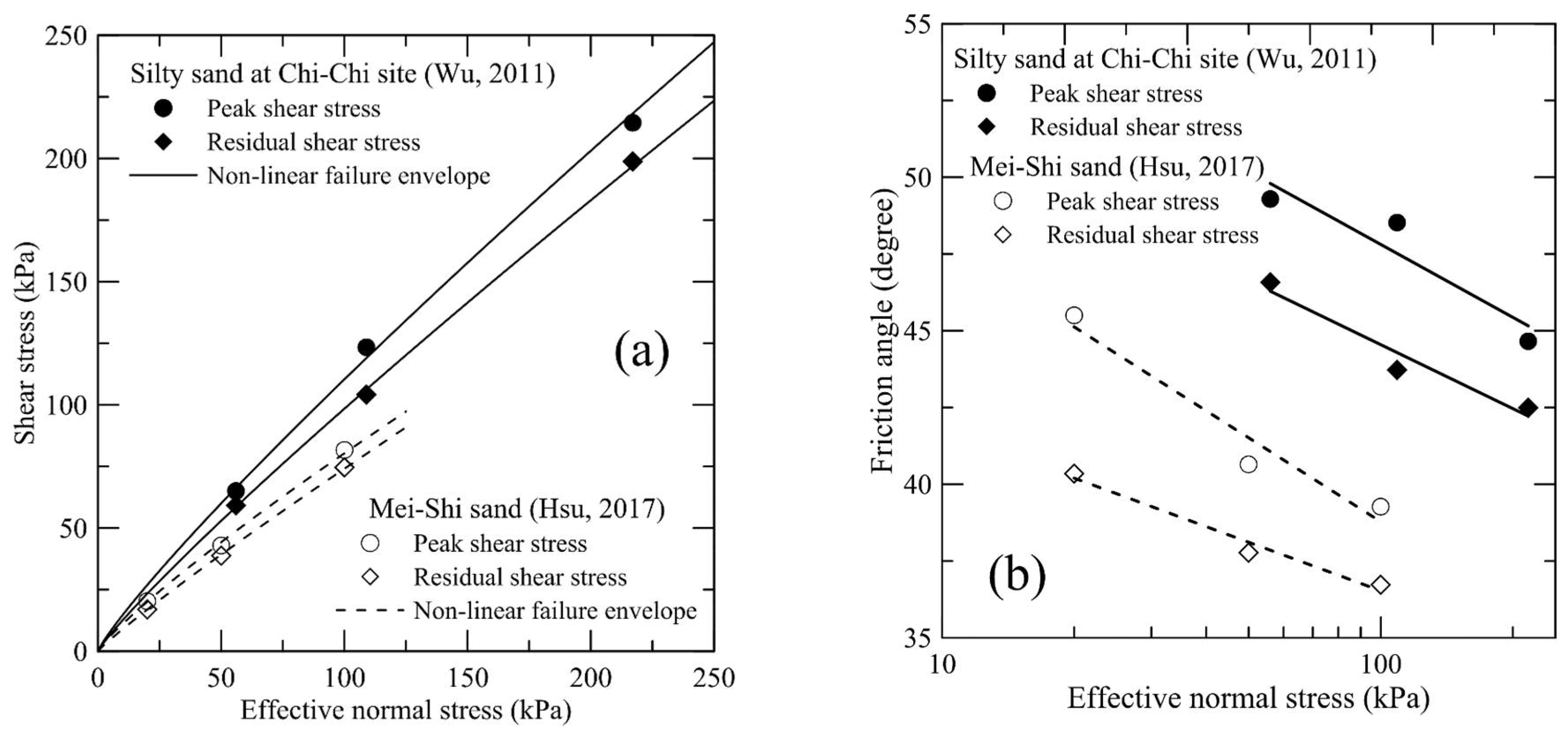
Figure 3a shows the failure envelopes for two typical sandy soils reported by Wu et al. [18,19]; these results were obtained using a medium-scale direct shear test apparatus. These failure envelopes are curved rather than straight. The following two methods are equally effective for handling the nonlinearity of the M-C failure envelope: (1) expressing the shear stress (τ) vs. normal stress (σn) relationship using a nonlinear equation [20] and (2) using a pressure-level-dependent internal friction angle, φ [21]. The latter approach is used in the present study. Figure 3b shows the φ vs. log (σn’) relationship for the data shown in Figure 3a. The straight lines can be expressed using the following equations:
where
- σn: effective normal pressures
Figure 3.
Typical results of direct shear tests: (a) Curved M-C failure envelopes and (b) Friction angles as logarithmic function of effective normal pressures.
Figure 3.
Typical results of direct shear tests: (a) Curved M-C failure envelopes and (b) Friction angles as logarithmic function of effective normal pressures.
2.3. Post-Peak Stress-Displacement Relationship
The post-peak segment of the τ vs. Δ curve is simulated in the following using a curve (also called “Versoria” or “the witch of Agnesi”) proposed by Grandi in the 1700s [22], shown in Figure 2. To use this curve efficiently as part of the stress-displacement curve, a normalized local coordinate system (X-Y coordinates) is used. The axis of X = 0 (the ordinate) passes through the point of peak stress (τf). The axis of Y = 0 (the abscissa) is an asymptote of the residual stress τr (=(1−t)·τf). A feature of this curve is that a residual state is attained at an infinite value of Δ. In practice, however, an experimental value of Δ (namely, Δr at X = 1) can be used to mimic the value of τr at a finite displacement Δr with a negligibly small error of τr. In general, the post-peak shear stress (τ) can be expressed as:
where
- t: normalized strength deterioration from peak to residual states
- Y: normalized post-peak shear stress
- X: normalized post-peak shear displacement parameter
- Δf: shear displacement at peak stress states
Values of t for various soils derived based on the reported stress-displacement curves [18,19,23,24,25,26,27,28] are summarized in Figure 4a. The values of t vary over a range of 0.1 to 0.5 for various soils. For a specific soil, values of t can be expressed as a linear function of confining stress, σn. Among the test results shown in Figure 4a, those for two direct shear tests conducted in regions of central Taiwan, reported by Wu [18] and Hsu [19] (see Figure 3a,b) are plotted in Figure 4b. The linear functions shown in Figure 3b and Figure 4b are used in the following discussions.
Based on the results of medium- or large-scale direct shear tests on various granular materials [19,23,24,25,26,27,28], the shear displacement at residual states (Δr) can be expressed as a function of the shear displacement at the peak strength state (Δf) as:
where Δratio is the ratio between the shear displacement at the residual state and that at the peak state. Values of Δratio obtained in various studies are shown in Figure 5. As can be seen, Δratio can be assumed as a linear function of σn. For a specific soil, Δratio can be expressed as:
where
- Δratio(100): value of Δratio under reference confining pressure of σn = 100 kPa
- R: experimental parameter (ranging from 0 to 0.013)
Figure 5.
Experimental values of Δratio obtained in various studies.

Figure 6 and Figure 7 compare experimental and simulated shear stress vs. displacement curves for the tests reported by Wu [18] and Hsu [19], respectively. The input parameters used for simulating the stress-displacement curves in these figures are summarized in Table 1 and Table 2, respectively. It can be seen that the simulated pre-peak and post-peak curves agree well with the experimental ones.
2.4. Displacement Compatibility Requirements
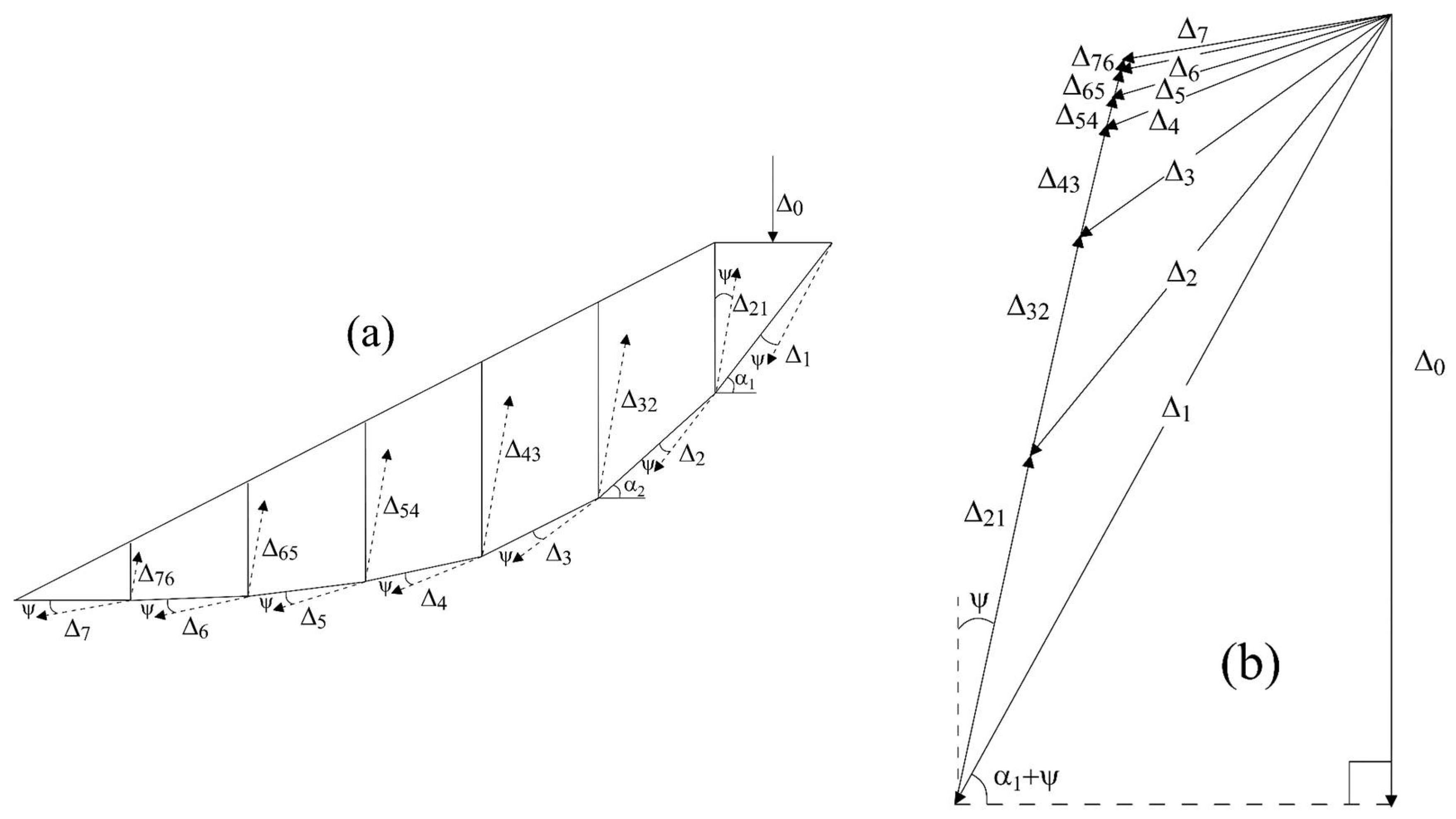
Figure 8a schematically shows an example of a potential failure surface with seven vertical slices, for which vectors of shear displacements at the slice base and the slice interface are shown in Figure 8b. Based on the hodograph shown in Figure 8c, a general expression for the shear displacement Δi (i = 1–7) at the base of slice i can be expressed as:
where
- Δ0: vertical displacement at the crest of slice 1;
- α1, αi: inclination angles for slices 1 and i, respectively
- Ψ: angle of dilation.
Figure 8.
(a) Example of sliced potential failure mass; (b) Vector of displacements along failure surface and inter-slice faces for ψ > 0 and (c) Hodogram for ψ > 0.
Figure 8.
(a) Example of sliced potential failure mass; (b) Vector of displacements along failure surface and inter-slice faces for ψ > 0 and (c) Hodogram for ψ > 0.
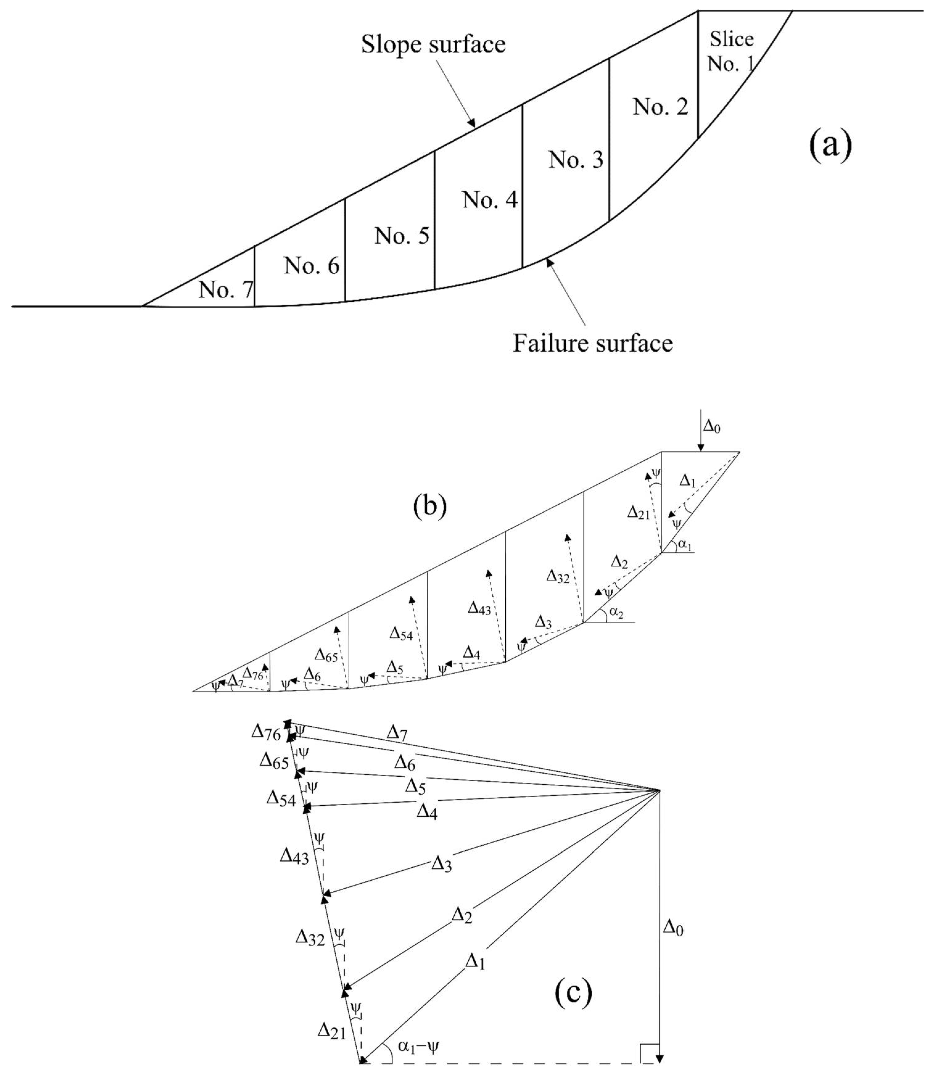
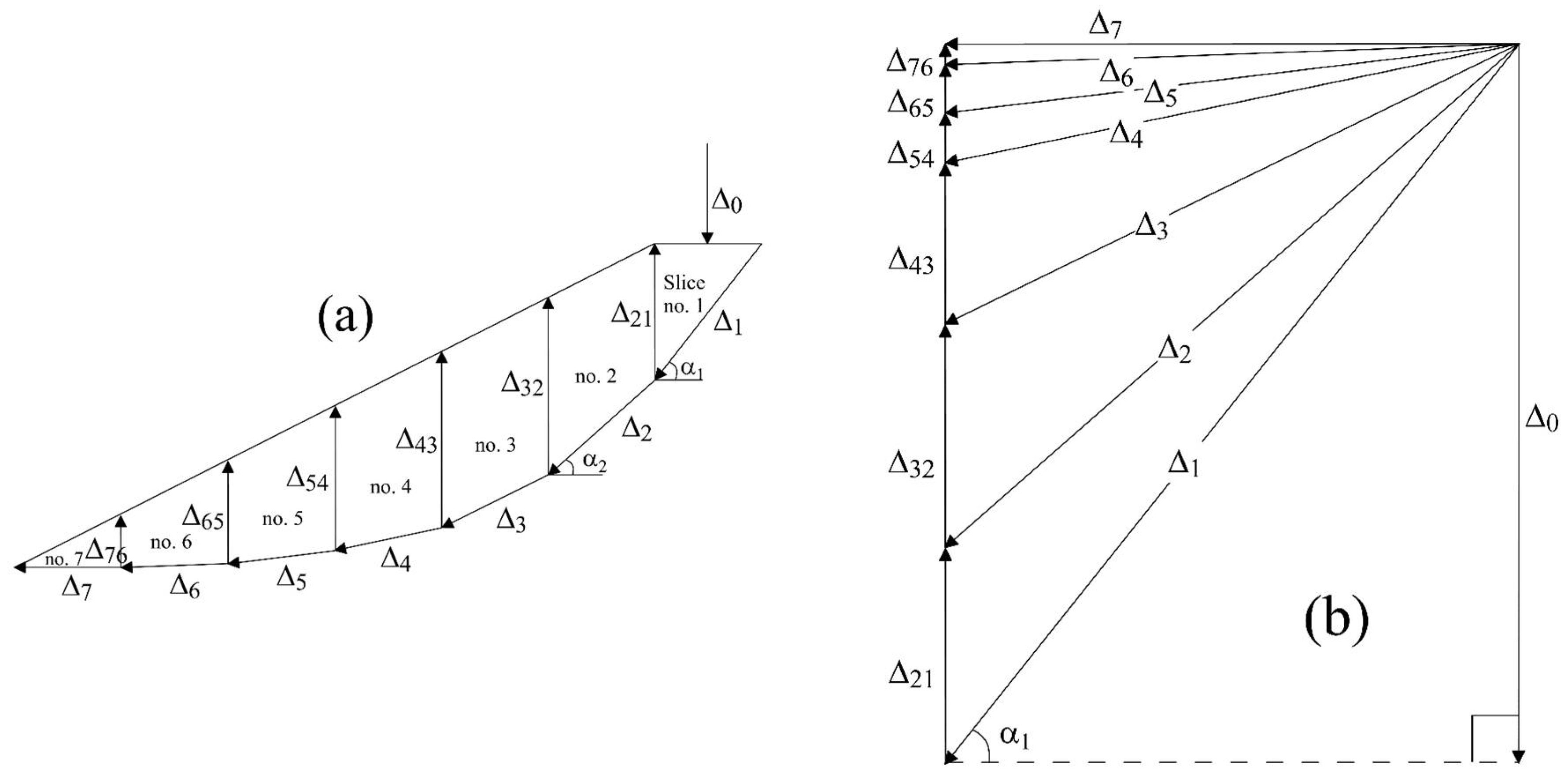
Figure 8b,c are for the case of Ψ > 0°, representing a volume expansion condition at the pre-peak state for dense soils. It can be seen that Δi increases from the crest of the slope towards the toe. Figure 9a,b show the displacement vectors and hodograph, respectively, for the case of Ψ < 0°, representing a volume contraction condition for loose soils. It can be seen that the shear displacement decreases from the crest of the slope toward the toe. The displacement vectors and hodograph for a special case of Ψ = 0° is shown in Figure 10a,b, representing a non-volume change condition at large shear displacements along the failure surface. A feature for the condition of Ψ = 0° is equal horizontal components for Δi (i = 1–7).
2.5. Calculating Safety Factors Using Method of Slices
A conventional limit equilibrium method of slices, namely Janbu’s generalized procedure of slices [29], which satisfies force and moment equilibrium requirements, is used to calculate Fs for the studied slope. For a potential sliding surface, shown in Figure 11, the differential horizontal inter-slice forces (ΔEi) can be formulated based on the vertical and horizontal force equilibrium:
where
- Wi: self-weight of slice i (i = 1−n)
- αi: base inclination of slice i
- ΔXi: differential vertical inter-slice force for slice i (=Xi−Xi−1)
- Sfi: ultimate shear strength at the base of slice i based on the M-C failure criterion.
Figure 11.
Forces acting on vertical slice of potential failure mass (Janbu’s slice method).

Equation (5), expressed by the following equation:
where Ci: cohesive resistance at slice i (=ci·li; li: length of the base of slice i).
A summation of Equation (10) yields the following equation:
where Eo, En: horizontal boundary forces at slices 0 and n, respectively.
By combining Equations (16) and (19), a constant value of Fs can be derived as:
Based on the moment equilibrium about the center of the slice base and eliminating the differential terms of Ei and Xi, which become negligibly small when slice widths are sufficiently small, one can obtain:
To calculate a constant value of Fs for a potential sliding mass with an arbitrary shape of the shear surface, initial values of Fs = 1.0 and ΔXi = 0 (i = 1−n) were used to derive approximate values of Sfi (Equation (18)) and ΔEi (Equation (16)). Improved values of Fs can be calculated (Equation (20)) using values of ΔXi (based on values of Xi from Equation (21)) until Fs converges with a tolerable convergence error of 0.5%.
2.6. Force-Equilibrium-Based Finite Displacement Method
The modified slice method introduced above is incorporated into FFDM by using a local factor of safety (Fsi) in lieu of a constant value of Fs in Equations (16), (18), and (20). By using local factors of safety (Fsi) instead of a constant one (Fs), the shear stress vs. shear displacement relationship shown in Equations (1)–(6), and the displacement compatibility function shown in Equations (14) and (15), the force system for the sliced failure mass is in a static indeterminate condition [10]. Note that Equation (1) is a reversed form of Fsi:
or
where
- τfi, τi: ultimate (or peak) shear strength and shear stress, respectively, at the base of slice i (i = 1−n)
- Sfi, Si: ultimate (or peak) shear resistance and shear force, respectively, at the base of slice i
- li: length of the base of slice i.
The Equation for Sfi (Equation (18)) can be rewritten based on the M-C failure criterion as follows:
Rewriting Equation (16) to take into account the local factor of safety (Fsi) yields:
By substituting Equations (14) and (23) into Equation (25) and summing up ΔEi (i = 1−n; Equation (17)), a closed form solution for Δ0 can be obtained:
Equation (26) can be rewritten by incorporating the M-C failure criterion, i.e., substituting Equation (24) into Equation (26):
Note that Equation (27) is a nonlinear equation, requiring a few iterative computations to derive a converged value of Δ0. To calculate Δ0, a small value of Δ0 (=0.001 m) is first used on the right-hand side of Equation (27); improved values of Fsi, ΔEi, and ΔXi are subsequently calculated using Equations (22), (25), and (21), respectively. This process is iterated until Δ0 converges. In the following analyses, an allowable convergence error of 2% is used for deriving a final value of Δ0.
The incremental slope displacement at the base of slice No. i ( ) induced by a rainfall-induced groundwater table rise (or a porewater pressure increase) can be expressed as the difference between the post-rainfall slope displacement () and the pre-rainfall slope displacement ():
3. Case Study: Lu-Shan Slope
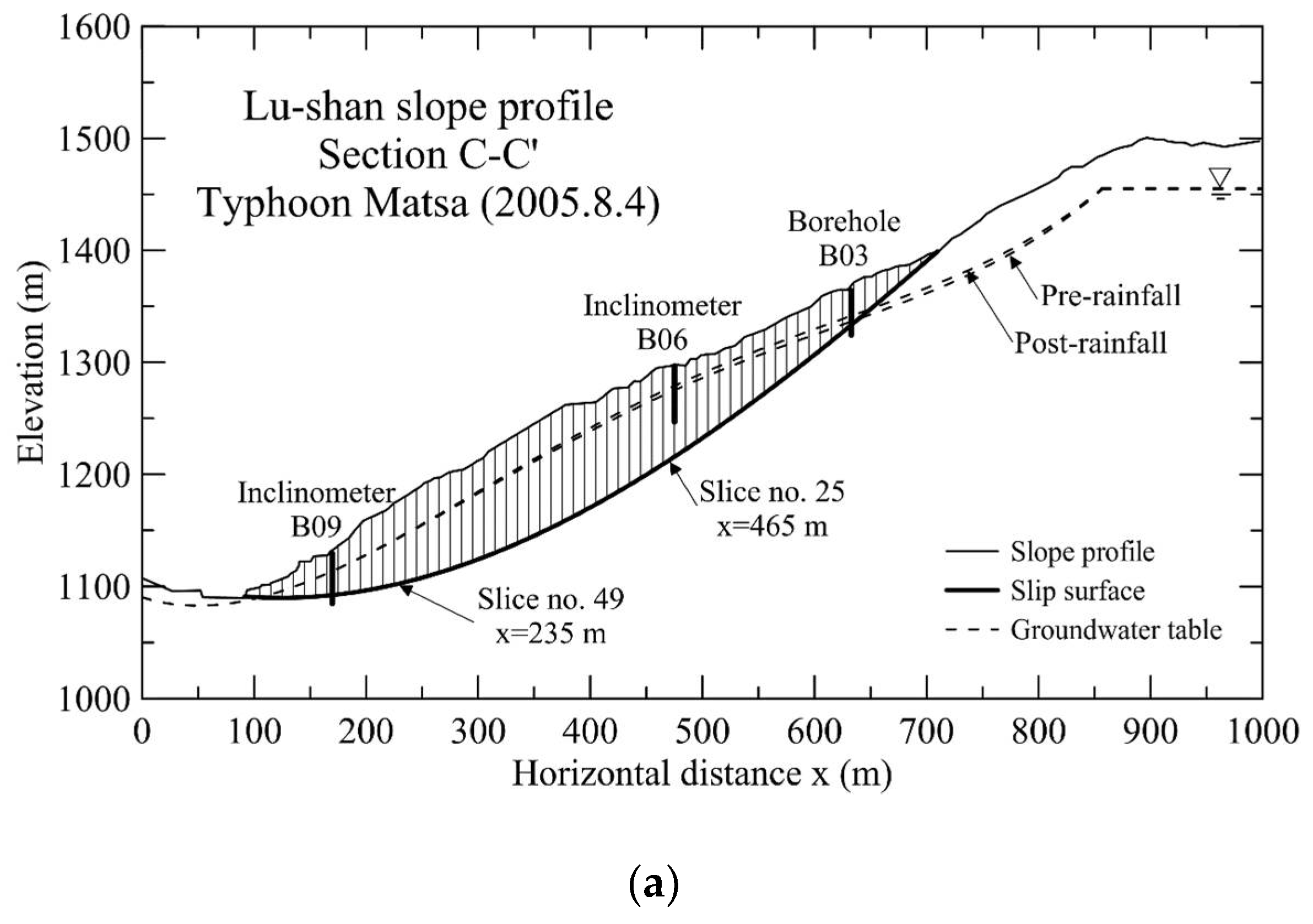
The studied slope is located between km markers 44 and 91 along Provincial Highway 14, which winds through a landslide-prone area (Figure 12). The sliding mass has maximum width, length and depth of 480 m, 820 m and 100 m, respectively, which spans over a height of about 400 m (between elevations of 1085 and 1500 m above sea level) and covers an area of about 30 ha. In situ borehole logging, in situ testing, laboratory testing, and groundwater table measurements were conducted during the monitoring period. The major rock formation in this area is slate (SL) with intensive joints and is covered by alluvium deposits with depths of a few centimeters to tens of meters. Cross-section C-C’ is approximately in the direction of landslides, along which boreholes B01, B03, B06 and B09 were drilled. Groundwater tables were measured at boreholes B03, B06 and B09 using electronic groundwater pressure sensors. Slope displacements were measured at borehole B09 using an in-hole inclinometer. Slope displacements at boreholes B03 and B06 were based on Global Positioning System (GPS) data obtained at stations B21 and A25, respectively, which are located in the vicinity of the boreholes.
Figure 13 shows cross-section C-C’ with a detected failure surface (bold solid line). The failure surface reported by Huang et al. [11] is also plotted (dotted line). In the present study, a new failure surface based on time-domain reflectometry (TDR, as shown in Figure 13) and GPS data is drawn; this surface was not considered in the study of Huang et al. [11]. The slip surface is located approximately at the interface of colluviums and highly fractured (or weathered) slate strata with a maximum depth of about 100 m, associated with rock quality designation (RQD) values distributed over a wide range. Deriving the material properties using an undisturbed sampling technique for such a depth is costly and time-consuming. Figure 13 shows the cross-section C-C’ of the Lu-Shan slope with a deep-seated slip surface approximately along the interface of colluvium and heavily weathered slate (SL) inter-layered with sandy slate (SSL), as shown in the cross-section. An example of the rock quality designation (RQD) profile obtained from borehole B09 is also shown in Figure 13. The slip surface shown in Figure 13 is identical with that reported in a monitoring and remediation project supervised by the governmental authority [17].
Figure 14 shows the daily rainfall recorded at an on-site weather station during the period of July 2005 to May 2006. Several peaks of daily rainfall caused by typhoons can be seen. Major events of intensive rainfall are mostly induced by typhoons. These rainfall events and the observed post-rainfall slope displacements are summarized in Table 3.
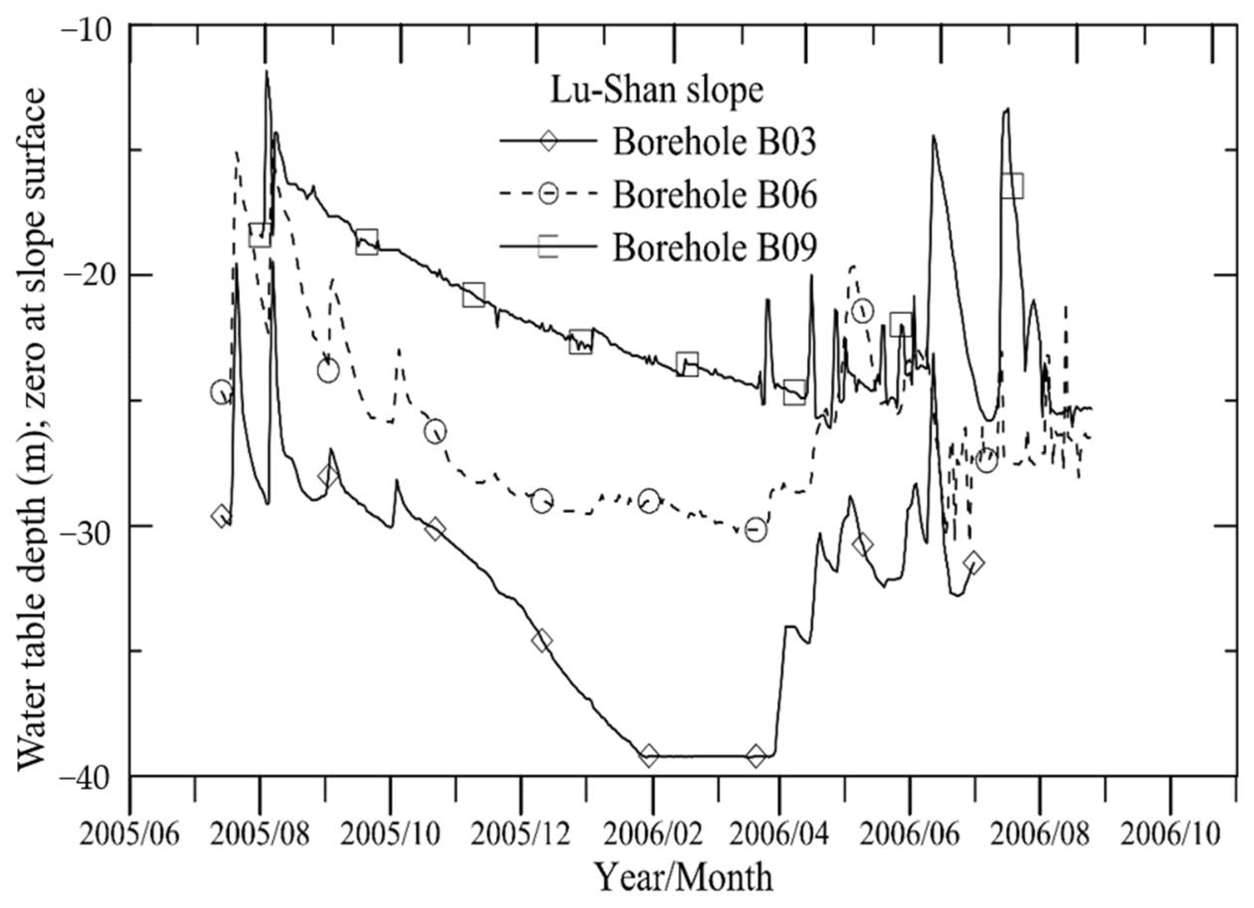
Figure 15 shows a comparison of the measured groundwater table heights at various locations of the failure mass. It can be seen that all groundwater tables respond to the rainfall event with abrupt rises at the central (borehole B06) and near-top (borehole B03) parts of the slope. The groundwater table heights near the toe of the slope (borehole B09) were a higher level than those measured at the upper portions of the slope (boreholes B03 and B06), suggesting that a perched water table exists around the toe of the slope, undermining the stability of the slope.
Figure 16 compares the measured displacements at various locations of the sliding mass. For most of the rainfall events, measured slope displacements at various locations are similar, except those for the last rainfall event. For the last event of rainfall (or slope movements), the displacements at the upper portions (boreholes B03 and B06) were greater than those around the toe (borehole B09), suggesting that a displacement field with a decreasing shear displacement toward the toe of the slope (see Figure 9a,b) is applicable here. This pattern of displacements also suggests that a volumetric contraction occurred within the sliding mass, which acted as a buffer in transmitting lateral thrust from the upper portion of the sliding mass.
Figure 17 shows variations of Fs (Equation (20)) calculated based on the groundwater tables measured after rainfall events nos. 1–8. In this analysis, cohesion intercept (c) = 65 kPa and φ = 32° were used based on the hypothesis that the slope attained the critical condition (Fs = 1.0) during rainfall event no. 1 with a high groundwater table. The value of c = 65 kPa was determined based on the following empirical equation [30,31]:
where
- c: cohesion intercept (kPa)
- z: depth (m).
The average depth of the slip surface z ≒ 65 m (Figure 13), resulting in c = 65 kPa in the analysis. Note that an arbitrary value of c can be used to derive a calibrated value of φ based on the measured groundwater table height in event no. 1. The essence of the proposed procedure is that accurate predicted slope displacements for subsequent rainfall events (event nos. 2–8) can be obtained regardless of the c value used (to be explained in Figure 18). It can be seen in Figure 17 that values of Fs decrease rapidly during each rainfall event. An increasing trend of Fs in response to decreasing heights of the groundwater table during the period August 2005 to April 2006 can also be seen. In general, the increasing Fs corresponded to the trend of decreasing groundwater table heights during event nos. 1 to 4. However, this increasing trend of Fs (from event nos. 1 to 4) contradicts to the trend of slope displacements (see Figure 13). Therefore, an immediate rainfall-induced groundwater table rise may have a dominant influence on slope movement (and cumulative slope displacement). The influence of a long-term descending groundwater table on (cumulative) slope movement is insignificant. A misleading conclusion may be obtained if only values of Fs are used for slope stability evaluations.
4. Results and Discussion
4.1. Results of Back-Analysis
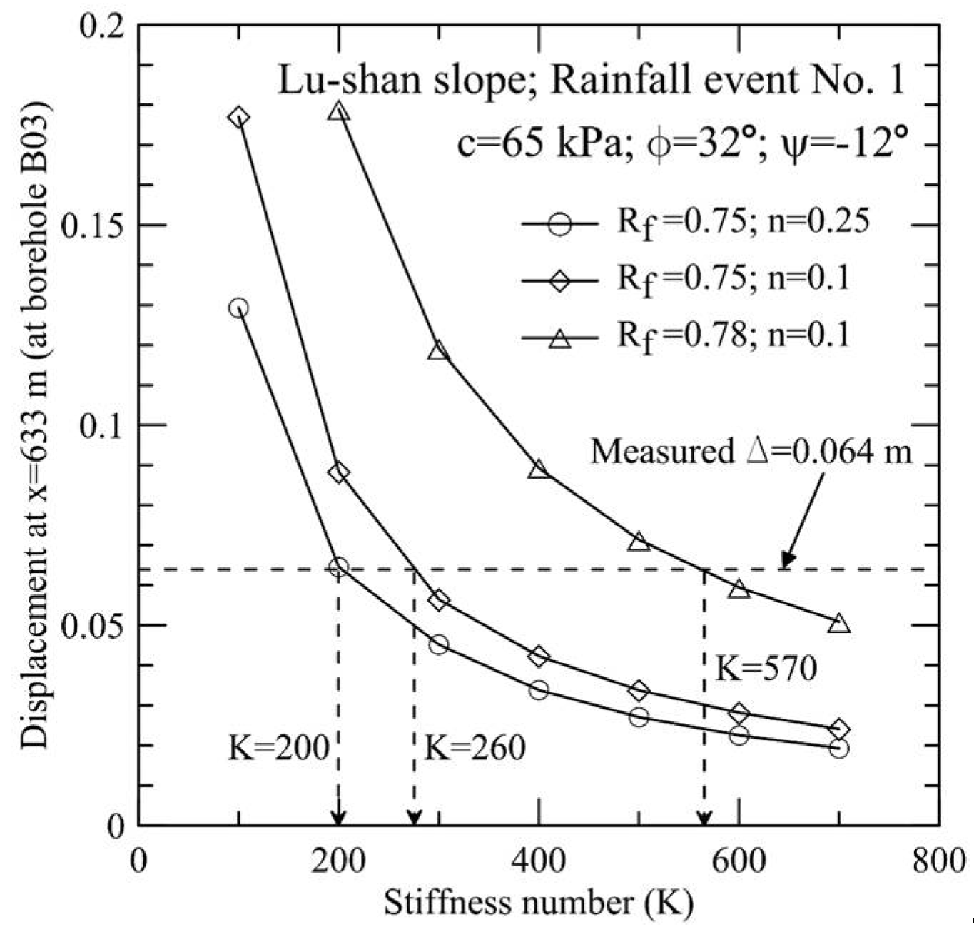
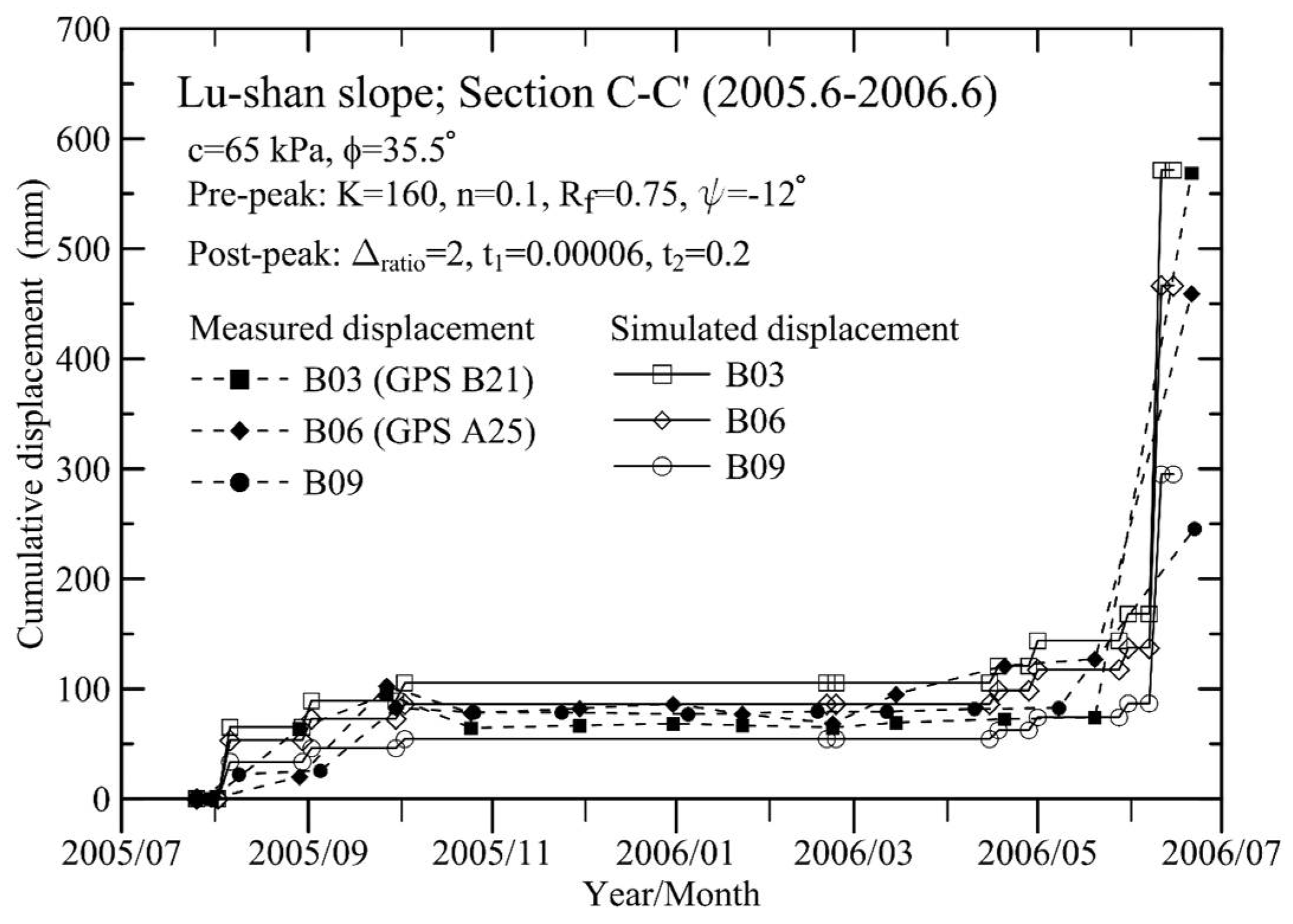
Figure 18 shows the results of a parametric study of the Fs vs. φ relationship for various values of c (=0 and 65 kPa) and Δφ (=0°, 1°, 3°, and 5°) using Janbu’s method of slices. The value of Δφ is changed to investigate its effect (or that of the curvature of the M-C failure envelope) on the value of Fs. The condition of Δφ = 0° is a special case of a linear M-C failure envelope. Figure 18 also shows that different values of Δφ result in different values of φ that generate Fs = 1.0. These back-calculated values of φ are used in the following analyses. Figure 19 shows the result of a back-analysis for displacement-related parameters (K, Rf, and n in Equations (1)–(4) and (6)), obtained using c = 65 kPa, φ = 32° and Ψ = 0°. The use of Ψ = 0° is based on the assumption that the slope is in a large displacement state before the occurrence of rainfall event no. 1 on 4 August 2005. This assumption is not necessarily true; other assumptions are investigated later. In practice, an infinite number of curves of the Δi (x = 633 m) vs. K relationship, as shown in Figure 19, can be used. However, only three typical curves are shown in Figure 19 for simplicity. It can be seen that these curves, which use various values of Rf and n, yield different back-calculated values of K that meet the requirement of Δi (at x = 633 m) = 0.064 m. The strength parameters, c = 65 kPa, φ = 32° and Ψ = 0°, obtained in Figure 18 and the displacement parameters, Rf = 0.75, n = 0.1 and K = 200, obtained in Figure 19 are used to calculate the incremental displacements in rainfall events 2–8. The curves of cumulative displacements for all rainfall events are shown in Figure 20a,c. These calculated curves of slope displacements agree well with the measured ones in the following manner: (1) The calculated cumulative displacements are comparable to the observed long-term displacements; (2) The use of Ψ = −12° for constructing the displacement field results in calculated displacements that well agree with the slope displacements observed at various locations; (3) Three sets of K, n, and Rf generate similar cumulative slope displacement curves.
4.2. Influence of Post-Peak Softening on Slope Displacements
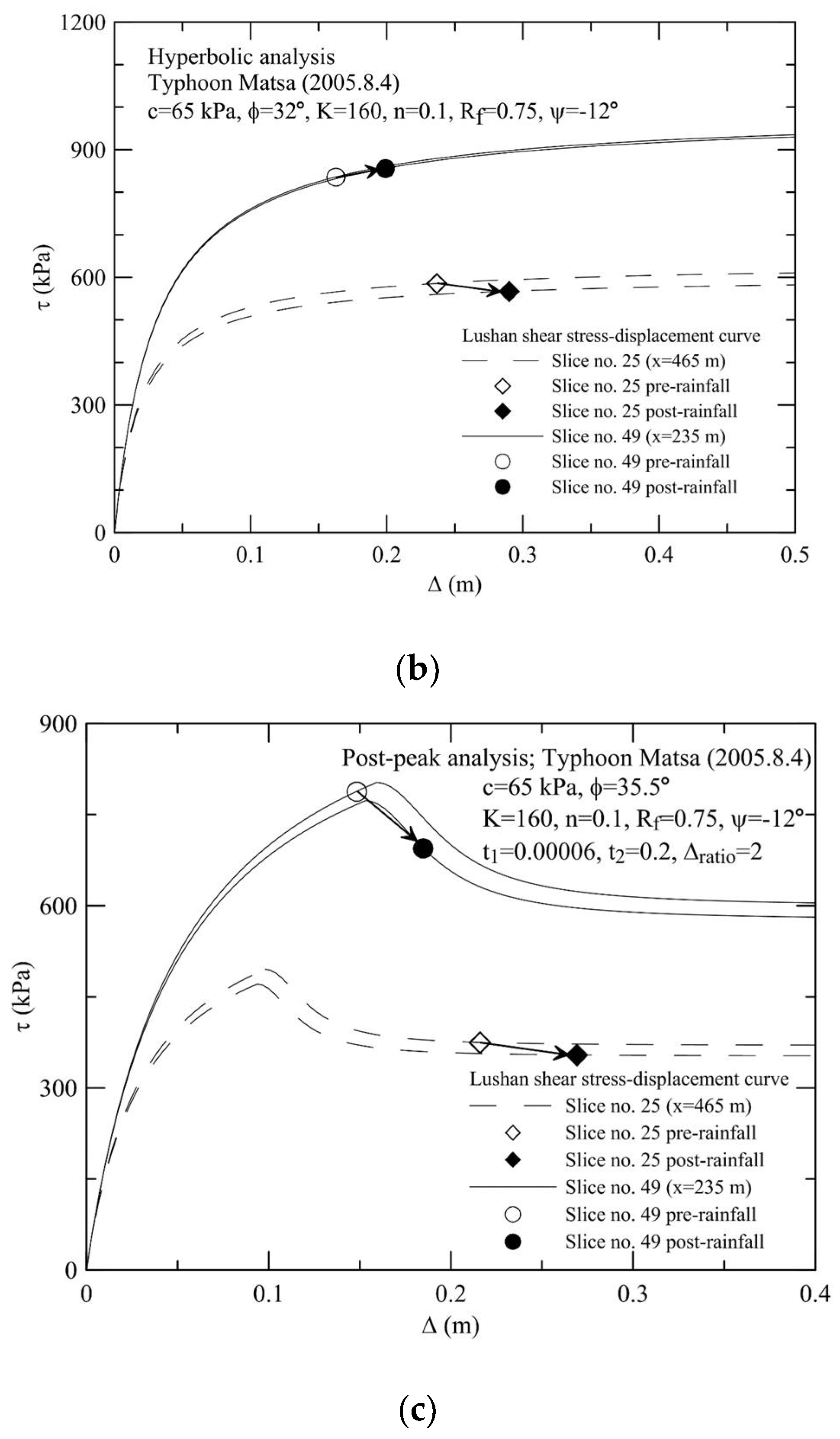
To consider post-peak softening behavior in the displacement analysis using FFDM, a back-analysis for the displacement parameter K based on rainfall event no. 1 similar to that performed in Figure 19 is shown in Figure 21. Note that infinite sets of parameters (c, φ), Ψ, (t1, t2, Δratio) and (K, n, Rf) can be used to the requirement of calculated Δi (at x = 633 m) = 0.064 m. For simplicity, only three typical curves are shown. For c = 65 kPa, φ = 35.5°, Ψ = 12°, t1 = 0.0006, t2 = 0.2, Δratio = 2, n = 0.1, 0.25, Rf = 0.75, 0.78 and three values of K (=145, 160, and 185) can be used to satisfy Δi = 0.064 m. Figure 22 shows the results of displacement calculations that take into account post-peak softening of the slope material. A comparison of Figure 22 with Figure 20a–c reveals that post-peak softening has a remarkable influence on the calculated slope displacements for event no. 8, for which relatively large displacements were measured. The mechanism of post-peak softening was further investigated using the parameter set shown in Figure 22. The stress-displacement behavior at the base of slice no. 25 (central portion of the slope) and slice no. 49 (near the slope toe) was considered, as shown in Figure 23a. Figure 23b shows the stress-displacement curves corresponding to pre-rainfall and post-rainfall stress states at the base of slice nos. 25 and 49 obtained without consideration of post-peak softening. The arrows in this figure show the transition of stress (and displacement) states from pre-rainfall to post-rainfall states. It can be seen that the soil at slice no. 25 (upper portion of the slope) is under the state of stress hardening due to the limitation of using a hyperbolic stress-displacement relationship. To take into account the influence of post-peak softening behavior of geomaterials on the rainfall-induced slope displacements, typical values of post-peak softening parameters obtained in Figure 4b and Figure 5, namely, t1 = 0.00006, t2 = 0.2 and Δratio = 2, are used in the FFDM analyses. The results shown in Figure 23c suggest that the soil at the base of slice no. 25 undergoes a transition from a pre-peak state to a post-peak state during rainfall event no. 1, which was not found in previous analyses.
5. Conclusions
A natural slope subjected to recurrent rainfall-induced movements was studied using FFDM. In addition to the use of a hyperbolic model of the shear stress vs. shear displacement relationship and an improved displacement compatibility function, curved M-C failure envelopes and post-peak strength softening were taken into account in the slope displacement analyses. The results of the case study showed that:
- (1)
- The accuracy of slope displacement predictions was not influenced by the curvature of the M-C failure envelope used in the back-analyses and displacement analyses.
- (2)
- Post-peak soil strength softening was successfully described by the proposed stress-displacement relationship model. New parameters, including normalized post-peak strength deterioration (t) and residual displacement ratio (Δratio), were studied using direct shear tests on various soil types. Good agreements between the experimental and simulated post-peak stress vs. displacement relationships were obtained.
- (3)
- The accuracy of the slope displacement computations can be improved by incorporating the post-peak stress-displacement relationship in the analysis. The results of a case study on the Lu-Shan slope revealed that a transition from pre-peak to post-peak states for the slip surface near the slope toe may have taken place during the first rainfall event in the monitoring period. This critical feature may be overlooked when post-peak strength deterioration is not taken into account in the displacement analysis.
Author Contributions
C.-L.L. contributed to the conception, formal analysis, investigation, data curation, writing—review and editing of the study; C.-C.H. contributed to the methodology, validation, project administration, funding acquisition. All authors have read and agreed to the published version of the manuscript.
Funding
This study was supported by the Ministry of Science and Technology, Taiwan, under research grant [MOST 104-2221-E-006-MY3].
Data Availability Statement
The data presented in this study are available on request from the corresponding author.
Conflicts of Interest
The authors declare no conflict of interest.
References
- Huang, C.-C. Caussian-distribution-based hyetographs and their relationships with debris flow initiation. J. Hydrol. 2011, 41, 251–265. [Google Scholar] [CrossRef]
- Huang, C.-C. Critical rainfall for typhoon-induced debris flows in the Western Foothills, Taiwan. Geomorphology 2013, 185, 87–95. [Google Scholar] [CrossRef]
- Huang, C.-C.; Lo, C.-L. Simulation of subsurface flows associated with rainfall-induced shallow slope failures. J. GeoEng. 2013, 8, 101–111. [Google Scholar]
- Yu, G.; Zhang, M.; Cong, K.; Pei, L. Critical rainfall thresholds for debris flows in Sanyanyu, Zhouqu County, Gansu Province, China. Q. J. Eng. Geol. Hydrogeol. 2015, 48, 224–233. [Google Scholar] [CrossRef]
- Tu, G.; Huang, R. Infiltration in two types of embankments and the effects of rainfall time on the stability of slopes. Q. J. Eng. Hydrogeol. 2016, 49, 286–297. [Google Scholar] [CrossRef]
- Burland, J.B. On the compressibility and shear strength of natural clays. Rankine Lecture. Geotechnique 1990, 40, 329–378. [Google Scholar] [CrossRef]
- Huang, C.-C.; Tatsuoka, F. Stability analysis for footings on reinforced sandy slopes. Soils Found. 1994, 34, 21–37. [Google Scholar] [CrossRef] [Green Version]
- Leshchinsky, B.; Ambauen, S. Limit equilibrium and limit analysis: Comparison of benchmark slope stability problems. J. Geotech. Geoenviron. Eng. 2016, 141, 04015043. [Google Scholar] [CrossRef]
- Yin, Y.; Huang, B.; Wang, W.; Wei, Y.; Ma, X.; Zhao, C. Reservoir-induced landslides and risk control in Three Gorges project on Yangtze river, China. J. Rock Mech. Geotech. Eng. 2016, 8, 577–595. [Google Scholar] [CrossRef] [Green Version]
- Huang, C.-C. Developing a new slice method for slope displacement analyses. Eng. Geol. 2013, 157, 39–47. [Google Scholar] [CrossRef]
- Huang, C.-C.; Yeh, S.-W. Predicting periodic rainfall-induced slope displacements using force-equilibrium-based finite displacement method. J. GeoEng. 2015, 10, 83–89. [Google Scholar]
- Kondner, R.L. Hyperbolic stress-strain response: Cohesive soils. J. Soil Mech. Found. Div. 1963, 89, 115–144. [Google Scholar] [CrossRef]
- Duncan, J.M.; Chang, C.-Y. Nonlinear analysis of stress and strain in soil. J. Soil Mech. Found. Div. Proc. 1970, 96, 1629–1653. [Google Scholar] [CrossRef]
- Tatsuoka, F.; Siddiquee, M.S.A.; Park, C.-C.; Sakamoto, M.; Abe, F. Modelling stress-strain relations of sand. Soils Found. 1993, 33, 60–81. [Google Scholar] [CrossRef] [Green Version]
- Mesri, G.; Huvaj-Sarihan, N. Residual shear strength measured by laboratory tests and mobilized in landslides. J. Geotech. Geoenviron. Eng. 2012, 138, 585–593. [Google Scholar] [CrossRef] [Green Version]
- Eid, H.; Rabie, K. Fully softened shear strength for soil slope stability analyses. Int. J. Geomech. 2017, 17, 04016023. [Google Scholar] [CrossRef]
- Huang, C.-C. Back-calculating strength parameters and predicting displacements of deep-seated sliding surface comprising weathered rocks. Int. J. Rock Mech. Min. Sci. 2016, 88, 98–104. [Google Scholar] [CrossRef]
- Wu, K.-W. Applying Results of True Direct Shear Tests to the Stability Analysis for Integrated Road-Dyke Structures. Master’s Thesis, Feng-Chia University, Taichung City, Taiwan, 2011. (In Chinese). [Google Scholar]
- Hsu, H.-Y. Modeling on the Behavior of Soils Subjected to Cyclic Direct Shear. Master’s Thesis, National Cheng Kung University, Tainan City, Taiwan, 2017. (In Chinese). [Google Scholar]
- Hoek, E.; Brown, E.T. Empirical strength criterion for rock masses. J. Geotech. Eng. Div. ASCE 1980, 106, 1013–1035. [Google Scholar] [CrossRef]
- Duncan, J.M.; Wright, S.G. Soil Strength and Slope Stability; Wiley: Ney York, NY, USA, 2005. [Google Scholar]
- Lienhard, J.H. The Engines of Our Ingenuty: An Engineer Looks at Technology and Culture; Oxford University Press: Oxford, UK, 2003; p. 272. [Google Scholar]
- Chu, B.-L.; Huang, C.-R.; Jeng, S.-Y. Study on Terrace Sedimentary and Tou-ka-san Gravelly Strata Using In-Situ Direct Shear Tests. In Proceedings of the 3rd National Geotechnical Conference, Taichung City, Taiwan, 11–13 September 1989; pp. 695–706. [Google Scholar]
- Davoudi, M.H. Influence of willow root density on shear resistance paramters in fine grain soils using in situ direct shear tests. Res. J. Environ. Sci. 2011, 5, 157–170. [Google Scholar]
- Qiu, J.-Y.; Tatsuoka, F.; Uchimura, T. Constant pressure and constant volume direct shear tests on reinforced sand. Soils Found. 2000, 40, 1–17. [Google Scholar] [CrossRef] [Green Version]
- Hsu, C. Influences of the Slit Size on the Direct Shear Strength of Gravelly Soils. In Proceedings of the National Conference on Rock Engineering, Tainan City, Taiwan, 26 June 2006; pp. 31–40. [Google Scholar]
- Hsu, W. Simulating Physical Properties of Gravelly Strata Using Three-Dimensional Discrete Element Method. Master’s Thesis, Chaoyang University of Technology, Taichung City, Taiwan, 2009. (In Chinese). [Google Scholar]
- Ziaie Moayed, R.; Alibolandi, M.; Alizadeh, A. Specimen size effects on direct shear test of silty sands. Int. J. Geotech. Eng. 2017, 11, 198–205. [Google Scholar] [CrossRef]
- Janbu, N. Slope Stability Computations. Embankment-Dam Engineering; Hirschfeld, R.C., Poulos, S.J., Eds.; John Wiley & Sons: Hoboken, NJ, USA, 1973; pp. 47–86. [Google Scholar]
- Japanese Highway Association. Guidelines for Cut Slopes and Slope Stabilization Engineering; Japanese Highway Association: Tokyo, Japan, 1986. (In Japanese) [Google Scholar]
- Japanese Geotechnical Society. Strength Parameters in Design—c, φ and N values. Soil Foudnation Eng. Libr. 1988, 32, 127. (In Japanese) [Google Scholar]
Figure 1.
Schematic of hyperbolic curve.
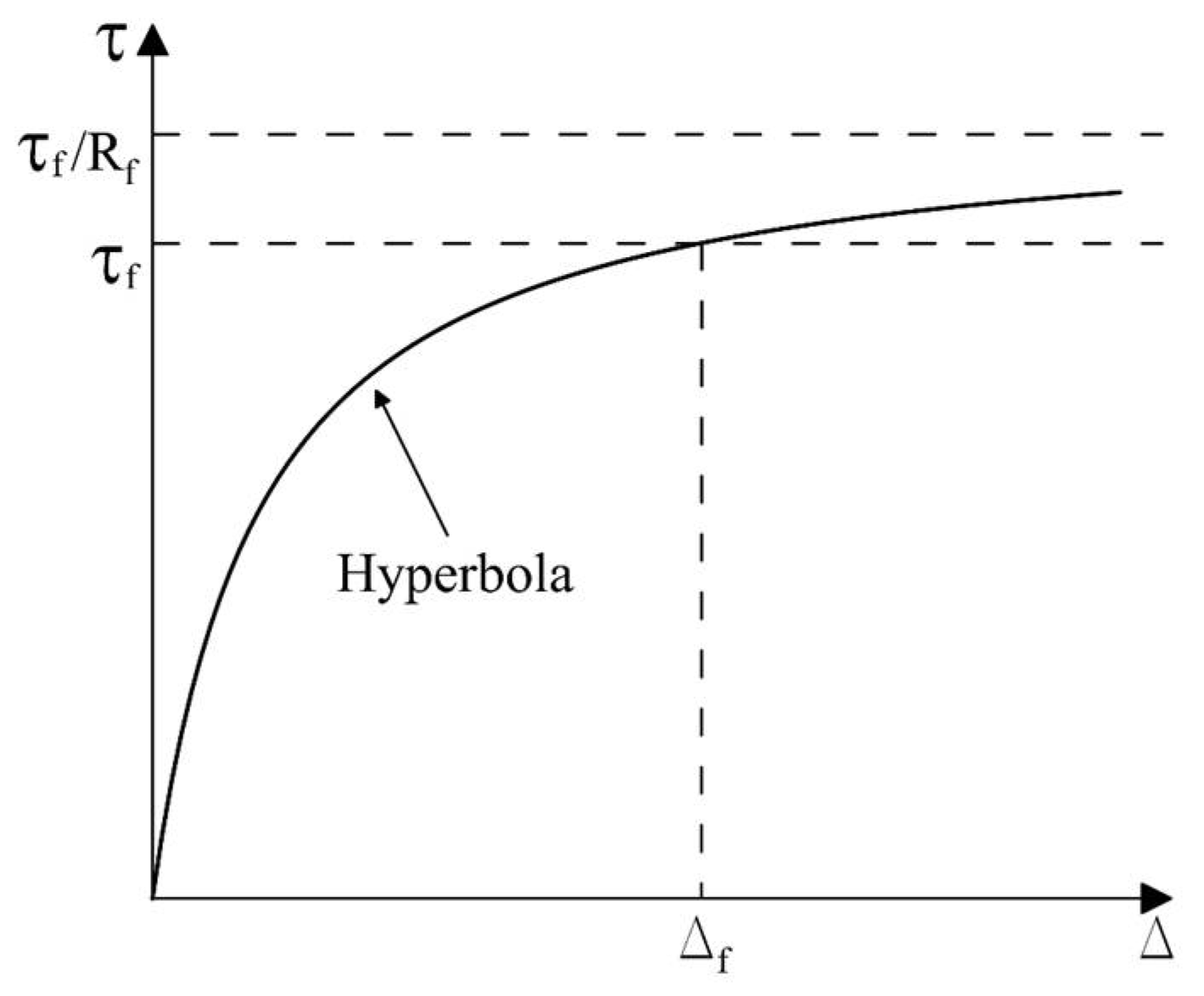
Figure 2.
Coordinate system for pre-peak and post-peak curves.
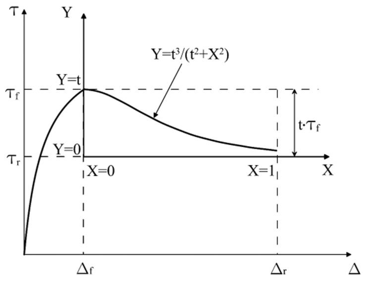
Figure 4.
(a) Experimental and fitted lines for t vs. σn relationship obtained in various studies; (b) Close-up of t vs. σn relationship reported by Wu (2011) and Hsu (2017).
Figure 4.
(a) Experimental and fitted lines for t vs. σn relationship obtained in various studies; (b) Close-up of t vs. σn relationship reported by Wu (2011) and Hsu (2017).

Figure 6.
Comparison of calculated and experimental stress-displacement curves reported by Wu (2011).
Figure 6.
Comparison of calculated and experimental stress-displacement curves reported by Wu (2011).
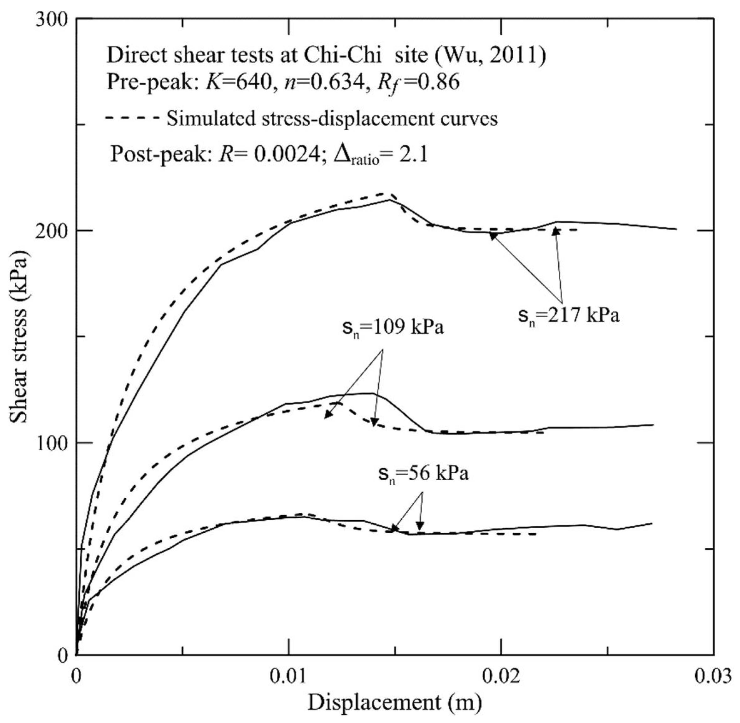
Figure 7.
Comparison of calculated and experimental stress-displacement curves reported by Hsu (2017).
Figure 7.
Comparison of calculated and experimental stress-displacement curves reported by Hsu (2017).
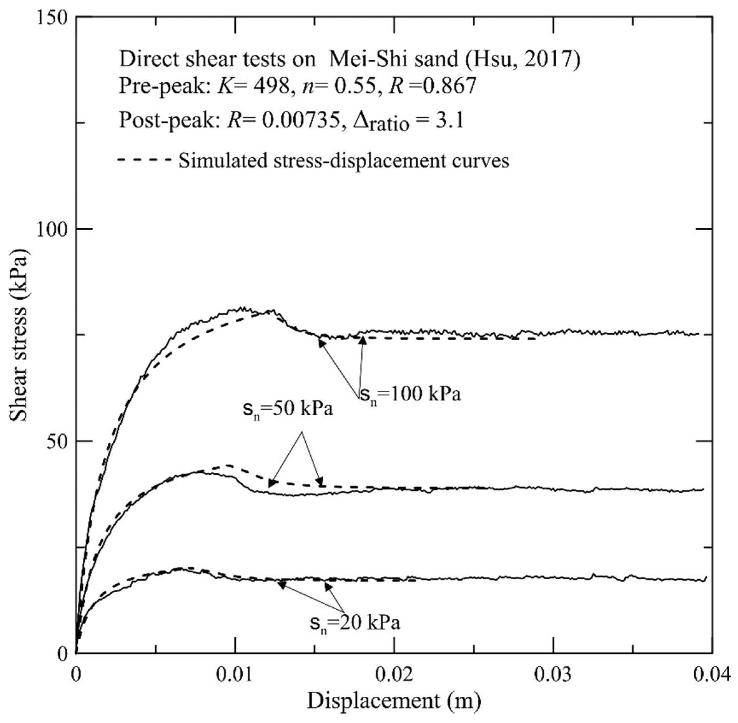
Figure 9.
(a) Vector of displacements along failure surface and inter-slice faces for ψ < 0 and (b) Hodogram for ψ < 0.
Figure 9.
(a) Vector of displacements along failure surface and inter-slice faces for ψ < 0 and (b) Hodogram for ψ < 0.

Figure 10.
(a) Vector of displacements along failure surface and inter-slice faces for ψ = 0 and (b) Hodogram for ψ = 0.
Figure 10.
(a) Vector of displacements along failure surface and inter-slice faces for ψ = 0 and (b) Hodogram for ψ = 0.

Figure 12.
Locations and plan view of studied slope.
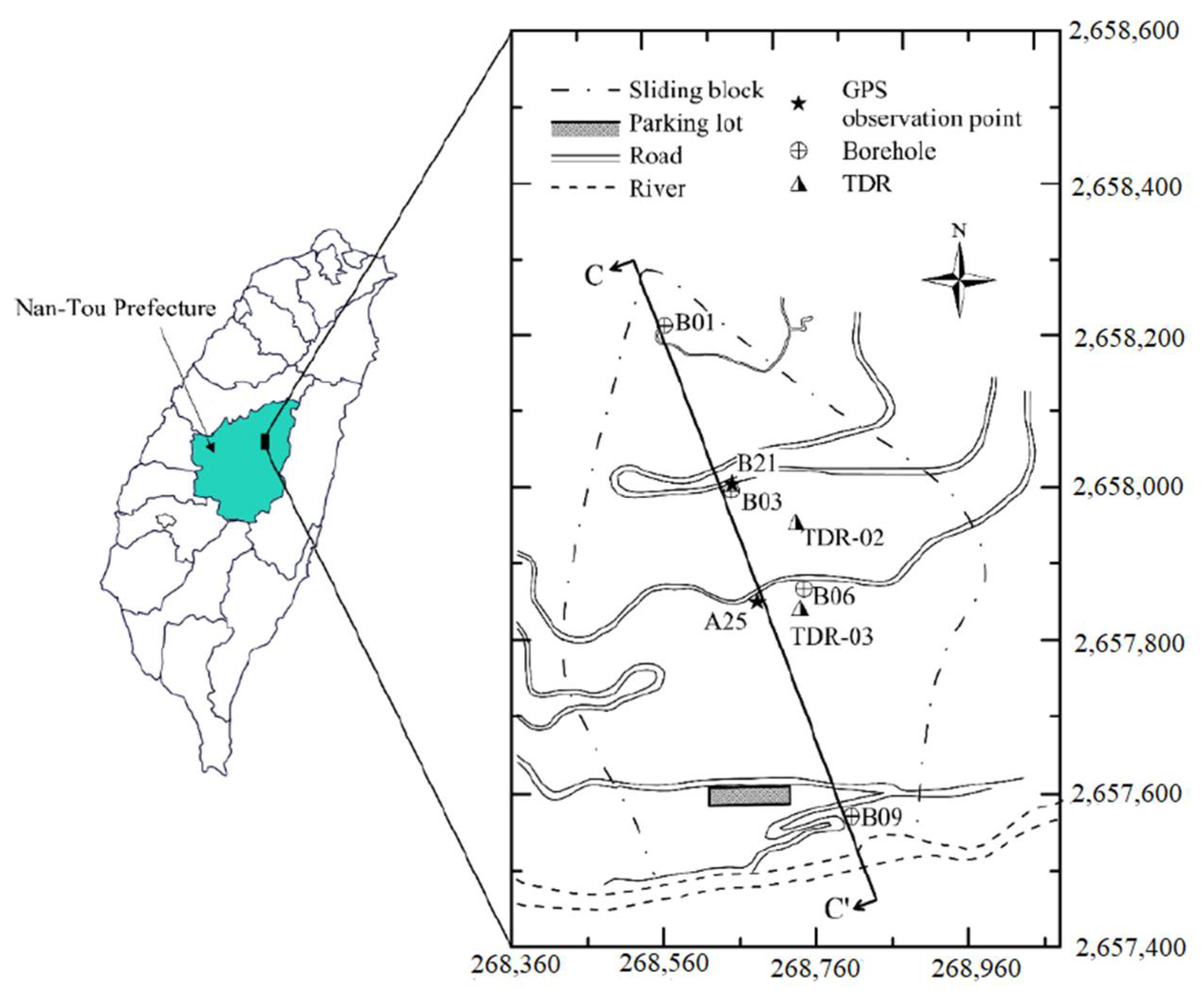
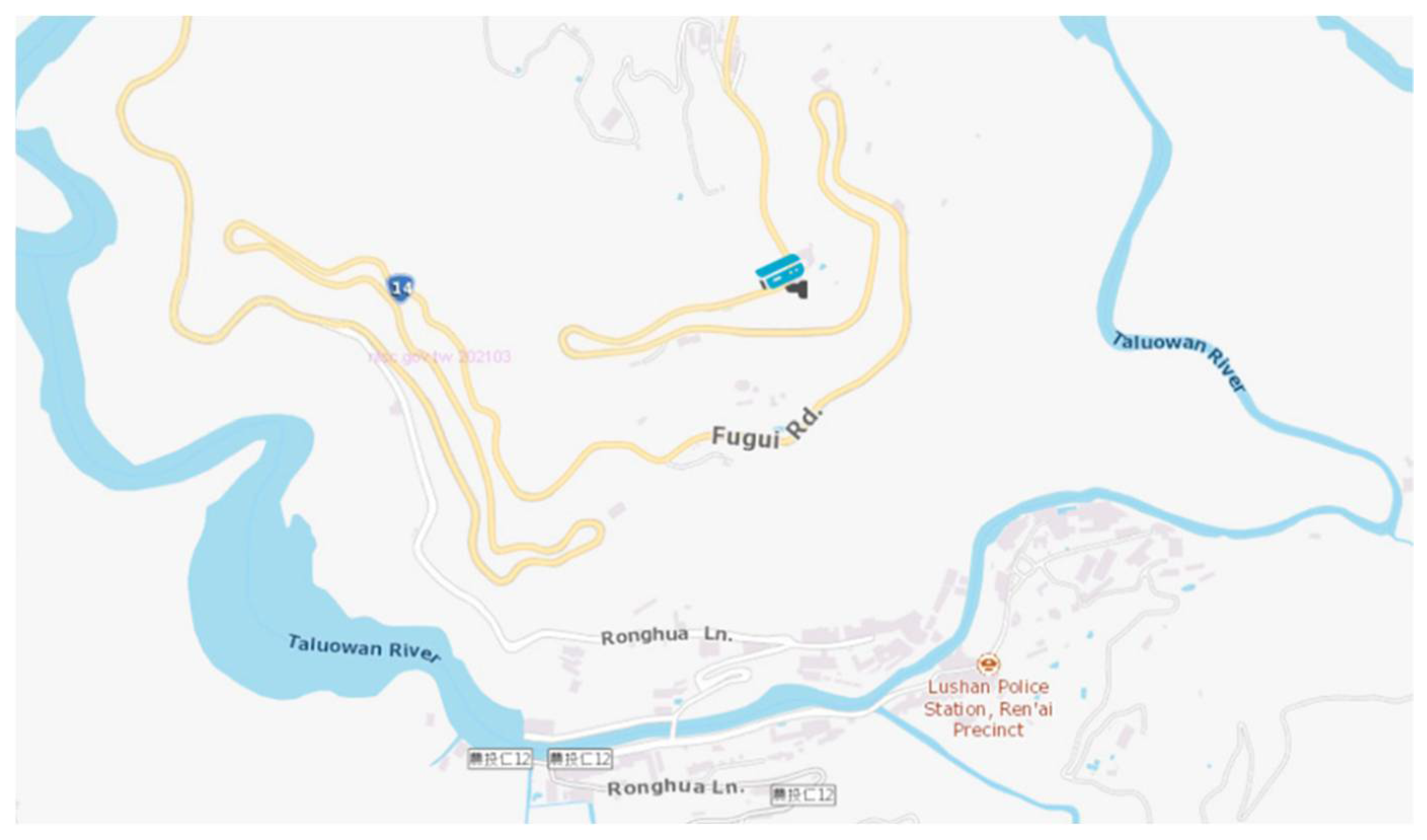
Figure 13.
Cross-section of studied slope.

Figure 14.
Records of daily rainfall, groundwater levels, and cumulative slope displacements.
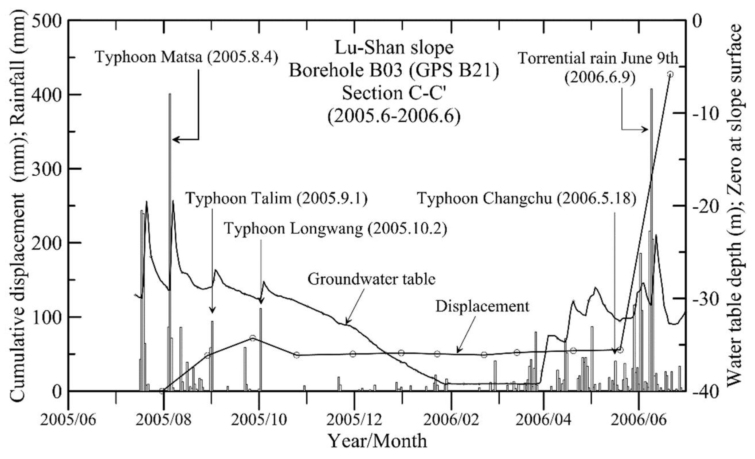
Figure 15.
Comparison of groundwater table heights measured at various boreholes.

Figure 16.
Comparison of cumulative slope displacements measured at various boreholes.
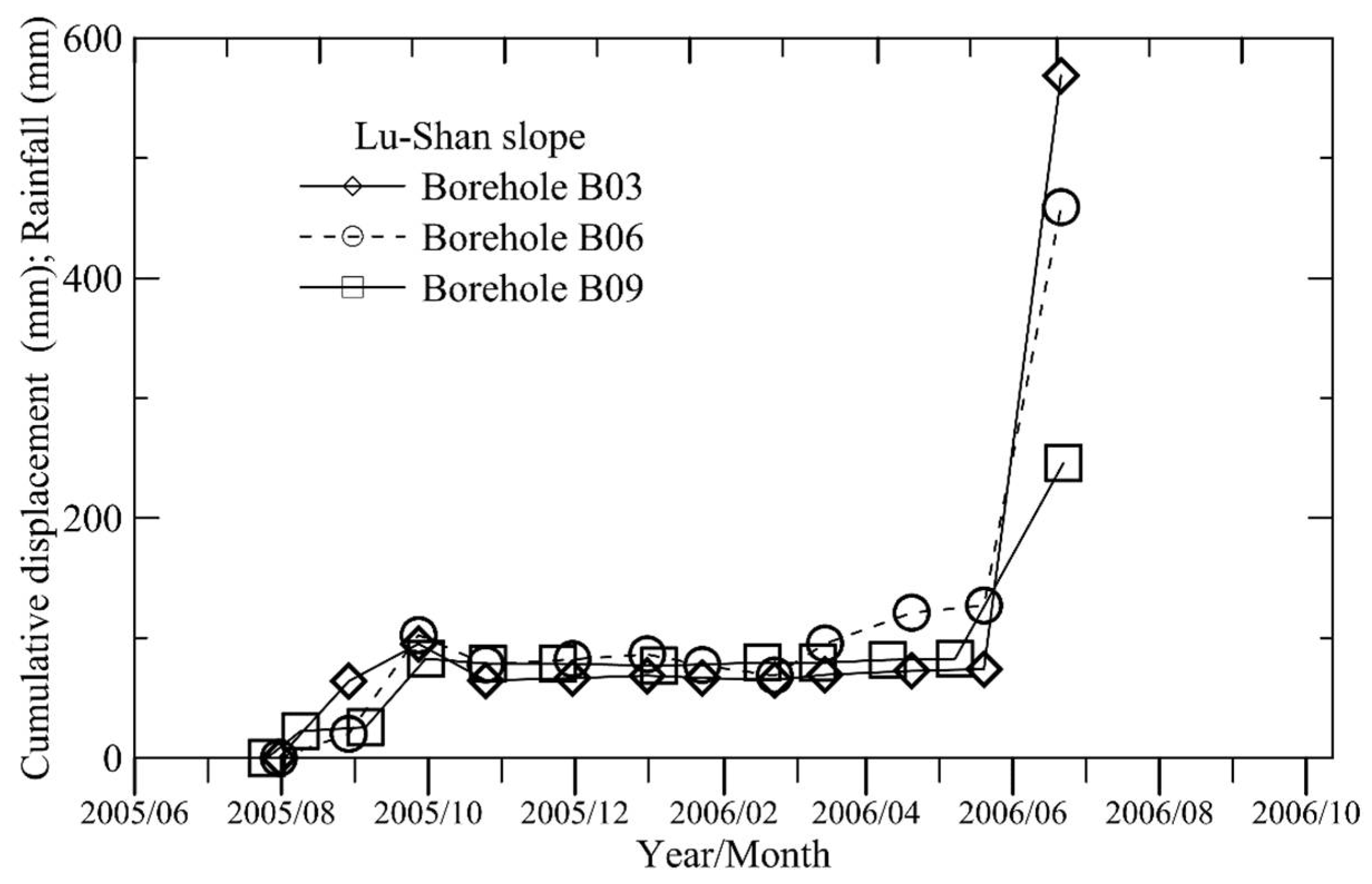
Figure 17.
Comparison of recorded groundwater table heights and calculated safety factors for studied slope.
Figure 17.
Comparison of recorded groundwater table heights and calculated safety factors for studied slope.

Figure 18.
Results of back-analyses for stress-related parameter φ obtained using various values of Rf and n.
Figure 18.
Results of back-analyses for stress-related parameter φ obtained using various values of Rf and n.
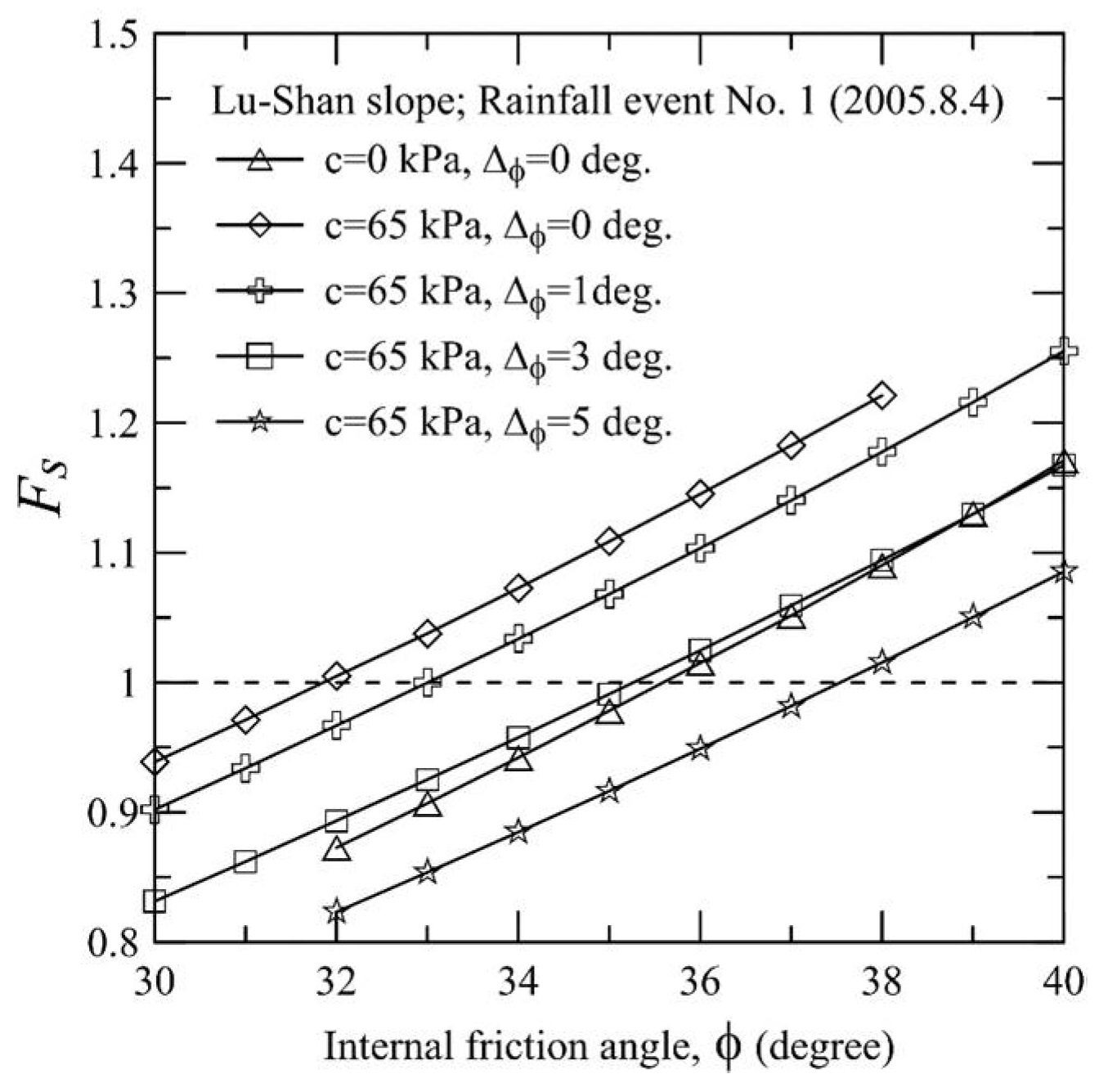
Figure 19.
Results of back-analyses for displacement-related parameter K various values of c and Δφ.
Figure 19.
Results of back-analyses for displacement-related parameter K various values of c and Δφ.

Figure 20.
Comparison between measured slope displacements and those calculated using (a) c = 65 kPa, φ = 3 2°, K = 260, n = 0.1, Rf = 0.75 and ψ = −12°; (b) c = 65 kPa, φ = 32°, K = 200, n = 0.25, Rf = 0.75 and ψ = −12°; (c) c = 65 kPa, φ = 32°, K = 570, n = 0.1, Rf = 0.78 and ψ = −12°.
Figure 20.
Comparison between measured slope displacements and those calculated using (a) c = 65 kPa, φ = 3 2°, K = 260, n = 0.1, Rf = 0.75 and ψ = −12°; (b) c = 65 kPa, φ = 32°, K = 200, n = 0.25, Rf = 0.75 and ψ = −12°; (c) c = 65 kPa, φ = 32°, K = 570, n = 0.1, Rf = 0.78 and ψ = −12°.


Figure 21.
Results of back-analyses for displacement-related parameter K obtained using various values of Rf and n as well as considering post-peak softening behavior.
Figure 21.
Results of back-analyses for displacement-related parameter K obtained using various values of Rf and n as well as considering post-peak softening behavior.
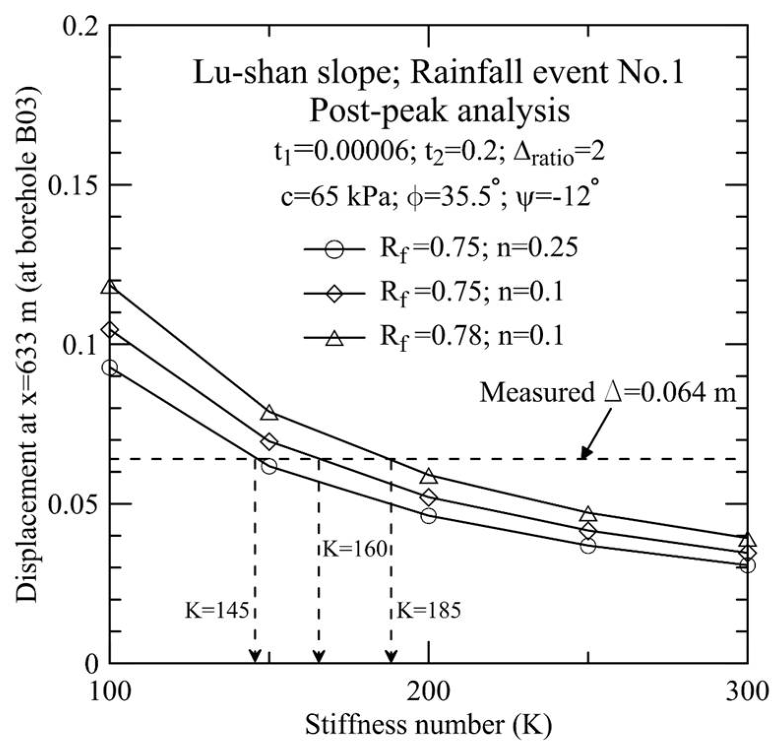
Figure 22.
Comparison between slope displacements measured at various locations and those calculated using c = 65 kPa, φ = 35.5°, K = 160, n = 0.1, Rf = 0.75 and ψ = −12° as well as taking into account post-peak soil strength softening.
Figure 22.
Comparison between slope displacements measured at various locations and those calculated using c = 65 kPa, φ = 35.5°, K = 160, n = 0.1, Rf = 0.75 and ψ = −12° as well as taking into account post-peak soil strength softening.

Figure 23.
(a) Results of detailed stress analyses for slice nos. 25 and 49 of studied slope; (b) Variations of pre- and post-rainfall shear stresses obtained (b) with and (c) without consideration of post-peak softening of soils.
Figure 23.
(a) Results of detailed stress analyses for slice nos. 25 and 49 of studied slope; (b) Variations of pre- and post-rainfall shear stresses obtained (b) with and (c) without consideration of post-peak softening of soils.


Table 1.
Input parameters used for simulating stress-displacement curves reported by Wu (2011).
| σn (kPa) | a | b | K | n | Rf | Measured | Simulated | ||
|---|---|---|---|---|---|---|---|---|---|
| Δratio | t | Δratio | t | ||||||
| 56 | 2.3 × 10⁻⁵ | 0.013 | 640 | 0.634 | 0.86 | 2 | 0.121 | 1.97 | 0.142 |
| 109 | 1.5 × 10⁻⁵ | 0.007 | 1.8 | 0.155 | 1.844 | 0.122 | |||
| 217 | 9.5 × 10⁻⁶ | 0.004 | 1.6 | 0.073 | 1.586 | 0.082 | |||
Table 2.
Input parameters used for simulating stress-displacement curves reported by Hsu (2017).
| σn (kPa) | a | b | K | n | Rf | Measured | Simulated | |||
|---|---|---|---|---|---|---|---|---|---|---|
| Δratio | t | Δratio | t | |||||||
| 20 | 4.8 × 10⁻⁵ | 0.043 | 498 | 0.55 | 0.867 | 3 | 0.165 | 2.97 | 0.149 | |
| 50 | 2.9 × 10⁻⁵ | 0.0196 | 2.7 | 0.098 | 2.74 | 0.123 | ||||
| 100 | 2.0 × 10⁻⁶ | 0.0108 | 2.4 | 0.088 | 2.38 | 0.078 | ||||
Table 3.
Events of intensive rainfall and measured slope displacements.
| Location of Bore Hole Rainfall Event | Measured Cumulative Displacement (mm) | ||
|---|---|---|---|
| B03 x = 633 m | B06 x = 475 m | B09 x = 170 m | |
| Event no. 1 (4 August 2005, Typhoon Matsa) | 48 | 17 | 22 |
| Event no. 2 (1 September 2004, Typhoon Talim) | 71 | 88 | 25 |
| Event no. 3 (2 October 2005, Typhoon Longwang) | 49 | 67 | 78 |
| Event no. 4 (22 February 2006) | 49 | 59 | 79 |
| Event no. 5 (17 April 2006) | 55 | 103 | - |
| Event no. 6 (30 April 2005) | 57 | 109 | 82 |
| Event no. 7 (30 May 2006) | - | - | 104 |
| Event no. 8 (9 June 2006) | 427 | 392 | 244 |
Publisher’s Note: MDPI stays neutral with regard to jurisdictional claims in published maps and institutional affiliations. |
© 2021 by the authors. Licensee MDPI, Basel, Switzerland. This article is an open access article distributed under the terms and conditions of the Creative Commons Attribution (CC BY) license (https://creativecommons.org/licenses/by/4.0/).
Share and Cite
MDPI and ACS Style
Lo, C.-L.; Huang, C.-C. Displacement Analyses for a Natural Slope Considering Post-Peak Strength of Soils. GeoHazards 2021, 2, 41-62. https://doi.org/10.3390/geohazards2020003
AMA Style
Lo C-L, Huang C-C. Displacement Analyses for a Natural Slope Considering Post-Peak Strength of Soils. GeoHazards. 2021; 2(2):41-62. https://doi.org/10.3390/geohazards2020003
Chicago/Turabian StyleLo, Chien-Li, and Ching-Chuan Huang. 2021. "Displacement Analyses for a Natural Slope Considering Post-Peak Strength of Soils" GeoHazards 2, no. 2: 41-62. https://doi.org/10.3390/geohazards2020003