Interpretable Machine Learning for Sugarcane Harvester Performance: A Comparison of Additive and Tree-Based Models on Telematics Data

Abstract

Sugarcane harvester performance varies substantially with field geometry, crop, and operator factors, yet separating these sources from telematics data while preserving engineering interpretability remains a methodological gap. This study models field efficiency (Eff) and harvesting capacity (C_a) separately from JDLink telematics, aligning model structure with each target’s response behavior. Operational data covered 105 plots across four seasons (2019/20–2022/23) from three John Deere CH570 chopper harvesters in eastern Thailand. Six engineering-relevant predictors were retained after multicollinearity screening, and linear (MLR), additive nonlinear (GAM), and tree-based models were compared under 5-fold grouped cross-validation by BaseField (87 groups). Eff was assigned to GAM (R²_CV = 0.621 ± 0.114) on the basis of its threshold-like response to turning frequency; C_a was retained for MLR (R²_CV = 0.681 ± 0.121), with GAM essentially tied. Train–validation gaps were substantially smaller for additive models (0.096–0.118) than for tuned tree-based candidates (GBR 0.210–0.302, RF 0.322–0.358). Turning frequency (TF) and perimeter-to-area ratio (PAR) were the strongest predictors, and a constant-turn-time partial-out test indicated that TF’s univariate effect on Eff is largely mediated by the time-budget identity. Tactical interventions (path planning, operator training, machine–field allocation) are immediately feasible, although strategic field-layout change remains constrained by smallholder land tenure.

1. Introduction

Thailand ranks among the world’s largest sugar producers, and its planted area expanded by roughly 2.46% in 2023/24 over the previous season as global demand continued to rise [1]. Two operational pressures now weigh on the sector. Rural labor shortages have made manual harvesting harder to scale at commercial volumes, and pre-harvest field burning—a major contributor to seasonal PM2.5 pollution in central and eastern Thailand from December through March—must be reduced [2]. Mechanical chopper-type harvesters address both: they raise throughput and enable green-cane harvesting at the same time. Yet uptake among Thai smallholders remains uneven, held back by capital cost, contract-farming arrangements, and a limited understanding of in-field machine performance across the heterogeneous plots typical of the region [3].

Efficient and predictable mechanical harvesting is, in this context, a strategic priority rather than a purely operational one. Plot-level performance varies sharply with field geometry, crop condition, and operator behavior; Thai field studies point to geometric unsuitability and operator inexperience as the leading drivers of cane loss and reduced efficiency [4]. Until recently, separating these factors required hand-timing operations with stopwatches and distance tapes [5]—a labor-intensive approach that limits both sample size and operational relevance.

Commercial telematics systems—including JDLink from John Deere and AFS Connect from CNH (Case IH, New Holland)—now log machine position, speed, and operational state continuously, opening the way to field-scale measurement without manual observation. An earlier study in this line showed that GNSS-derived data can quantify sugarcane harvester field performance [6], and follow-up work in eastern Thailand identified operational factors tied to harvesting capacity [7]. Related research applied interpretable ML to sugarcane quality assessment [8], while telematics- and machine-derived data have proven useful for agricultural machinery modeling more generally [9].

The growing use of machine learning to analyze operational data has, however, surfaced a recurring tension: predictive accuracy and operational interpretability do not always go together. ML is by now widely applied across agricultural domains [10], but recent work on explainable AI (XAI) has argued that black-box prediction alone falls short for agricultural decision support, where users need transparent links between model outputs and concrete field actions [11,12]. The issue is most acute in machinery engineering, where the value of a model depends on whether the underlying operational mechanisms can be explained to farm managers and field planners.

Field geometry, among the operational factors that affect harvester performance, has emerged as a particularly strong determinant. Geometric indices—perimeter-to-area ratio, shape compactness, pass structure—exert clear effects on field efficiency and machinery time requirements [13,14], and small or irregular fields incur measurable technical and economic penalties through shorter productive runs and more frequent maneuvering [15]. ML approaches have also been used to assess farmland suitability for mechanization on the basis of geometric and topographic attributes [16]. Most existing studies, however, have either focused on a single performance target—usually efficiency—or relied on a single model family, leaving open the question of whether efficiency and capacity demand the same model structure under commercial harvesting conditions.

The present study addresses this gap empirically. The objective of this study is to use JDLink telematics from 105 plots across four seasons in eastern Thailand with (1) linear, additive nonlinear, and tree-based models under field-grouped cross-validation; (2) identify geometric and operational variables that drive each performance target; and (3) translate model behavior into operational priorities for Thai sugarcane harvest planning. The contribution is an empirical confirmation, on commercial telematics data, that efficiency and capacity exhibit different response structures and are better represented by models matched to each response’s functional shape—not a new methodological framework.

2. Materials and Methods

2.1. Study Area and Data Collection

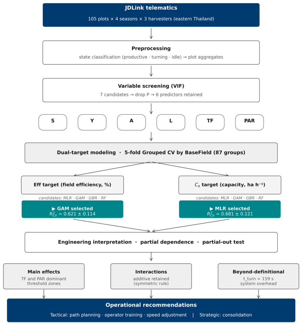
This study used operational data collected from three John Deere CH570 single-row chopper sugarcane harvesters (Deere & Company, Moline, IL, USA; model year 2020) operating in Sakaeo and Prachinburi provinces, eastern Thailand. Each harvester is powered by a PowerTech 9.0 L six-cylinder diesel engine rated at 251 kW (337 hp), with a maximum travel speed of approximately 24.6 km·h⁻¹. According to the contractor’s deployment records, each was operated by a single dedicated operator across all four seasons. Data were recorded over four consecutive harvesting seasons (2019/20, 2020/21, 2021/22, and 2022/23), covering 105 field plots under commercial harvesting conditions. Eastern and northeastern Thailand are predominantly rainfed sugarcane production regions [17]. The plots sampled here therefore represent the dominant rainfed production mode that underpins most Thai sugar mill supply. Figure 1 summarizes the overall study workflow from JDLink data acquisition through preprocessing, variable screening, dual-target modeling, engineering interpretation, and operational recommendations.

Data flow from JDLink telematics (105 plots × 4 seasons × 3 harvesters in eastern Thailand) through preprocessing and variable screening, into dual-target modeling (Eff and C_a), engineering interpretation (partial dependence and partial-out testing), and operational recommendations (tactical and strategic).

Operational data were acquired through the JDLink telematics system (Deere & Company, Moline, IL, USA), which records GPS position, ground speed, and yield sensor output at regular intervals during field operations. Plot boundaries and geometric parameters were derived from GPS trajectories using QGIS software (version 3.28; [18]). The dataset therefore reflects practical variability in field geometry, crop condition, and machine operation, rather than controlled experimental settings. Operational-state and telematics-derived data have been shown to provide a valid basis for agricultural machinery performance assessment, including field-efficiency estimation from positioning data and sugarcane harvester modeling from onboard machine measurements [9,19]. The present dataset extends the authors’ earlier GNSS-based work on sugarcane harvester performance in eastern Thailand toward a field-level telematics framework under commercial operating conditions [6,7].

Telematics records were preprocessed plot-by-plot. Operational state was inferred from the JDLink ground-speed channel together with the cutter-engagement flag: productive operation was defined as periods with cutter engaged and ground speed above 0.5 km·h⁻¹, headland turning as cutter-disengaged movement on field margins, and idle as stationary periods within the plot. A turn was counted whenever a continuous productive segment terminated and the next productive segment began on a parallel adjacent row. The yield sensor was operator-calibrated at the start of each season against truck-scale weights for at least three loads per harvester.

The modeling dataset comprised 105 plot-level observations collected across the four seasons. All predictors used in the final models (travel speed (S), crop yield (Y), plot area (A), average row length (L), turning frequency (TF), perimeter-to-area ratio (PAR)) were complete for all observations, so no rows were excluded for missing predictor values. The dataset is structured with Field ID and harvest season as separate columns. These 105 observations span 87 unique Field IDs (hereafter ‘BaseField’ groups for cross-validation grouping), since some fields were harvested across multiple seasons. Grouped cross-validation was conducted by BaseField to prevent cross-season data leakage. Each plot-level observation summarizes many thousands of raw telematics records (operational state, ground speed, position, and yield-sensor output) aggregated over one complete harvesting campaign on one plot during one season.

Telematics Preprocessing Workflow

Because the reproducibility of operational state detection is fundamental to all downstream metrics, the preprocessing steps are documented explicitly. Raw JDLink records were aggregated per plot using the following sequence: (1) spatial clipping to the surveyed plot polygon in QGIS; (2) classification into productive (cutter engaged, ground speed > 0.5 km·h⁻¹), turning (cutter disengaged but moving within an 8 m headland buffer from the plot boundary), or idle (stationary, ground speed ≤ 0.5 km·h⁻¹ for at least 5 s, regardless of cutter state); (3) counting turns as transitions from one productive segment to the next on a different row, with row assignment determined by perpendicular projection onto boundary-derived row vectors; (4) computation of T_total as state-classified time within the plot from first to last productive record; and (5) derivation of S as the mode of the productive ground-speed distribution binned in 0.1 km·h⁻¹ intervals.

The 0.1 km·h⁻¹ bin matches sensor effective resolution; sensitivity analysis (reported in Section 2.3.1) confirmed that 0.05, 0.1, or 0.2 km·h⁻¹ bins, or mean/median in place of mode, changed coefficient magnitudes by <5% without affecting sign or significance. Yield monitor output was operator-calibrated at the start of each season against truck-scale weights for at least three loads per harvester; residual within-season drift is a documented uncertainty source at throughput extremes.

Crop yield (Y) was provided by the onboard JDLink yield monitor, which integrates throughput sensor signals over the harvested area. The dataset spans the observed range 22.5–168.4 t·ha⁻¹.

Prior to model development, the dataset was screened for completeness and consistency. Exploratory analysis confirmed no critical missingness and no outliers severe enough to invalidate modeling.

Table 1. Descriptive statistics of study variables.

Variable	Unit	Mean	SD	Min	Max
Travel speed	km·h−1	4.12	0.68	2.42	5.80
Crop yield	t·ha−1	69.9	29.9	22.5	168.4
Plot area	ha	2.96	2.08	0.36	10.68
Average row length	m	236.2	104.0	108.1	629.7
Turning frequency	turns·ha−1	35.9	14.7	9.73	93.4
Perimeter-to-area ratio	m−1	0.035	0.015	0.014	0.084
Field efficiency	%	50.6	11.6	24.8	80.0
Harvesting capacity	ha·h−1	0.340	0.091	0.113	0.554

summarizes the descriptive statistics of all study variables.

2.2. Response Variable Definitions

Two response variables were analyzed separately because they represent different aspects of harvester performance. Both follow the ASAE EP496.3 machinery management standard [20]. Harvesting capacity (C_a, ha·h⁻¹) is the realized area throughput and calculated using Equation (1).

$$C_{\mathrm{a}}={\displaystyle \frac{A}{T_{\mathrm{t}\mathrm{o}\mathrm{t}\mathrm{a}\mathrm{l}}}}$$

(1)

where A is harvested plot area (ha) and T_total is total field time (h: productive + turning + idle). Theoretical field capacity (C_t, ha·h⁻¹) is the maximum possible throughput under continuous full-width operation and calculated using Equation (2).

$$C_{\mathrm{t}}={\displaystyle \frac{S \times w}{10}}$$

(2)

where S is the representative travel speed (km·h⁻¹, mode of productive ground speed) and w is row spacing (m); the factor 10 converts km·h⁻¹ × m to ha·h⁻¹. Field efficiency is calculated using Equation (3).

$$Eff={\displaystyle \frac{C_{\mathrm{a}}}{C_{\mathrm{t}}}} \times 100$$

(3)

Eff reflects how effectively available time converts to productive harvesting. Because row spacing was approximately constant, it was not included as a separate explanatory variable.

Algebraic relationships among response variables. Substituting Equation (1) and Equation (2) into Equation (3) yields Eff = (10 × C_a)/(S × w); with approximately constant w, Eff, C_a, and S are algebraically related through this identity. S also appears in the denominator of Eff via C_t. These algebraic relationships are referenced in the interpretation of individual-predictor effects.

2.3. Explanatory Variables

2.3.1. Engineering-Based Variable Selection

The explanatory variables were selected based on their physical or operational relevance to sugarcane harvester performance, organized into three engineering domains.

Machine kinematics and mass flow. Travel speed (S, km·h⁻¹) is the primary kinematic input determining feed rate into the basecutter and chopper assemblies. For each plot, S was defined as the mode of the productive-state ground-speed distribution (cutter engaged, ground speed > 0.5 km·h⁻¹) binned at 0.1 km·h⁻¹. The mode was chosen over the arithmetic mean because per-plot speed distributions are typically bimodal—a stable working-speed peak plus a low-speed tail from row-end deceleration and brief in-field stops—so the mode tracks the operator’s preferred working speed without contamination by these transients. Sensitivity comparison using mean or median in place of mode produced model rankings unchanged in direction (mean-based S reduced C_a R²_CV by ≈0.01; median-based by ≈0.005). Crop yield (Y, t·ha⁻¹), from the onboard yield monitor, represents the mass-flow constraint. Exploratory screening confirmed a strong inverse association between S and Y, consistent with operator behavior of reducing speed in heavy crops.

Spatial and geometric constraints. Plot area (A, ha) defines geometric scale. Average row length (L, m) is the most critical geometric constraint: rows shorter than a minimum threshold substantially increase turning-to-cutting time ratio. L is computed directly from plot geometry as the average pass length when all rows are conceptually unrolled into a single straight line of width w using Equation (4).

$$L_{\mathrm{a}\mathrm{v}\mathrm{g}}={\displaystyle \frac{A}{w \times n}}$$

(4)

where A is the harvested plot area (m²), w is row spacing (m), and n is the total number of rows, counted from the boundary geometry and row spacing on GIS. The numerator A/w is the ideal total productive distance—the length obtained by laying every row end-to-end as a single strip of width w—and dividing by n yields the average pass length per row. Plots with internal obstacles (ponds, trees, structures) are handled seamlessly because both A and n come directly from the GIS plot polygon, with rows defined by perpendicular projection onto boundary-derived row vectors and obstacles excluded from A. Dimensionally L = m²/(m) = m. Perimeter-to-area ratio (PAR, m⁻¹) indexes shape complexity: compact plots have low PAR; narrow or irregular plots have high PAR.

Operational discontinuity. Turning frequency (TF, turns·ha⁻¹) quantifies non-productive interruptions per unit area. Each headland turn requires deceleration, multi-point reversal, row realignment, and cutter re-engagement. TF was computed independently from telematics-derived turn counts and plot area, not derived from efficiency.

Structural relationship between TF and Eff. Although computed independently, TF and Eff are mechanistically linked through T_total: each turn adds turning time, inflating T_total, reducing C_a via Equation (1) and Eff via Equation (3). The strong inverse correlation (r = −0.806) is therefore partly the empirical magnitude of a theoretically expected relationship rather than an unexpected discovery. This analysis contributes by quantifying the magnitude and shape of this expected relationship in commercial telematics data—particularly the operating range over which incremental turns produce the largest Eff penalty—and by confirming reproducibility across multiple seasons.

This variable structure is consistent with prior evidence that field geometry strongly affects machinery efficiency, particularly through shape descriptors and turning-related time losses [13,14,15]. In sugarcane harvesting specifically, maneuvering time is a major productivity bottleneck, while machine throughput remains mechanically constrained by the interaction between forward speed and crop load [21,22].

2.3.2. Multicollinearity Screening

Following engineering-based selection, the variable set was screened for multicollinearity using the variance inflation factor (VIF) and calculated using Equation (5).

$${VIF}_j={\displaystyle \frac{1}{1 - R_j^2 }}$$

(5)

where R²_j is the coefficient of determination from regressing predictor j on all remaining predictors. Values exceeding 5 indicate substantial redundancy that may destabilize coefficient estimates. Where collinearity involved engineering-overlapping variables, the variable with stronger engineering interpretability was retained.

An initial screening of seven candidate predictors (S, Y, A, L, TF, PAR, and P) revealed that perimeter (P) exhibited a VIF of 3.76. Although this is below the conventional VIF threshold of 5, P represents definitional redundancy with A and PAR (since PAR = P/A by construction), and retaining P alongside A and PAR would introduce nonlinear multicollinearity via this product relationship. Because PAR already encodes perimeter information relative to plot area while providing more interpretable shape information, P was removed. After removal, all VIF values fell below 3.0 (

Table 2. VIF values for the final predictor set.

Variable	Domain	VIF
S	Machine kinematics	2.79
Y	Mass flow	2.90
A	Spatial scale	2.68
L	Geometric constraint	2.79
TF	Operational discontinuity	2.75
PAR	Shape complexity	2.36

). The variable selection logic can be summarized as: engineering relevance determined which variables entered the candidate set; VIF screening determined which variable left. This sequence ensures that the final set is driven by physical reasoning rather than purely statistical criteria.

2.4. Modeling Framework

The modeling framework was designed around the principle that engineering relevance and interpretability take priority over marginal gains in predictive accuracy. The model set was selected to compare interpretable linear, additive nonlinear, and tree-based nonlinear structures, consistent with recent agricultural modeling studies showing that model suitability depends on response behavior and validation context [23]. We do not present this comparison as a methodological innovation—selecting the model best suited to each target is standard practice. Rather, we use the comparison as an empirical test of whether efficiency and capacity, observed under commercial telematics conditions, exhibit different response structures that are better represented by models matched to each response’s functional shape.

2.4.1. Multiple Linear Regression

For both response variables, multiple linear regression (MLR) was used as the baseline model and calculated using Equation (6). MLR provides a transparent, familiar reference. All six predictors were retained in the MLR model based on their engineering justification rather than statistical significance; stepwise selection was not applied, consistent with the recommendation that predictor sets should be prespecified from domain knowledge to avoid inflated type-I error and unstable model structures [24].

$$y={\beta }_0 + {\mathit{\Sigma }}_{\mathrm{j}} {\beta }_{\mathrm{j}} x_{\mathrm{j}}$$

(6)

2.4.2. Spline-Based Generalized Additive Model

For field efficiency, the primary model was a generalized additive model (GAM) implemented via spline basis expansion. GAMs extend linear models by replacing each linear term with a smooth, nonlinear function of the predictor, while retaining additive structure that permits independent interpretation of each variable’s effect [25,26].

The smooth functions calculated using Equation (8) were approximated using cubic spline basis expansion (SplineTransformer; degree = 3, three knots per predictor) followed by Ridge regression, with the smoothing penalty α selected per outer fold via an inner 4-fold grouped cross-validation over (0.01, 0.1, 1.0, 10.0) (nested cross-validation). Three knots per predictor is a conservative setting for n = 105. Knot sensitivity was tested explicitly by re-fitting the GAM with three, five, and seven knots per predictor. This formulation is functionally equivalent to a canonical penalized additive model implemented via the scikit-learn pipeline.

Eff = β₀ + Σ_j f_j(x_j) + ε

(7)

where f_j(x_j) is the smooth function for predictor j, approximated through the B-spline basis expansion:

f_j(x_j) = Σ_k β_jkB_jk(x_j)

(8)

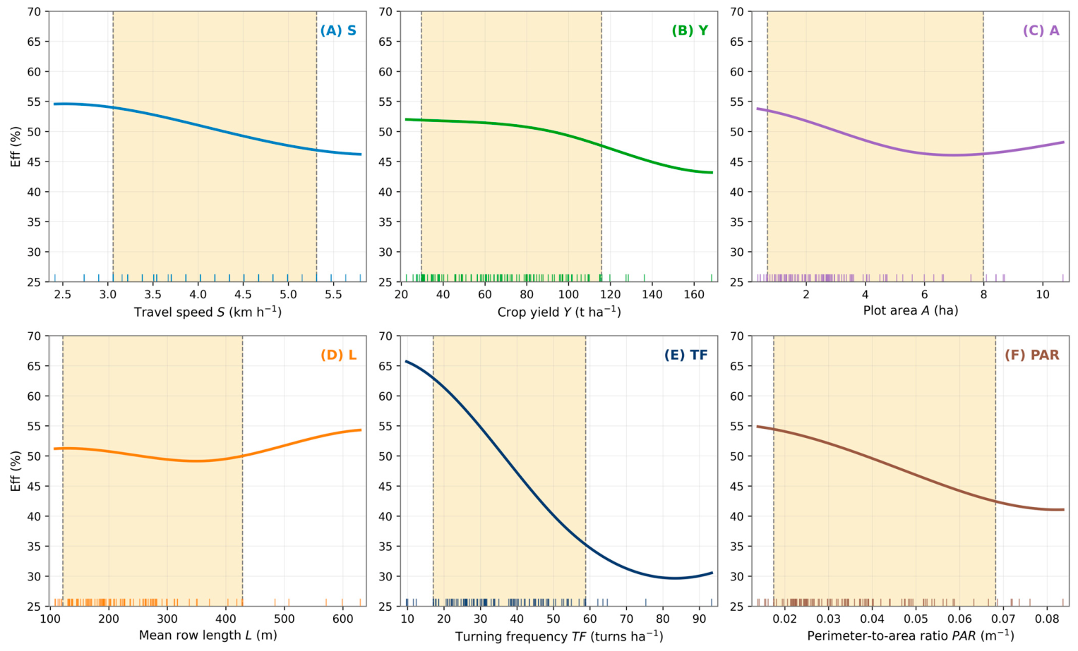
where B_jk(x_j) are the cubic B-spline basis functions generated by SplineTransformer (degree = 3, three uniformly spaced knots spanning the observed range of predictor j, producing 4 basis functions per predictor). The full feature space thus comprises 6 × 4 = 24 spline terms plus an intercept (25 parameters total). The Ridge penalty applied to (β_jk) acts as the smoothing mechanism—larger α shrinks coefficients toward zero, reducing the effective degrees of freedom of the fitted model (≈13.2 at the nested-CV-selected α = 0.1). The fitted f_j functions are visualized as partial dependence curves in Figure 2.

2.4.3. Boosting and Random Forest

For capacity (C_a), nonlinear tree-based candidates were evaluated because structured operational data in agriculture often benefit from flexible ensemble learners that can represent nonlinear responses and interaction structure without requiring explicit specification [9,27].

Gradient Boosting Regression (GBR) constructs an ensemble of shallow decision trees sequentially, where each successive tree is trained on the residuals of the preceding ensemble [28]. The tuning grid was designed to span from the parsimony-favoring corner (additive stumps with max-depth = 1, analogous to the GAM structure) to moderately richer candidates (max_depth = 2 or 3), allowing the inner cross-validation to choose deeper alternatives if the data support them [28].

Random Forest Regression (RF) constructs an ensemble of independent decision trees, each trained on a bootstrap sample of the data with a random subset of features selected at each split. RF was included because its variance-reduction mechanism (averaging across decorrelated trees) differs from GBR’s bias-reduction approach, providing complementary evaluation of nonlinear model suitability.

The full factorial design (all four models × both targets) was evaluated to provide complete cross-target model comparison. Hyperparameters were chosen to balance expressiveness against overfitting on the 105-observation dataset: Hyperparameters for GBR and RF were selected via nested 4-fold grouped cross-validation (the same inner-CV protocol applied to GAM α). GBR was tuned over max-depth ∈ (1, 2, 3), learning_rate ∈ (0.05, 0.1), and n_estimators ∈ (50, 100, 200) (18 combinations); RF was tuned over max_depth ∈ (3, 5, 7, None) and n_estimators ∈ (100, 200) (8 combinations). The grids deliberately span the parsimony-favoring corner where additive-stump GBR and shallow RF lie, while also allowing the inner CV to choose deeper alternatives if the data support them.

2.4.4. Implementation

All models were implemented in Python (version 3.10) using scikit-learn (version 1.3; [29]). The GAM was implemented as SplineTransformer (degree = 3, n-knots = 3) followed by Ridge regression with α selected per outer fold by an inner 4-fold grouped cross-validation over (0.01, 0.1, 1.0, 10.0) (nested cross-validation). R²_CV and train-validation gap values reported for the GAM are outer-fold estimates that do not condition on the test data. Standardized regression coefficients are reported as fully standardized effects, b × SD(x)/SD(y), so that they are dimensionless and directly comparable across predictors with different units.

2.5. Model Validation Strategy

Model performance was evaluated using 5-fold grouped cross-validation. Observations were grouped by BaseField to prevent data from the same underlying field appearing in both training and validation partitions across seasons within a single fold.

BaseField groups correspond directly to the Field ID column in the dataset, so that, for example, field ‘119287’ harvested in both 2020/21 and 2021/22 shares the same BaseField group, ensuring both observations appear in the same fold. Of the 87 BaseField groups, 72 contain one observation (single-season fields), 12 contain two observations, and three contain three observations from different harvesting seasons. Observations were sorted by BaseField prior to fold assignment to ensure deterministic reproducibility.

This grouping was necessary because observations from the same BaseField across different seasons share soil conditions, crop management history, and operator behavior that would artificially inflate validation performance under random splitting. By holding out entire BaseField groups, the validation provides a more realistic estimate of how each model would perform on genuinely unseen field conditions—the scenario that matters for operational deployment [23,30].

2.6. Evaluation Metrics and Statistical Comparison

Two complementary metrics were used. Root mean square error (RMSE) quantifies prediction error in the original units of the response variable. Coefficient of determination (R²) quantifies the proportion of response variance explained, enabling comparison across targets with different scales. Both were calculated within the grouped cross-validation framework, so reported values reflect generalization to unseen BaseField groups rather than resubstitution accuracy. To characterize the stability of these estimates, mean and standard deviation across the five folds are both reported. The train–validation R² gap (mean training R² minus mean validation R²) is reported as a complementary indicator of overfitting risk.

Pairwise model comparisons were tested with the Wilcoxon signed-rank test on fold-level R² values (two-sided, exact distribution) for the principal contrasts of interest: GAM versus MLR for each target, and MLR versus GBR/RF for C_a. With only five folds, the Wilcoxon exact two-sided p-value cannot fall below approximately 0.0625 even when all fold differences agree in sign, so absence of nominal significance under this test should be interpreted in light of its very limited statistical power rather than as evidence of equivalence. The train–validation gap and consistency of fold-level direction therefore serve as complementary, not redundant, evidence. Accordingly, these p-values are reported for transparency only and were not used as a selection criterion; model choice rested on effect size, train–validation gap, fold-level consistency, response behavior, and parsimony.

Partial-out test: separating definitional from operational TF effect. TF and Eff are mechanically linked through the time-budget identity: each additional turn consumes working time and therefore reduces Eff by a predictable amount even in the absence of any operational variation. A natural question is how much of the observed TF–Eff correlation reflects this definitional coupling alone versus additional operational overhead (queueing for wagons, engagement losses, operator reset time) that is not captured by a pure kinematic model. To separate the two, a single-parameter structural model with a lumped per-turn time t_turn was fitted: Eff_nom = 100/(1 + C_t × TF × t_turn), where t_turn is a single lumped non-productive-time parameter per turn, fitted by least squares across all plots. The residual (Eff − Eff_nom) was then regressed on TF both linearly and via a 3-knot spline. A residual slope indistinguishable from zero would indicate that TF’s univariate effect on Eff is essentially mediated by the time-budget identity; a substantial remaining structure would indicate operationally independent content.

2.7. Interpretation Framework

Model interpretation followed a predefined three-step framework intended to move beyond model comparison toward defensible explanation of the physical and operational mechanisms underlying harvester performance.

Step 1—Main effects. The first step identifies the direction, magnitude, and shape of each explanatory variable’s individual effect on the response. For efficiency, these effects are examined through the smooth additive functions estimated by the GAM, visualized as partial dependence plots. For capacity, MLR regression coefficients (with fully standardized β for cross-predictor magnitude comparison) provide the equivalent representation.

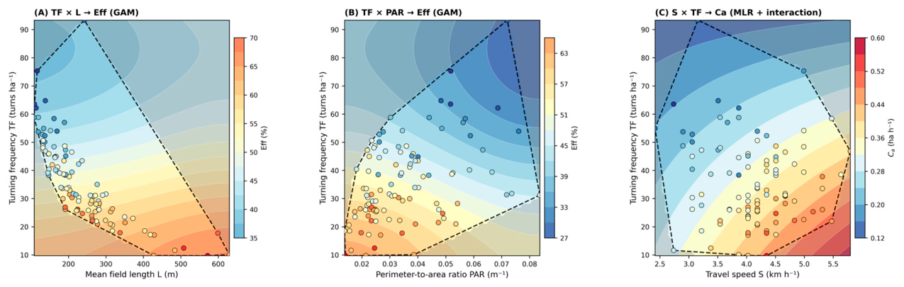
Step 2—Interaction effects. The second step examines operationally meaningful combinations between predictors. Three pairs were pre-specified based on engineering reasoning: TF × L (whether short rows amplify the per-turn penalty), TF × PAR (whether shape complexity modulates turning cost), and S × TF (whether speed adjustment can offset turning losses). The S × Y and A × PAR pairs considered earlier in our planning were assessed informally during exploratory analysis but did not survive the pre-specification step because their main effects were already captured by stronger correlated predictors. The purpose is not to enumerate all statistical interactions but to test the combinations most relevant to harvester behavior.

Step 3—Operational implications. The third step translates statistical patterns into field-level recommendations. This includes identifying approximate threshold zones (rather than precise threshold values, given uncertainty in the smooth fits) and scenario comparisons.

This interpretation strategy is aligned with current agricultural XAI practice, where feature-level explanation is used to convert predictive models into operational insight [11,13], and is consistent with recent agricultural machinery studies showing that transparent interpretation frameworks can preserve engineering usefulness even when flexible machine-learning models are employed [31].

3. Results

3.1. Overall Model Performance and Statistical Comparison

Predictive performance was evaluated using 5-fold GroupKFold grouped by BaseField (87 groups, 105 observations). All four candidate models (MLR, GAM, GBR, RF) were evaluated against both targets; results are summarized in

Table 3. Cross-validated predictive performance.

Target	Model	R2CV (Mean ± SD)	CV-RMSE (Mean ± SD)	Train–Val R2 Gap
Field Efficiency, Eff (%)	GAM ★	0.621 ± 0.114	6.60 ± 1.14%-pts	0.118
	MLR	0.601 ± 0.113	6.76 ± 1.00%-pts	0.111
	RF	0.557 ± 0.154	7.08 ± 1.07%-pts	0.358
	GBR	0.544 ± 0.161	7.24 ± 1.46%-pts	0.302
Harvesting Capacity, Ca (ha·h−1)	GAM	0.682 ± 0.124	0.047 ± 0.008	0.112
	MLR ★	0.681 ± 0.121	0.047 ± 0.006	0.096
	GBR	0.656 ± 0.140	0.049 ± 0.009	0.210
	RF	0.621 ± 0.105	0.052 ± 0.008	0.322

★ = primary model selected. Wilcoxon two-sided exact p-values for paired fold R².

with fold-level standard deviations. R²_CV and train-validation gap values reported for GBR and RF are outer-fold estimates that do not condition on the test data.

For field efficiency (Eff), the GAM achieved mean R²_CV = 0.621 ± 0.114 under nested cross-validation with MLR essentially tied (0.601 ± 0.113). Among tuned tree-based candidates, GBR achieved 0.544 ± 0.161 and RF 0.557 ± 0.154. The GAM–MLR gap of 0.020 is not statistically significant under the Wilcoxon signed-rank test on paired fold R² values (p = 0.31, two-sided, n = 5 folds); the 95% bootstrap confidence interval on the paired difference ([−0.005, +0.045]) straddles zero. The GAM train–validation R² gap (0.118) was substantially smaller than that of GBR (0.302) and RF (0.358), confirming that tree-based flexibility produced overfitting rather than improved generalization. Selection of GAM as the primary Eff model is therefore based on its ability to represent the threshold-shaped TF response, which the linear MLR cannot express in its functional form, rather than on a R²_CV advantage; this choice is discussed further in Section 4.2.

For harvesting capacity (C_a), MLR achieved mean R²_CV = 0.681 ± 0.121 and GAM (under nested cross-validation) achieved 0.682 ± 0.124, with GBR 0.656 ± 0.140 and RF 0.621 ± 0.105 among tuned tree-based candidates. The GAM–MLR gap of 0.002 is not statistically significant under the Wilcoxon signed-rank test (p = 0.81, two-sided, n = 5 folds), and the paired Cohen’s d (0.03) is in the negligible range; the 95% bootstrap confidence interval on the paired difference ([−0.039, +0.050]) straddles zero. MLR train–validation gap (0.096) and GAM gap (0.112) were both substantially smaller than tree-based candidates (GBR 0.210, RF 0.322), again indicating that tree flexibility did not generalize. Under the principle of parsimony, MLR is retained as the primary C_a model; the GAM partial smooths for the dominant C_a predictors (S, TF, PAR) are themselves approximately linear across the observed range, supporting a near-linear capacity structure as a substantive engineering finding rather than a modeling limitation.

3.2. Main Effects on Field Efficiency

The GAM R²_CV of 0.621 for Eff corresponds to fold-mean RMSE = 6.60 ± 1.14%-points (Table 3; ≈57% of SD(Eff) = 11.57), a moderate rather than tight fit: ≈38% of Eff variance and ≈32% of C_a variance remain unexplained. The partial-effect interpretation that follows therefore concerns the structured portion of the response, not the full physical system.

The GAM partial dependence plots for Eff reveal nonlinear effects across the six predictors (Figure 2). Pearson correlations reported below are from exploratory analysis of the full dataset and are provided for descriptive context only. Predictor importance can be quantified in three complementary ways: univariate Pearson correlation (marginal association), MLR standardized coefficient β_std (per-SD conditional effect), and GAM partial-effect range (total conditional effect over the observed range).

Table 4. Predictor importance for field efficiency under three complementary metrics (n = 105).

Variable	Pearson r	GAM PDP Range (%-pts)	Rank (PDP)
TF	−0.806	28.96	1
PAR	−0.492	12.33	2
S	−0.019	8.36	3
A	+0.449	7.44	4
Y	−0.108	4.44	5
L	+0.616	2.12	6

provides the full comparison; the three metrics rank variables differently because they answer different questions. Turning frequency (TF) dominates across all three metrics; perimeter-to-area ratio (PAR) consistently ranks second in the conditional metrics (β_std, PDP range), while mean row length (L) has the strongest univariate correlation but a comparatively small conditional effect after controlling for TF and PAR.

Pearson r = univariate correlation with Eff. MLR β_std values and significance levels are reported in

Table 5. MLR regression coefficients for field efficiency (Eff).

Variable	b	SE	p	βstd	Sig
TF	−0.541	0.0729	<0.001	−0.689	***
PAR	−222.97	62.97	<0.001	−0.298	***
S	−3.751	1.415	0.009	−0.222	**
A	−1.056	0.499	0.037	−0.189	*
Y	−0.0642	0.0336	0.059	−0.166	ns
L	+0.0124	0.0100	0.220	+0.111	ns
—	98.01	9.352	<0.001	—	***

*** p < 0.001, ** p < 0.01, * p < 0.05.

(MLR Eff coefficients). GAM PDP range = max–min of the partial dependence over the 5th-to-95th percentile of each predictor, computed with scikit-learn partial_dependence (kind = ‘average’, grid_resolution = 50) from the GAM fitted with α = 0.1, the most frequent selection from the nested-CV grid (0.01, 0.1, 1.0, 10.0). The three metrics rank variables differently because they answer different questions: Pearson r captures marginal association (including indirect effects through correlated predictors); MLR β_std reports per-SD conditional effect; and GAM PDP range reports the total conditional effect across the predictor range.

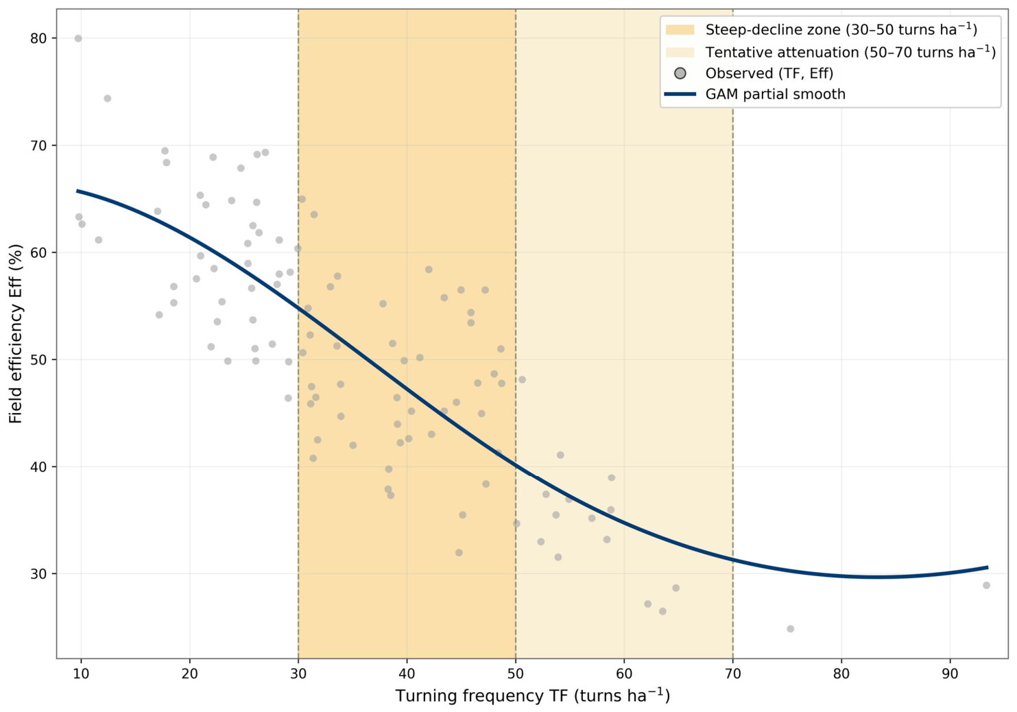
Turning frequency (TF) was the dominant predictor of field efficiency (Pearson r = −0.806). The partial dependence curve for TF shows a nonlinear response (Figure 3): Eff declines continuously as TF increases, with the largest marginal penalty—i.e., each additional turn per hectare reduces Eff most strongly—occurring between approximately 30 and 50 turns·ha⁻¹. Beyond approximately 70 turns·ha⁻¹ the curve flattens: additional turns impose progressively smaller incremental Eff losses, likely because fields with very high TF already operate in a turn-dominated regime where remaining time is consumed by other overhead. We label these as approximate operational zones rather than precise thresholds because the spline estimate is sensitive to knot placement and dataset coverage at the upper end of the range. Strong relationship reflects the structural coupling between TF and Eff through total field time; the GAM’s contribution is to quantify the magnitude and shape of that relationship in commercial telematics data and to identify the operating range over which the per-turn penalty is most pronounced. Much of this steep-then-flat shape comes from the time-budget identity itself, which curves the same way. After that identity is removed, only a small but significant nonlinear component remains (residual spline F(3, 100) = 6.74, p < 0.001; Section 3.2), so the threshold mainly reflects the identity’s shape rather than a separate operational effect.

Operational component of TF effect. Applying the constant-turn-time partial-out procedure, the fitted lumped per-turn non-productive time was t_turn = 159 s (95% CI: 149–170 s, cluster bootstrap by BaseField). This value is not a pure mechanical turning duration—typical chopper-harvester turns under dedicated-headland operation are 30–60 s [21,32,33]—but a single lumped equivalent that absorbs all TF-correlated non-productive time per turn observed in telematics. Components attributable per turn therefore include the physical maneuver, in-field repositioning and cutter re-engagement, and the coordination with the infield loading vehicle that is structurally tied to each headland event. The fitted value is system-level overhead per TF event in commercial Thai operation. The definitional model Eff_nom = 100/(1 + C_t × TF × t_turn) explained 56.0% of Eff variance in-sample and 47.6% under grouped CV—close to the 60.1% achieved by full MLR. The residual Pearson correlation with TF fell to r = −0.005, and the linear residual slope was indistinguishable from zero (t(103) = −0.05, p = 0.96). A three-knot spline nevertheless added significant nonlinear structure beyond the linear term (nested spline-versus-linear F(3, 100) = 6.74, p < 0.001; ΔR² = 16.8 percentage points by unpenalized least squares), and the corresponding penalized (ridge) GAM fit gave a residual R² of 14.5% (the lower value reflecting ridge shrinkage). The incremental R²_CV of full MLR over the definitional model was +0.125. The univariate TF–Eff association is therefore substantially captured by a single-parameter time-budget model, with a modest beyond-definitional component that retains nonlinear structure—consistent with the GAM partial smooth interpretation in Figure 3 and supporting the additive-nonlinear modeling choice for Eff. By contrast, residual correlations remained substantial for Y (r = −0.37) and S (r = +0.41), consistent with beyond-definitional operational content for those predictors. Stratified fits across plot-size tertiles confirm the lumped value is independent of plot size (Spearman r between per-plot implied turn time and A: +0.02, p = 0.86; with L: +0.06, p = 0.52), supporting interpretation as a structural property of the field-system configuration rather than a per-plot artifact. The engineering interpretation of the elevated lumped value under Thai smallholder field conditions is taken up in Section 4.4.

Knot sensitivity. To assess whether the threshold zone is an artifact of the spline configuration, the GAM was re-fitted with three, five, and seven knots per predictor. Mean R²_CV for Eff was 0.621 ± 0.114 (3 knots), 0.554 ± 0.134 (5 knots), and 0.533 ± 0.100 (7 knots) under nested cross-validation, with train–validation gaps of 0.118, 0.182, and 0.255, respectively. Increasing knot density therefore reduces both predictive accuracy and parsimony. The qualitative shape of the TF curve—monotonic decline with attenuated slope at the high end—was preserved across knot counts; the location of the steepest-decline zone shifted by less than 5 turns·ha⁻¹. The three-knot configuration was retained because it minimized the train–validation gap and is the most defensible setting at n = 105.

Perimeter-to-area ratio (PAR) (Pearson r = −0.492) reflects shape complexity. The partial effect of PAR is negative and approximately monotonic across the observed range, indicating a consistent shape penalty without the threshold nonlinearity seen for TF.

Field area (A) shows a moderate positive association (Pearson r = +0.449), partially mediated through its geometric relationship with TF and L. After conditioning on TF, L, and PAR, the residual partial effect of A is attenuated.

Travel speed (S) and crop yield (Y) exhibit weak univariate associations with Eff (Pearson r = −0.019 and −0.108, respectively). The GAM partial smooth for S is broadly flat within the observed range (2.4–5.8 km·h⁻¹), although the MLR linear coefficient on S remains nominally significant (Table 5, b = −3.751, p = 0.009, β_std = −0.222); Y shows negligible partial effect at the field-mean scale in both specifications. The small partial smooth for S on Eff in the GAM is consistent with the algebraic coupling between S and Eff via C_t.

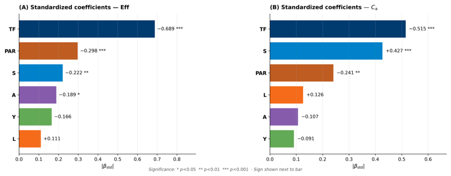
For comparison, the MLR benchmark coefficients for Eff are reported in Table 5. The same dominance of TF and PAR is confirmed, with TF exhibiting the largest fully standardized effect (β_std = −0.689). The MLR structure captures 60.1% of Eff variance under cross-validation (Table 3), comparable to 62.1% for the GAM (under nested cross-validation)—the marginal R²_CV difference understates the GAM’s value, which lies in capturing the threshold-shaped TF response that MLR cannot represent (Figure 3).

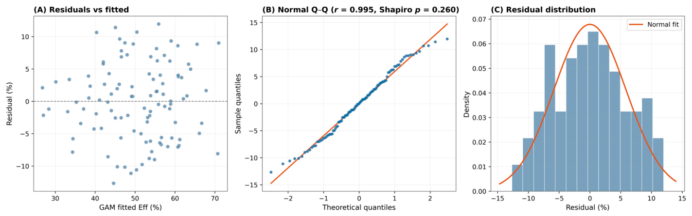
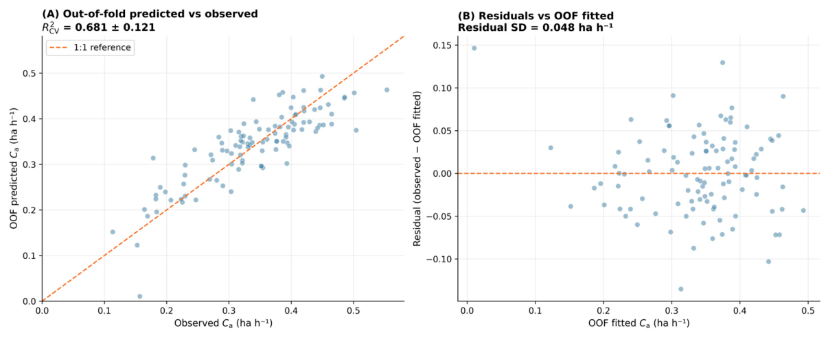
GAM diagnostics (Figure 4) confirm the validity of the additive specification: residuals are centered with SD = 5.88%-pts, normality is not rejected (Shapiro–Wilk p = 0.260; Q–Q correlation = 0.995), and the effective degrees of freedom ≈ 13.2 (well below the nominal 25 basis dimensions) confirm that Ridge regularization is active.

3.3. Main Effects on Harvesting Capacity

The MLR model for C_a (R²_CV = 0.681 ± 0.121) provided a stable linear description of capacity variation. Regression coefficients are reported in

Table 6. Full-data MLR regression coefficients for harvesting capacity (C_a).

Variable	b	SE	p	βstd	Sig
TF	−3.17 × 10−3	5.02 × 10−4	<0.001	−0.515	***
S	+0.0566	0.0097	<0.001	+0.427	***
PAR	−1.414	0.4337	0.0015	−0.241	**
A	−4.67 × 10−3	3.44 × 10−3	0.177	−0.107	ns
Y	−2.77 × 10−4	2.32 × 10−4	0.234	−0.091	ns
L	+1.10 × 10−4	6.91 × 10−5	0.115	+0.126	ns
—	0.278	0.0644	<0.001	—	***

*** p < 0.001, ** p < 0.01.

, and model diagnostics in Figure 5.

Turning frequency (TF) was the dominant predictor of C_a (Pearson r = −0.729; b = −3.17 × 10⁻³ ha·h⁻¹ per turn ha⁻¹; β_std = −0.515), still the largest standardized effect among all predictors. The convergence of TF as the primary driver of both Eff and C_a reflects the central role of field geometry in constraining harvester performance.

Travel speed (S) is the only predictor with a positive coefficient (b = +0.0566 ha·h⁻¹ per km·h⁻¹; β_std = +0.427), consistent with the direct relationship between speed and area coverage rate. The positive effect of S on C_a contrasts with its near-zero marginal association with Eff in the GAM partial smooth (the MLR linear coefficient on S in the Eff model remains nominally significant, as noted in Table 5), supporting the distinction between throughput rate and time efficiency.

Perimeter-to-area ratio (PAR) has a strongly negative coefficient (b = −1.414; β_std = −0.241). PAR ranks among the top predictors in both models, reinforcing that field shape irregularity penalizes performance across both dimensions.

The partial coefficients for L, A, and Y are small and statistically non-significant (p > 0.05; Table 6). These variables were retained in the model based on engineering relevance rather than statistical significance—their non-significance after joint adjustment reflects shared geometric information already captured by TF and PAR. Sign reversals for L and A likely arise from the same geometric redundancy; VIF values remain low (2.36–2.90), confirming this is residual overlap rather than severe collinearity.

3.4. Additive Structure and Interaction Assessment

An additive model structure implies that each predictor’s effect on the response combines by simple summation—the effect of TF on efficiency does not depend on the value of L, and vice versa. If interactions were present, the combined effect of two predictors would differ from the sum of their individual effects, requiring explicit interaction terms or multiplicative model structures.

Two-way interaction surfaces were examined for the three pairs pre-specified: TF × L, TF × PAR, and S × TF. For the Eff GAM, no meaningful deviation from additivity was detected. The TF × L surface (Figure 6A) shows approximately parallel contours across the observed data range, consistent with superimposed main effects; the TF × PAR surface (Figure 6B) shows a similar additive pattern; and the S × TF surface for C_a (Figure 6C) likewise shows no clear evidence of multiplicative interaction at the surface level. A formal pre-specified interaction test was then applied symmetrically to both targets using a common decision rule (improvement on 5-fold R²_CV and non-degradation of train–validation gap). TF × L and TF × PAR failed the criteria on both targets. S × TF met the criteria for C_a (ΔR²_CV = +0.018; Δgap = −0.007) but failed them for Eff (ΔR²_CV = −0.025; Δgap = +0.027). Adopting S × TF only for C_a would constitute asymmetric model selection; the additive baseline was therefore retained for both targets. This decision is also consistent with the approximately linear GAM partial smooths for C_a across the observed range of S, TF, and PAR (Section 3.3), which do not indicate a pronounced non-additive regime in the Thai commercial telematics envelope.

The confirmed additive structure implies that field geometry and operational speed affect harvester performance through largely independent pathways. Field length and turning frequency contribute through their respective mechanisms—productive-run duration and turning overhead—with no clear evidence of additional interaction beyond the main effects within the observed range. This supports the use of parsimonious additive models for operational planning under conditions comparable to those studied.

3.5. Variable Importance Summary

Figure 7 shows the absolute fully standardized coefficient (|β_std|) from the MLR full-data fits for both Eff (Figure 7A) and C_a (Figure 7B), providing a common-scale comparison of predictor influence across the two targets. Because GAM was selected for Eff on functional-form grounds rather than predictive superiority over MLR, presenting both targets through their directly comparable linear specification offers the clearest cross-target read. TF and PAR rank consistently high across both targets, confirming that field geometry is the primary structural driver of sugarcane harvester performance at the plot level.

4. Discussion

4.1. Model Suitability

The results support analyzing efficiency and capacity under model structures matching each response’s behavioral characteristics rather than forcing a single algorithm onto both. We frame this as an empirical observation rather than a methodological framework: matching model complexity to data structure is routine applied-statistics practice, and our contribution is to confirm that the expected divergence between Eff and C_a holds under commercial telematics conditions.

For Eff, GAM (under nested cross-validation) achieved mean R²_CV = 0.621 ± 0.114, with MLR essentially tied (0.601 ± 0.113), followed by tuned RF (0.557 ± 0.154) and tuned GBR (0.544 ± 0.161). Mean differences between the two additive candidates were not statistically significant under five-fold Wilcoxon testing (p = 0.31, GAM vs. MLR), but the additive train–validation gaps (0.111–0.118) were substantially smaller than those of the tuned tree candidates (GBR 0.302, RF 0.358), indicating that tree-based flexibility produced overfitting rather than better generalization [23]. Although MLR is the more parsimonious model and is statistically tied with GAM on predictive accuracy, GAM is retained as the primary Eff model because it captures the threshold-shaped TF response that MLR cannot represent; MLR remains an equally predictive linear benchmark.

For C_a, MLR achieved mean R²_CV = 0.681 ± 0.121 with the smallest train–validation gap (0.096), essentially tied with GAM under nested cross-validation (0.682 ± 0.124, gap 0.112) and well ahead of tuned tree candidates (GBR 0.656 ± 0.140, gap 0.210; RF 0.621 ± 0.105, gap 0.322). The GAM–MLR difference (0.002) was not statistically significant (Wilcoxon p = 0.81; Cohen’s d = 0.03); MLR is retained as the primary C_a model on parsimony grounds within the observed operating range. C_a’s near-linear structure under commercial telematics is a substantive outcome, not a limitation. Because GAM and MLR are statistically indistinguishable on both targets, the assignment of a “primary” model to each target is a matter of parsimony and response behavior rather than statistical superiority. Both models were fitted and evaluated on both targets throughout;

Table 7. Final model assignments for field efficiency and harvesting capacity, with structural basis. Wilcoxon p-values are reported for transparency and were not used as a selection criterion.

Target	GAM R2CV	MLR R2CV	Wilcoxon p	Selected	Basis for Selection
Eff (%)	0.621 ± 0.114	0.601 ± 0.113	0.31	GAM	Threshold-like response to turning frequency
Ca (ha·h−1)	0.682 ± 0.124	0.681 ± 0.121	0.81	MLR	Parsimony; performance tied with GAM

reports both R²_CV values side by side. Convergent rankings of the dominant predictors (TF and PAR) between an explicitly nonlinear additive model (GAM) and a linear model (MLR) provide independent confirmation that the findings are robust to functional-form choice rather than artifacts of a single modeling paradigm. Table 7 summarizes model assignments. Selections were guided by mean rank, fold-level direction, train–validation gap, and parsimony rather than statistical significance alone.

4.2. Field Geometry as the Primary Performance Driver

The dominance of turning frequency and shape-related variables across both targets reinforces the conclusion that field geometry is the primary structural constraint on plot-level harvester performance. This is consistent with prior work showing that boundary descriptors and geometric indices strongly influence machinery efficiency through effects on pass continuity, overlap, and turning demand [13,14,15].

The strong empirical role of TF must be interpreted alongside the structural coupling: each turn mechanically inflates total field time, reducing both C_a and Eff by definition. The partial-out analysis confirmed that TF’s univariate effect on Eff is largely mediated by this time-budget identity; the value added by the GAM is to quantify the operating range over which each additional turn produces the largest penalty—information the algebraic relationship alone does not provide.

PAR’s dominance as a shape descriptor has been reported previously for perennial grass harvesting [14] and in simulation-based efficiency modeling [13]. The present study extends these findings to real commercial sugarcane operations: across 105 plots and four seasons, PAR ranked among the top three predictors for both targets (Figure 7). Turning frequency’s role has also been demonstrated at the operational level in sugarcane [21]. The convergence of TF and PAR across Eff and C_a indicates that field geometry sets the performance envelope that constrains both efficiency and throughput, while operational variables—particularly travel speed—regulate performance within that envelope.

4.3. Why Harvesting Capacity Follows a Linear Structure

The linear structure of C_a under MLR warrants explicit discussion, because it contrasts with the nonlinear Eff response and may appear counterintuitive given the use of tree-based ensemble candidates.

Harvesting capacity (ha·h⁻¹) is a throughput rate that depends primarily on travel speed and the effective working time available within a field. Theoretically, effective field capacity is the product of working width, travel speed, and field efficiency (C_a = C_t × Eff = S × w × Eff/10; Equations (1)–(3); [20]). In the present dataset, row spacing (w) was approximately constant, so C_a variation was driven primarily by S and Eff—both of which exhibit linear or near-linear partial effects within the MLR structure. This is consistent with the theoretical formulation and explains why MLR captures C_a adequately. Eff and C_a are themselves coupled through this same identity; modeling them with different families therefore captures different aspects of the same underlying response surface, with each model emphasizing a different part of the operating dynamics.

Geometric factors (TF, PAR, A, L) constrain the operating time available by displacing productive harvesting with non-productive maneuvering, but this displacement occurs in proportion to the geometric structure rather than nonlinearly. The result is a linear capacity–geometry relationship well-represented by the additive structure of MLR.

This is not a failure of ML models to detect nonlinearity—GBR and RF were both applied and neither outperformed MLR under grouped cross-validation. It indicates that under the present grouped-CV design and sample size, the additional flexibility of GBR and RF did not translate into improved generalization for harvesting capacity, consistent with observations that linear baselines can match or outperform ensemble methods on structured operational data when sample sizes are moderate [27]. The contrast between Eff (nonlinear, threshold-driven) and C_a (linear, rate-driven) therefore reflects a genuine structural difference between the two performance dimensions within the observed operating range—although the two dimensions are themselves not independent quantities.

4.4. Interpreting the Lumped Per-Turn Overhead

The partial-out analysis returned a lumped per-turn time t_turn = 159 s (95% CI: 149–170 s), substantially larger than the 30–60 s mechanical turning durations reported for chopper harvesters with dedicated headland space [21,33]. The apparent discrepancy warrants engineering interpretation.

The estimate is consistent with convergent evidence: Brazilian commercial operations place harvester maneuver time at 1.50–2.00 min even with dedicated headlands and active route optimization [21], and prior stopwatch fieldwork by the present research group in eastern Thailand measured 2.00–3.00 min per turn in commercial plots. The 95% CI (2.49–2.83 min) falls fully within the stopwatch range, providing contextual corroboration across two independent estimation approaches. Stratified fits confirmed no systematic dependence on plot size.

The gap between the Thai lumped value and the Brazilian benchmark reflects a structural difference in field configuration. Brazilian commercial fields systematically allocate headland area, enabling planned three-stage maneuvers completable in tens of seconds [33], and the “P” pattern documented by Corrêa et al. [21] further shortens the tandem harvester–wagon cycle. Thai smallholder fields, by contrast, rarely allocate headland area—planting area is preserved as revenue-bearing—forcing a constrained switch-back maneuver with multiple forward–reverse cycles, wait events at harvester–wagon coordination points at both turn entry and exit [21], and diagonal re-entry into the adjacent row. The lumped estimate absorbs all repeatable plot-independent overhead that scales with the number of turns, including approach/departure slowdowns and tandem-vehicle coordination time. In this sequence, per-turn times of 120–180 s are geometrically and operationally plausible; 159 s falls comfortably within it.

Reading t_turn = 159 s as an effective operational penalty has two implications. First, the non-mechanical component provides a physical mechanism for the 30–50 turns ha⁻¹ steep-decline zone in Eff: each additional turn displaces productive time more heavily than under Brazilian or Australian benchmarks. Second, because these plots have not been reorganized to add headland space, the estimate is stable across the observed TF range.

4.5. Operational Implications for Field Planning

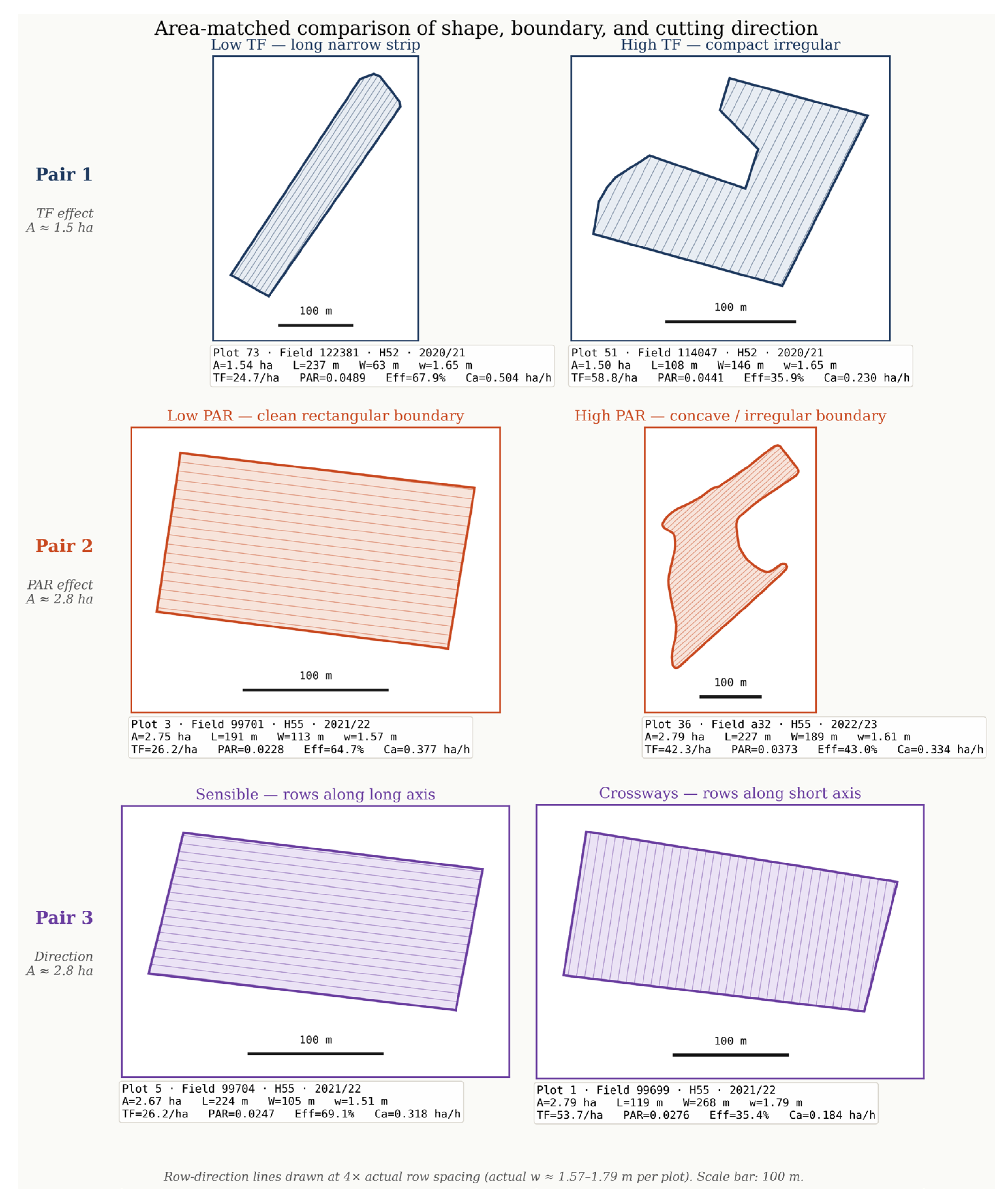
To ground the quantitative main-effect estimates, Figure 8 presents six plots from the study dataset, grouped into three area-matched comparison pairs. Holding plot area approximately constant isolates the geometric or operational factor under comparison—turning frequency (TF) driven by shape, perimeter-to-area ratio (PAR) driven by boundary regularity, and effective row length driven by harvesting direction—from the confounding effect of field size. The three pairs motivate the three operational levers discussed in the remainder of this section.

The three-step engineering interpretation framework identified several actionable patterns for harvest planners in Thai sugarcane production. Because plot-level field layout in Thailand is largely determined by smallholder land tenure, contract farming arrangements with sugar mills, and historical parcel boundaries, we separate recommendations into tactical interventions that are immediately feasible at the operator and harvest-coordinator level, and strategic interventions that depend on longer-term land or contract arrangements.

4.5.1. Tactical Interventions (Immediate, Operator-Controllable)

Harvest path planning. For a fixed boundary, TF depends on the chosen path. Where a plot can be entered from multiple sides, planning so longest passes align with the dominant axis reduces TF without changing the field—a principle illustrated by comparing the low-TF and high-TF plots of Figure 8 Pair 1, which have near-identical area but differ by a factor of 2.4 in TF. This is the highest-leverage tactical intervention because TF dominates both targets and path selection is directly under operator control.

Machine–field allocation. Sequencing high-TF plots earlier (operators fresh) and matching plots to operator skill captures gains without infrastructure change. Allocating experienced operators to high-PAR plots (Figure 8 Pair 2)—where the concave boundary forces frequent cutter disengagements at shape-induced interruptions—is a low-cost intervention.

4.5.2. Strategic Interventions (Longer-Term, Requiring Contract or Tenure Change)

Plot consolidation and layout redesign. The convergent TF and PAR dominance across both targets implies that consolidating fragmented plots and extending effective row length would yield the largest per-hectare gains. Figure 8 Pairs 1 and 3 together illustrate this at the plot level: extending effective row length—whether by reshaping an irregular plot into a longer strip (Pair 1) or by choosing the long-axis cutting direction on an existing rectangle (Pair 3)—produces efficiency gains of 30+ percentage points at equivalent plot area. The univariate correlation of L with Eff is strong (r = +0.616), but its conditional contribution after controlling for TF and PAR is small (Table 4, PDP rank 6), consistent with L operating largely through its effect on TF. Plot consolidation would therefore reduce TF and improve Eff indirectly, rather than through a row-length threshold. In the Thai smallholder sector, however, plot boundaries are typically fixed by land ownership, inherited parcel layout, and contract farming with the mill; consolidation requires land reorganization, multi-grower harvest cooperatives, or contract-level coordination. Consolidation is therefore a strategic priority for mill-level planning rather than a short-term intervention.

Obstacle removal in high-PAR plots. Internal obstacles (ponds, trees, structures) and irregular boundaries (Figure 8 Pair 2, right panel) inflate PAR and reduce mean row length. Where removable and the grower agrees, relocation or boundary straightening produces a one-time PAR reduction—feasible but more appropriate for long-term planning than the current season.

Crop yield as a secondary constraint. Y showed negligible partial effects on both targets after conditioning on geometric and speed variables. The speed–yield trade-off operators manage in real time is adequately captured by S, and Y added little once S and geometry were included. Within this dataset, field geometry characterization is more informative for harvest planning than pre-harvest yield estimation.

4.6. Comparison with Prior Literature and Positioning

This study provides empirical confirmation, using commercial Thai JDLink telematics, of the geometry–efficiency relationship reported from simulation and non-sugarcane studies [13,14]. The convergence of TF and PAR as dominant predictors across both Eff and C_a is the principal substantive finding.

Quantitative positioning of thresholds. Direct numerical comparison with prior sugarcane work is limited because most published studies have reported trend-level rather than threshold-level findings: Griffel et al. [14] reported shape-descriptor effects on efficiency without quantifying a decline zone; Asiminari et al. [13] recovered qualitatively similar monotonic relationships in simulation without a sharply-characterized operational zone; Brazilian studies [9] have concentrated on engine-parameter yield prediction rather than plot-geometry thresholds. To our knowledge, the 30–50 turns·ha⁻¹ steep-decline zone for TF is among the first quantitative sugarcane-specific thresholds reported from commercial multi-season telematics data, and should be regarded as a reference point for future validation in Brazilian, Australian, and Indian operations, not as a universal constant.

Quantitative positioning of harvesting capacity. Mean C_a (≈0.34 ha·h⁻¹) and Eff (≈50.6%) in this study fall within the range reported across Thai and international chopper-harvester studies: Jitmun et al. [34] reported 0.51–0.65 ha·h⁻¹ at 83% efficiency under irrigated controlled tests in Phichit; Brazilian commercial operations 0.43–1.02 ha·h⁻¹ [35,36]; Hawaiian Commercial operations ≈35% efficiency [37]; and Indian operations 0.24–0.30 ha·h⁻¹ at 39–44% efficiency [38]. Reviews of global sugarcane mechanization document wide cross-country variation arising from harvester architecture, agronomic practice, and field-system maturity [22]. The present values are representative of rainfed commercial plots—accounting for typical within-field coordination disruptions that controlled-test studies avoid—and complement the irrigated-controlled segment characterized by Jitmun et al. [34]. The Hawaiian commercial efficiency of ≈35% [37] indicates that commercial-scale productive-time fractions are typically far below the 70–85% reported in controlled trials, regardless of plot size. Irrigation has been reported to raise sugarcane yield by 23–54% relative to rainfed conditions [17], and broader adoption-and-cost barriers in Thai small-scale operations have been documented separately [3]. This comparison should be read as contextual positioning rather than as a controlled cross-country ranking.

Second, interpretable additive models matched tree-based alternatives on this dataset without improving cross-validated accuracy; deep learning was not pursued given the small sample size [12,39]. This reinforces the broader case for XAI in agricultural machinery applications [11,12] without claiming methodological novelty for the model selection itself, which followed standard parsimony principles.

4.7. Limitations and Future Directions

Dataset scope and machine platform. The dataset spans 105 plots across two eastern Thai provinces using three John Deere chopper-type harvesters. Generalization to other regions, climate zones, or harvester architectures (whole-stalk, alternative manufacturers with different cutter/basecutter design) has not been established. The framework approach is transferable; specific quantitative thresholds should be treated as region- and platform-specific. Because the telematics data are proprietary and not publicly available—though obtainable on reasonable request (see the Data Availability Statement)—the analysis code is likewise available on request to support reproducibility, and the reported thresholds should be regarded as provisional until validated on independently collected data.

Statistical power for model comparison. With only five CV folds, the Wilcoxon signed-rank test cannot reach two-sided p below ≈0.0625 even with full sign agreement. Reported model selection therefore relies on the convergence of fold-mean rank, direction, train–validation gap, and parsimony. Larger datasets enabling 10-fold or repeated grouped CV are a clear priority.

Temporal imbalance across seasons. The 105 plots are unevenly distributed across the four harvesting seasons (2019/20: 14; 2020/21: 48; 2021/22: 24; 2022/23: 19), with 2020/21 representing 46% of observations. This primarily reflects the fleet-deployment history of a single contractor; an agronomic selection effect cannot be fully excluded. The BaseField-level cross-validation scheme (87 groups) partially mitigates the resulting temporal bias by keeping multiple-season records of the same field inside the same fold, preventing leakage of within-field characteristics across seasons. Because the seasons are unevenly sampled (one contains only 14 plots) and several fields recur across seasons, a robust season-based assessment is not feasible with the present data; a future dataset with more balanced seasonal sampling would allow a stronger leave-one-season-out assessment of year-over-year stability.

Definitional and algebraic coupling. Eff and C_a are not independent, and TF and S are mechanistically linked to Eff through the field-time identity. The partial-out test confirmed that TF’s strong univariate effect on Eff is largely definitional. Future work using a fully decoupled response set (productive cutting time and turning time as separate outcomes) would allow a cleaner empirical separation of geometric and operational mechanisms.

Missing operational and crop factors. Several factors known to affect sugarcane harvester performance are absent from the JDLink telematics stream: in-field wagon coordination and queueing, plant-cane vs. ratoon stage, cane variety, green vs. burnt cane condition, soil hardness/moisture, terrain slope, operator identity, and time-of-day effects. Within-field harvester–wagon coordination penalties in particular are one of the factors contributing to the elevated lumped t_turn = 159 s. Together, the factors listed above plausibly account for much of the ≈38% (Eff) and ≈32% (C_a) unexplained variance. Future studies linking telematics to agronomic records and to a per-turn wagon-presence flag would enable finer variance attribution and a direct decomposition of the lumped per-turn overhead.

Operator–machine confounding. Each of the three harvesters was operated by a single dedicated, experienced operator across all four seasons, so operator identity is confounded with machine unit and could not be included as a separate model variable. The reported relationships therefore reflect performance aggregated across the three operators, leaving operator skill as an uncontrolled source of unexplained variance. Future studies should be designed with a deliberate rotation of multiple operators across machines so that operator skill can be separated from machine and field-geometry effects.

Yield-monitor accuracy and ongoing investigation. Yield-monitor drift is a documented uncertainty source in throughput-sensor cane weighing, particularly at extremes of the operating range where sensor response can be non-linear. The yield values used here were accepted as reported by the onboard monitor without a plot-by-plot weighbridge reconciliation, which places a methodological ceiling on the precision of Y-related effect estimates. Future work should incorporate an explicit per-load recalibration protocol against weighbridge totals at the mill, ideally for a subset of plots covering the full throughput range; this would allow quantitative bias correction and strengthen the Y-related inferences that the present study reports only to one-decimal precision.

Our telematics-based dataset does not include direct measurement of cane-quality outcomes (e.g., feed-roller slippage, cutter-related losses under high-speed operation [4,21,22]); quantifying these remains a subject for future work with dedicated quality-sensor instrumentation.

Future extension to pre-harvest prediction. TF, PAR, L, and A are computable from boundary maps pre-harvest. S and Y are harvesting-time variables; for pre-harvest deployment, Y would require remote-sensing or crop-monitoring estimation. A pre-harvest pipeline (GIS geometry + remote-sensing yield → model → predicted Eff/C_a) represents a natural operational extension, potentially deliverable as a decision-support calculator for mill extension staff.

4.8. Methodological Implications for Agricultural Machine Learning

Additive structure as the appropriate complexity class. The cross-validated train–validation gap was consistently smaller for the two additive candidates (MLR and GAM; gaps of 0.10–0.12) than for the tuned tree-based candidates (GBR and RF; gaps of 0.21–0.36) on both targets, even after regularization via restricted depth and learning rate. This pattern is consistent with tree-based ensembles extracting local interaction structure that does not survive unseen folds when n ≈ 100 and predictors are few and roughly additive in their effect on the response. The practical takeaway is not that additive models are universally preferable, but that model complexity should match the information density of the design rather than be maximized by default. Small plot-season datasets with a handful of geometry and crop-load covariates, as typically arise in mill-scale telematics studies, favor the additive family.

Convergent evidence from independent paradigms. GAM and MLR produced statistically indistinguishable cross-validated accuracy on both targets (Wilcoxon p = 0.31 for Eff, p = 0.81 for C_a; Table 7), yet they embed different functional-form assumptions: penalized spline additivity with locally nonlinear smooths versus globally linear conditional effects. The two paradigms recovered the same dominant predictors (TF and PAR) and the same directional ranking of remaining terms. This convergence should be treated as independent confirmation that the underlying relationships are genuinely close to additive, not as a redundancy to be resolved by selecting a single “winning” model. When a linear benchmark and a flexible additive alternative agree, reporting both strengthens the evidentiary base by separating signal from functional-form sensitivity.

Recommendations for future telematics-based agricultural modeling. Three practical implications follow for studies with comparable scope (n ≈ 100–500 plot-seasons, six-to-ten domain-meaningful predictors, operational deployment context). First, an additive baseline is a reasonable default choice, with tree-based or deep alternatives reported as sensitivity analyses rather than headline results. Second, convergent rankings across model families should be reported as confirmation of structural robustness. Third, train–validation gap is at least as informative as headline R²_CV for small-sample work, and should be reported alongside it so that reviewers and downstream users can distinguish genuine signal from flexible curve-fitting.

5. Conclusions

This study used commercial JDLink telematics from 105 sugarcane plots across four harvesting seasons in eastern Thailand to examine how field efficiency and harvesting capacity respond to engineering-relevant predictors, and to translate that behavior into operational guidance. Its contribution is empirical confirmation and quantification on real commercial operations rather than a new modeling method; the value lies in a quantified, leakage-safe characterization of geometry-driven performance and an explicit separation of the mechanical turning penalty from operational overhead. The main findings and their implications are summarized below.

• Field geometry is the dominant driver. Turning frequency and perimeter-to-area ratio were the strongest predictors of both targets, setting the performance envelope for plot-level harvesting.
• The two targets have different structures. Efficiency showed a nonlinear, threshold-shaped response (best captured by GAM, R²_CV ≈ 0.62), whereas capacity was near-linear (MLR, R²_CV ≈ 0.68); interpretable additive models matched more flexible tree-based alternatives without improving generalization.
• The turning–efficiency link is largely mechanical. A constant-turn-time partial-out test attributed most of the marginal effect to the time-budget identity; the study quantifies the magnitude and shape of this predominantly mechanical relationship, with the steepest per-turn penalty at roughly 30–50 turns ha⁻¹ and attenuation beyond about 70.
• The highest-leverage interventions are tactical. Harvest-path planning, operator training around the steep-decline turning-frequency range, and machine–field allocation are immediately feasible; strategic plot consolidation would yield larger gains but is constrained by smallholder land tenure.

Several priorities follow for extending this work: larger and more seasonally balanced datasets with higher cross-validation fold counts; validation across additional harvester manufacturers, architectures, and production regions before the specific thresholds can be regarded as transferable; a study design that rotates multiple operators across machines to separate operator skill from machine and field effects; a fully decoupled response set with a per-turn record of in-field wagon coordination; and, because the geometric predictors are computable from boundary maps, a pre-harvest decision-support pipeline.

References

1. Office of the Cane and Sugar Board (OCSB). Annual Report on the 2023/24 Sugarcane Cultivation Situation; Ministry of Industry: Bangkok, Thailand, 2024.
2. Chaya, W. Reframing the wicked problem of pre-harvest burning: A case study of Thailand’s sugarcane. Heliyon 2024, 10, e29327. [Google Scholar] [CrossRef] [Scilit] [PubMed]
3. Chaya, W.; Bunnag, B.; Gheewala, S.H. Adoption, Cost and Livelihood Impact of Machinery Services Used in Small-Scale Sugarcane Production in Thailand. Sugar Tech 2019, 21, 543–556. [Google Scholar] [CrossRef] [Scilit]
4. Rungmekarat, S.; Thupwong, K.; Chotchutima, S.; Authapun, J.; Yoktham, R.; Thongthip, N.; Jaisuwan, T.; Khawprateep, S.; Chaisan, R.; Chaisan, T. Investigating Visible Cane Loss and Stump Damage Due to Sugarcane Chopper Harvester Usage in Thailand. Int. J. Agron. 2023, 2023, 4759240. [Google Scholar] [CrossRef] [Scilit]
5. Smith, D.W.; Sims, B.G.; O’Neill, D.H. Testing and Evaluation of Agricultural Machinery and Equipment: Principles and Practices; Food and Agriculture Organization (FAO): Rome, Italy, 1994; Volume 110. [Google Scholar]
6. Kaewkabthong, A.; Udompetaikul, V. Determination of field capacity for the sugarcane harvester using GNSS data. IOP Conf. Ser. Earth Environ. Sci. 2019, 301, 012016. [Google Scholar] [CrossRef] [Scilit]
7. Kaewkabthong, A.; Hongwiangjan, J.; Veerasakulwat, S.; Luenam, L.; Sriphuk, P.; Udompetaikul, V. Factors Affecting of Field Capacity for Sugarcane Harvesting in Eastern Region of Thailand. In Proceedings of the 17th TSAE International Conference, Bangkok, Thailand, 22–24 May 2024. [Google Scholar]
8. Veerasakulwat, S.; Sitorus, A.; Udompetaikul, V. Rapid Classification of Sugarcane Nodes and Internodes Using Near-Infrared Spectroscopy and Machine Learning Techniques. Sensors 2024, 24, 7102. [Google Scholar] [CrossRef] [Scilit] [PubMed]
9. Maldaner, L.F.; de Paula Corrêdo, L.; Canata, T.F.; Molin, J.P. Predicting the sugarcane yield in real-time by harvester engine parameters and machine learning approaches. Comput. Electron. Agric. 2021, 181, 105945. [Google Scholar] [CrossRef] [Scilit]
10. Liakos, K.G.; Busato, P.; Moshou, D.; Pearson, S.; Bochtis, D. Machine Learning in Agriculture: A Review. Sensors 2018, 18, 2674. [Google Scholar] [CrossRef] [Scilit] [PubMed]
11. Mohan, R.N.V.J.; Rayanoothala, P.S.; Sree, R.P. Next-gen agriculture: Integrating AI and XAI for precision crop yield predictions. Front. Plant Sci. 2025, 15, 1–16. [Google Scholar] [CrossRef] [Scilit] [PubMed]
12. Rajbongshi, A.; Johora, F.T.; Hossain, A.; Sarker, M.S.; Rahman, M.H.; Rahman, M.W.; Alotaibi, F.T.; Moni, M.A. Leveraging explainable AI for sustainable agriculture: A comprehensive review of recent advances. Artif. Intell. Rev. 2026, 59, 105. [Google Scholar] [CrossRef] [Scilit]
13. Asiminari, G.; Benos, L.; Kateris, D.; Busato, P.; Achillas, C.; Grøn Sørensen, C.; Pearson, S.; Bochtis, D. Simplifying Field Traversing Efficiency Estimation Using Machine Learning and Geometric Field Indices. AgriEngineering 2025, 7, 75. [Google Scholar] [CrossRef] [Scilit]
14. Griffel, L.M.; Vazhnik, V.; Hartley, D.S.; Hansen, J.K.; Roni, M. Agricultural field shape descriptors as predictors of field efficiency for perennial grass harvesting: An empirical proof. Comput. Electron. Agric. 2020, 168, 105088. [Google Scholar] [CrossRef] [Scilit]
15. Al-Amin, A.K.M.A.; Lowenberg-DeBoer, J.; Franklin, K.; Behrendt, K. Economics of field size and shape for autonomous crop machines. Precis. Agric. 2023, 24, 1738–1765. [Google Scholar] [CrossRef] [Scilit] [PubMed]
16. Yang, H.; Ma, W.; Liu, T.; Li, W. Assessing farmland suitability for agricultural machinery in land consolidation schemes in hilly terrain in China: A machine learning approach. Front. Plant Sci. 2023, 14, 1–16. [Google Scholar] [CrossRef] [Scilit] [PubMed]
17. Silalertruksa, T.; Gheewala, S.H. Land-water-energy nexus of sugarcane production in Thailand. J. Clean. Prod. 2018, 182, 521–528. [Google Scholar] [CrossRef] [Scilit]
18. QGIS. QGIS Geographic Information System; Open Source Geospatial Foundation; QGIS: Laax, Switzerland, 2024; Available online: https://qgis.org (accessed on 1 April 2026).
19. Bettucci, F.; Lindia, P.; Trunfio, P.; Sartori, L. Operational state classification of agricultural Machinery using GNSS Data: A Minimal-Input approach for field efficiency assessment. Comput. Electron. Agric. 2026, 240, 111193. [Google Scholar] [CrossRef] [Scilit]
20. Hunt, D. Farm Power and Machinery Management; Waveland Press: Long Grove, IL, USA, 2008. [Google Scholar]
21. Corrêa, L.N.; dos Santos, A.F.; Furlani, C.E.; de Souza Rolim, G.; de Oliveira Vieira, I.C.; dos Santos Silva, B.; Siansi, F.L.; da Silva, R.P. Integrated Model to Reduce the Maneuver Time of the Harvester and Infield Wagon in Sugarcane Harvest. AgriEngineering 2025, 7, 25. [Google Scholar] [CrossRef] [Scilit]
22. Limna, J.B.; Kamaraj, P.; Thambidurai, S.; Thiyagarajan, R.; Sivakumar, S.D.; Kathiravan, M. Review of mechanical sugarcane harvesters: Performance, efficiency and crop suitability. Plant Sci. Today 2025, 12, 1–5. [Google Scholar] [CrossRef] [Scilit]
23. Hegedus, P.B.; Maxwell, B.D.; Mieno, T. Assessing performance of empirical models for forecasting crop responses to variable fertilizer rates using on-farm precision experimentation. Precis. Agric. 2023, 24, 677–704. [Google Scholar] [CrossRef] [Scilit]
24. Harrell, F.E. Regression Modeling Strategies: With Applications to Linear Models, Logistic Regression, and Survival Analysis, 2nd ed.; Springer: Cham, Switzerland, 2015. [Google Scholar]
25. Hastie, T.; Tibshirani, R. Generalized additive models. Stat. Sci. 1986, 1, 297–310. [Google Scholar] [CrossRef] [Scilit]
26. Wood, S.N. Generalized Additive Models: An Introduction with R; Chapman & Hall/CRC: Boca Raton, FL, USA, 2017. [Google Scholar]
27. Scheurer, L.; Zimpel, T.; Leukel, J. Predicting tilling and seeding operation times in grain production: A comparison of machine learning and mechanistic models. Smart Agric. Technol. 2025, 11, 101043. [Google Scholar] [CrossRef] [Scilit]
28. Friedman, J.H. Greedy function approximation: A gradient boosting machine. Ann. Stat. 2001, 29, 1189–1232. [Google Scholar] [CrossRef] [Scilit]
29. Pedregosa, F.; Varoquaux, G.; Gramfort, A.; Michel, V.; Thirion, B.; Grisel, O.; Blondel, M.; Prettenhofer, P.; Weiss, R.; Dubourg, V. Scikit-learn: Machine learning in Python. J. Mach. Learn. Res. 2011, 12, 2825–2830. [Google Scholar]
30. Hegedus, P.B.; Maxwell, B.D. Rationale for field-specific on-farm precision experimentation. Agric. Ecosyst. Environ. 2022, 338, 108088. [Google Scholar] [CrossRef] [Scilit]
31. Singh, A.; Nawayseh, N.; Doyon-Poulin, P.; Milosavljevic, S.; Rakheja, S.; Kumar, Y.; Dewangan, K.N.; Trask, C.; Samuel, S. Multi-model machine learning for predicting tractor operator discomfort caused by whole-body vibration. Comput. Electron. Agric. 2026, 243, 111375. [Google Scholar] [CrossRef] [Scilit]
32. Spekken, M.; de Bruin, S.; Molin, J.P.; Sparovek, G. Planning machine paths and row crop patterns on steep surfaces to minimize soil erosion. Comput. Electron. Agric. 2016, 124, 194–210. [Google Scholar] [CrossRef] [Scilit]
33. Chen, T.; Xu, L.; Ahn, H.S.; Lu, E.; Liu, Y.; Xu, R. Evaluation of headland turning types of adjacent parallel paths for combine harvesters. Biosyst. Eng. 2023, 233, 93–113. [Google Scholar] [CrossRef] [Scilit]
34. Jitmun, P.; Karoonboonyanan, R.; Wongtamee, A. Performance Evaluation of Sugarcane Harvester in Lower North Region of Thailand. Thai Soc. Agric. Eng. J. 2024, 30, 1–10. [Google Scholar]
35. Martins, M.B.; Filho, A.C.M.; Drudi, F.S.; de Almeida, F.P.P.B.; Vendruscolo, E.P.; Esperancini, M.S.T. Economic Efficiency of Mechanized Harvesting of Sugarcane at Different Operating Speeds. Sugar Tech 2021, 23, 428–432. [Google Scholar] [CrossRef] [Scilit]
36. da Silva, M.J.; de O. Neves, L.; Correa, M.H.F.; de Souza, C.H.W. Quality Indexes and Performance in Mechanized Harvesting of Sugarcane at a Burnt Cane and Green Cane. Sugar Tech 2021, 23, 499–507. [Google Scholar] [CrossRef] [Scilit]
37. Ma, S.; Scharf, P.A.; Karkee, M.; Zhang, Q. Performance Evaluation of a Chopper Harvester in Hawaii Sugarcane Fields. In Proceedings of the 2014 ASABE Annual International Meeting, Montreal, QC, Canada, 13–16 July 2014; p. 1. [Google Scholar] [CrossRef] [Scilit]
38. Yadav, R.N.S.; Sharma, M.P.; Kamthe, S.D.; Tajuddin, A.; Yadav, S.; Tejra, R.K. Performance evaluation of sugarcane chopper harvester. Sugar Tech 2002, 4, 117–122. [Google Scholar] [CrossRef] [Scilit]
39. Elwakeel, A.E.; Elden, A.Z.; Ahmed, S.F.; Issa, S.; Li, C.; Ali, K.A.M.; Hanafy, W.M.; Ali, G.; Alzahrani, F.; Ahmed, A.F. Development, performance evaluation and prediction of optimal operational conditions for a double-row sugarcane harvester using deep learning. Sci. Rep. 2025, 15, 42942. [Google Scholar] [CrossRef] [Scilit] [PubMed]
Figure 1. Workflow from this study.
Agriengineering 08 00259 g001
Figure 2. GAM—partial dependence plots for field efficiency (Eff, n = 105). Six panels (A–F) S, Y, A, L, TF, PAR show the fitted partial smooth for each predictor with other predictors held at their median. Rug marks at the bottom of each panel show observed data distribution. The shaded band in each panel marks the 5th–95th percentile range of the predictor, and the dashed vertical lines mark its 5th and 95th percentile bounds.
Agriengineering 08 00259 g002
Figure 3. Turning frequency (TF) partial smooth on field efficiency (deep blue) with steep-decline zone shaded.
Agriengineering 08 00259 g003
Figure 4. GAM for field efficiency residual diagnostics.
Agriengineering 08 00259 g004
Figure 5. MLR model diagnostics for harvesting capacity (Ca, n = 105).
Agriengineering 08 00259 g005
Figure 6. Two-way interaction surfaces. Observed plots are shown as dots colored by their measured Eff on the same color scale as the fitted surface; the dashed line marks the convex hull of the observed data (the region of data coverage).
Agriengineering 08 00259 g006
Figure 7. Variable importance via fully standardized MLR coefficients.
Agriengineering 08 00259 g007
Figure 8. Three area-matched comparison pairs showing how field geometry and harvesting direction shape operational performance. Pair 1 (A ≈ 1.5 ha): long narrow strip (left: L = 237 m, TF = 24.7 turns ha−1, Eff = 67.9%) vs. compact irregular plot (right: L = 108 m, TF = 58.8 turns·ha−1, Eff = 35.9%). Pair 2 (A ≈ 2.8 ha): regular rectangular boundary (left: PAR = 0.023 m−1, Eff = 64.7%) vs. concave irregular boundary (right: PAR = 0.037 m−1, Eff = 43.0%). Pair 3 (A ≈ 2.7 ha): plot cut along long axis (left: L = 224 m, Eff = 69.1%) vs. short axis (right: L = 119 m, plot width = 268 m, Eff = 35.4%). Parallel lines show cutting-row orientation (drawn at 4 × actual spacing, w = 1.51–1.79 m). Scale bar: 100 m.
Agriengineering 08 00259 g008