
Article

XGBoost Ensemble Algorithm for Classifying Tomato Leaf Diseases Based on Texture Descriptors
by
Alpamis Kutlimuratov
1,
Baxodir Achilov
2,
Kuanishbay Seitnazarov
3,
Piratdin Allayarov
4,
Islambek Saymanov
5,6,
Rashid Oteniyazov
7 and
Jamshid Khamzaev
2,*
1
Department of Applied Informatics, Kimyo International University in Tashkent, Tashkent 100121, Uzbekistan
2
Department of Computer Systems, Tashkent University of Information Technologies Named After Muhammad Al-Khwarizmi, Tashkent 100084, Uzbekistan
3
Department of General Education Disciplines and Distance Education, Nukus State Pedagogical Institute Named After Ajiniyaz, Nukus 100130, Uzbekistan
4
Department of Econometrics, Tashkent State University of Economics, Tashkent 100066, Uzbekistan
5
School of Mathematics and Natural Sciences, New Uzbekistan University, Mustaqillik Ave. 54, Tashkent 100007, Uzbekistan
6
Applied Mathematics and Intelligent Technologies Faculty, National University of Uzbekistan, Tashkent 100174, Uzbekistan
7
Department of Computer Systems and Technologies, Nukus State Technical University, Nukus 100130, Uzbekistan
*
Author to whom correspondence should be addressed.
AgriEngineering 2026, 8(3), 98; https://doi.org/10.3390/agriengineering8030098
Submission received: 3 December 2025 / Revised: 3 February 2026 / Accepted: 4 March 2026 / Published: 5 March 2026

Abstract

This article presents a simple and understandable approach to the automatic assessment of the severity of late blight on tomato leaves. We collect our own dataset of 5245 RGB images of healthy and diseased tomato leaves and determine five ordinal classes: healthy (0%) and four infection levels (0.1–10%, 11–25%, 26–50%, and ≥51% of the affected area). Each image is segmented using the global definition of the Otsu threshold, followed by morphological purification, after which seven textural and geometric characteristics are extracted from the contours of the lesion: contrast, number of contours, average and standard deviation of the contour area, average and standard deviation of the contour perimeter, and average area-to-perimeter ratio. All characteristics are normalized and used as input data for the XGBoost classifier. The dataset is randomly split into 80% training and 20% test images, resulting in an independent test set of 1049 images. In this test set, the proposed model provides an overall accuracy of 0.93 and an F1 macro score of 0.93 points, while for each F1 class, it varies from 0.90 to 0.97. The confusion matrix shows a stable difference between neighboring severity levels, while the analysis of the importance of the features confirms the relevance of contour descriptors for characterizing the size and shape of the lesion. This method only runs on a central processor, requires a small amount of memory, and outputs interpretable output data, making it suitable for use in greenhouses and farms with limited computing resources. We also discuss the limitations associated with the boundaries between neighboring classes and the potential shift in the subject area, and we outline directions for expanding the approach to multi-sheet scenes and explicit ordinal loss functions.

1. Introduction

Late blight (Phytophthora infestans) represents one of the most serious tomato diseases in Uzbekistan, causing substantial losses in local crop yields, potentially up to 60–70% if not identified at an early stage. Due to its significant impact on production, traditional diagnostic approaches, such as visual inspection and laboratory testing, are often slow and highly dependent on expert knowledge, limiting their applicability in large-scale cultivation. Modern agricultural development increasingly relies on intelligent technologies to automate plant health monitoring and improve crop yields [1]. In particular, the image-based disease diagnosis of leaves enables early detection of pathological changes and the timely implementation of effective agricultural measures. In recent years, machine learning methods have been actively applied to classify plant diseases, though their effectiveness largely depends on the quality of extracted features and the proper selection of model hyperparameters. By combining high-resolution imaging of tomato leaves with machine learning techniques, this study aims to provide an efficient, interpretable, and deployable approach for early detection and severity classification of late blight in real greenhouse conditions [2].
One of the promising algorithms that has a proven high performance in classification and regression problems is XGBoost (Extreme Gradient Boosting), a gradient boosting method that provides a balance between accuracy and training speed [3]. However, traditional XGBoost implementations often suffer from overfitting, parameter sensitivity, and feature space redundancy, especially when working with texture images where the data is characterized by high dimensionality and feature correlation.
In this regard, a pressing scientific challenge is the development of methods that combine statistical analysis, informative feature extraction methods, and optimization approaches to tuning model hyperparameters. Such architectures not only improve classification accuracy but also enhance the interpretability of results by analyzing feature significance and assessing the contribution of each descriptor to the final solution. This paper proposes an optimization method for the XGBoost model for classifying tomato leaf diseases based on texture descriptors [4]. The research aims to integrate traditional image analysis methods—such as calculating contrast, the number and area of contours, and the mean and standard deviation of perimeters—with modern hyperparameter optimization techniques, including grid search [5]. This approach allows us to create an adaptive and more noise-resistant model, ensuring high recognition accuracy with minimal computational costs. The relevance of this study is determined by the need to improve the efficiency of digital crop monitoring systems and the introduction of intelligent technologies into agricultural practice, which contributes to the sustainable development of agricultural technologies and the reduction in economic losses associated with plant disease.
The practical problem considered in this paper is the lack of simple and reproducible methods for assessing the degree of late blight on tomatoes in real images of greenhouses. In practice, many existing approaches are based on clean, ideal datasets and complex deep learning models, while farmers and greenhouses need simple, explicable solutions that run on standard processor hardware and work with imperfect images. This study aims to address this gap by proposing an XGBoost-based method that uses interpretable texture–geometric descriptors and can be easily applied in resource-limited settings.
The purpose of this study is to develop and experimentally verify a method for classifying images of tomato leaves by textural and geometric descriptors based on the XGBoost model, which improves the accuracy and reliability of recognizing the degrees of blight.
CPU-only and low memory: full-fledged inference without a GPU; fast deployment on a laptop/edge device (in farms/greenhouses);
Interpretability: texture–geometric descriptors + XGBoost → clear importance/SHAP, easy to explain to agronomists;
Formalization of the feature space and construction of a training sample based on texture–geometric leaf descriptors;
Normalization and scaling of features to ensure comparability of their contributions to the model;
Optimizing hyperparameters of the XGBoost model;
Experimental evaluation of classification quality and error analysis by classes.

2. Related Work

In [1], the impact of national demonstration zones for modern agriculture on the sustainability of rural household development is examined, with a focus on economic mechanisms and policies. Our work classifies the severity of late blight on tomato leaves. In [2], a stacking ensemble with feature selection and hyperparameter optimization for breast cancer diagnosis and its web implementation is proposed. We use XGBoost with GridSearchCV for five-class ordinal classification. In [3], the distribution of big data resources with the support of the XGBoost algorithm in the context of Industry 5.0 and ESG indicators is considered. We use XGBoost on texture–geometric features, CPU-only. In [4], a hybrid LSTM–XGBoost model optimized by grid enumeration is considered to improve the prediction of karst spring flow velocity. Our work uses GridSearchCV to optimize XGBoost on the ordinal severity scale. In [5], a method for planning the mooring trajectory of a UAV vessel with parameter selection through grid search is developed. The use of grid search for trajectory planning is a similar principle to the parametric optimization in our model. In [6], real-time spectral target detection by fusing saliency maps and edges is used. We use the method of Otsu+ morphology for leaf segmentation. In [7], rectangular partitioning of n-dimensional images is proposed for rectilinear objects. DCE-MRI is applied for the analysis of teeth, and the ROI imaging method is similar to the visualization of leaf lesions. In [8], the parametrically normalized probabilistic seismic demand model takes into account the structural strength when estimating the response. The lightweight detection of small objects is conceptually close to the selection of contours and features of leaves. In [9], XT-SECA combines XGBoost and Transformer models for functional urban zone classification from multi-band images. The real-time spectral target detection is similar to highlighting the boundaries of leaf lesions. In [10], spectral data analysis uses bagging stochastic configuration networks. The rectangular markup of n-dimensional images methodologically resembles the structuring of features. In [11], a “formal concept” theoretical framework for explainable boosting (including XGBoost/GBM) is used. Our approach includes the normalization of textural and geometric features. Ref. [12] compares Random Forest and XGBoost under different imbalances with SMOTE/ADASYN/GNUS and feature selection impact analysis. We are using XGBoost on RGB sheet images. In [13], greedy carousel algorithms for the minimum spanning tree problem are used. Spectral analysis with SCN packaging has a similar methodological connection to functional engineering. In [14,15], integrating species distribution models and piecewise linear regression is used to find the functional connectivity thresholds of urban eco-corridors. A clear system for improving performance is similar to SHAP analysis for interpreting functions. In [16], an AdaBoost ensemble of weak classifiers for gear failure diagnosis/prediction in DP motors is used. In our work, XGBoost is stable in five severity classes. In [17], active learning for stacking and AdaBoost-related models, with an analysis of the effectiveness of data selection, occurs. The greedy algorithms for a minimal spanning tree are left as an example of optimization. In [18], cost-constrained feature selection is proposed based on GBDT for problems where measurement cost is important. Similarly, for the piecewise regression for eco-corridors, the methodological relationship is minimal. In [19], an evolutionary AdaBoost ensemble is presented as an ML framework for depression detection. AdaBoost is used to diagnose gearboxes, similar to boosting for classification. In [20], the synthesis of myelin and iron stains from 7T multi-contrast MRI uses a DL model. Active learning for stacking/AdaBoost is conceptually similar to GridSearchCV. In [21], neural-NGBoost is Natural Gradient Boosting with Neural Network Base Algorithms. Cost-constrained feature selection with GBDT is similar to the feature selection for leaves. In [22], a deflationary certified greedy algorithm and adaptivity for branching nonlinear PDEs are used. Evolutionary AdaBoost is similar to using boosting. In [23], history matching is used to speed up grid search in evaluating fisheries management strategies. The synthesis of MRI with DL in our work methodology is minimally related. In [24], hyperparameter selection for retail sales forecasting uses grid search (an applied case study). We use the standard XGBoost. In [25], there are metrics for assessing legumes for protein enrichment potential in air classification. The greedy algorithm for PDE is left as an example of optimization. In [26], a comparison of tactile grid localization accuracy in people with and without back pain occurs. History matching is used to speed up GridSearch, which is similar to our hyperparameter optimization. In [27], a lightweight Siamese framework for tomato leaf disease recognition (PlantVillage/Taiwan) is used. The hyperparameter optimization with grid search is similar to our approach. In [28], the classification of tomato leaf diseases is performed using a combination of EfficientNetV2 and Swin Transformer. Grain evaluation metrics are left for methodological context [29]. The implementation and evaluation of a CNN for pixel-to-diagnosis tomato leaf disease detection [30] occurs. TOM-SSL is pseudo-labeling-based semi-supervised tomato disease recognition (labeling efficiency).
Previous research on plant disease classification has widely employed deep learning and machine learning techniques. Many studies focus on achieving high accuracy on benchmark datasets, often neglecting resource efficiency, interpretability, and practical deployability in greenhouse environments. Existing studies on tomato leaf disease classification largely rely on deep learning models such as Siamese CNNs, EfficientNetV2 + Swin Transformers, or semi-supervised pseudo-labeling frameworks. While these models achieve high accuracy on standard datasets, they often require GPU training and a large amount of memory and are difficult to deploy in real greenhouses. In contrast, our approach uses lightweight XGBoost with interpretable texture–geometric descriptors and CPU-only inference and provides robust five-class ordinal severity classification. This highlights both the practical novelty and the reproducibility advantage of our method.
In [31], in terms of disease recognition, Tomato shows the steady leadership of lightweight and hybrid DL architectures, as well as the first attempts to reduce the cost of markup through semi-supervisory approaches. Thuseethan et al. proposed a lightweight Siamese framework where a 96.97% accuracy was achieved on the PlantVillage subset and a 95.48% accuracywas achieved on the Taiwan Tomato Leaf; the authors emphasize performance on small and unbalanced data and compatibility with CPU/2 GB RAM devices, which makes the model attractive for edge scenarios. Our CPU-only model is faster, cheaper in memory, and easier to transfer to production without deep learning infrastructure.
In [32], Applied Sciences presents a hybrid EfficientNetV2 + Swin Transformer (“Eff-Swin”) with thorough ablations. On the combined dataset (PlantVillage + Tomato-Village, 13 classes), the authors report accuracy = 99.70%, surpassing the classic CNN/ViT variants with the same learning protocol. We sacrifice 6–7% of accuracy, but gain speed, memory, and field implementation.
In [33], a custom CNN and retrained VGG16/VGG19 are considered; on the test, it reports 96.45% (VGG16), ≈96.0% (custom CNN), and ≈98% (ensemble). The emphasis is on high accuracy and a comparison of memory consumption/thermal regime within the CNN family. We deliberately take a different approach: engineering of texture–geometric features + XGBoost and optimized GridSearchCV. This yields accuracy = 93% on a five-class (ordinal) scale of late blight severity with CPU-only inference, minimal memory, and high interpretability. For real-world farms and edge scenarios, such properties are often more important than absolute maximum accuracy.
In [34], a separate line is the reduction in the cost of markup. TOM-SSL (AgriEngineering, 2025) uses pseudolabeling and 10% of annotated data: 72.51% (PlantVillage-tomato subset) and 70.87% (Taiwan) were obtained, which is lower than SOTA in accuracy but significantly higher in “label-efficiency”. We have a 93% accuracy on a fully labeled dataset and a simple, low-cost model (without the complications of pseudo-labeling).
Thus, refs. [31,32,33,34] are impressive: the Siamese CNN from [31] and the ViT/CNN hybrid from [7] improve SOTA accuracy on standard datasets; study [33] carefully compares the CNN family in terms of quality and resources; and the semi-supervised approach [34] convincingly reduces the cost of labeling. These results move the field forward and set strong benchmarks (accuracy, scale, and label-efficiency).
What makes our work different:
CPU efficiency and low memory usage: the model performs full inference without a GPU, enabling rapid deployment on laptops or edge devices in farms and greenhouses.
Interpretability: combining texture–geometric descriptors with XGBoost provides clear feature importance via SHAP, making results easy for agronomists to understand.
Practical relevance: the model predicts five ordinal stages of late blight severity, offering a more precise assessment of leaf damage than simple disease-type classification.
Robust validation and reproducibility: model performance is confirmed using K-fold GridSearchCV, classification reports, confusion matrices, and ablation studies.
Balanced accuracy and usability: achieving a 93% accuracy, our method sacrifices a small fraction (2–7%) compared to the highest-performing SOTA approaches but gains significantly in inference speed, memory efficiency, and deployability; unlike semi-supervised methods such as [34], our pipeline remains simple while maintaining high accuracy.
Compared to these state-of-the-art methods, including Siamese CNN, EfficientNetV2 + Swin Transformer, and semi-supervised frameworks, our XGBoost approach achieves competitive accuracy while drastically reducing computational resources. Unlike deep learning-based models, our method can be deployed on a CPU with minimal memory, and it maintains interpretable outputs through SHAP analysis of texture–geometric descriptors. Additionally, our approach focuses on classifying five ordinal stages of late blight, providing an actionable severity assessment rather than just disease type.
In summary, refs. [31,32,33,34] set strong benchmarks for maximum accuracy and annotation efficiency, but our innovation lies in a lightweight, interpretable, and easily deployable pipeline for real-world greenhouse conditions with a transparent methodology.

3. Materials and Methods

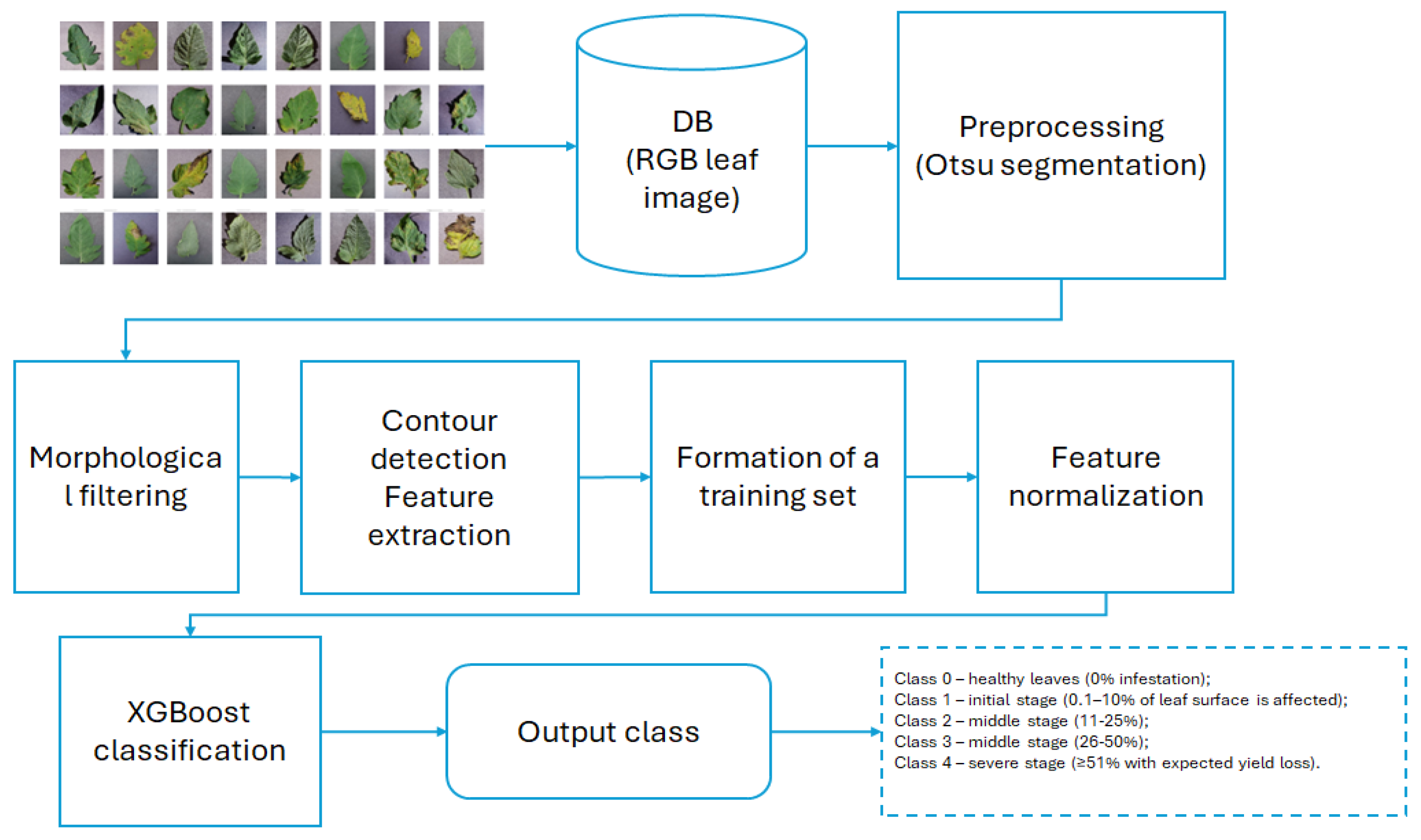
The overall workflow of the proposed system is summarized in Figure 1. Starting from an RGB image of a tomato leaf, the pipeline performs preprocessing, segmentation and morphological filtering; extracts a compact set of texture–geometric features and normalizes them; and finally applies an XGBoost classifier with tuned hyperparameters to predict the late blight severity class.

3.1. Formalization of the Problem

Otsu’s method is an algorithm that automatically determines the optimal global threshold t * , dividing the image into two classes:
Class 1 (background)—intensities I t * .
Class 2 (object)—intensities I < t * .
Otsu seeks a threshold t that maximizes the interclass variance σ b 2 ( t ) , that is, the classes should be as distinguishable as possible [10].
Let P ( i ) is the probability of occurrence for pixels of level i and N is the total number of pixels, i = 0 L 1 P i = 1 . Splitting into two classes for any chosen threshold t of class probabilities:
w 1 t = i = 0 t P i ,       w 2 t = i = t + 1 t P i ,    
Average intensities of classes:
μ 1 t = i = 0 t i P ( i ) w 1 t ,     μ 2 t = i = t + 1 t i P i w 2 t
Overall average:
μ T = i = 0 L 1 i P ( i )
Between-class and within-class variance and between-class variance (goal to maximize):
σ b 2 = w 1 ( t ) w 2 ( t ) μ 1 ( t ) μ 2 ( t ) 2
Intraclass variance (goal to minimize):
σ w 2 t = w 1 t σ 1 2 t + w 2 t σ 2 2 t
Otsu chooses t * that maximizes σ b 2 t or equivalently minimizes σ w 2 t . The final rule:
t * = a rg max t σ b 2 ( t )
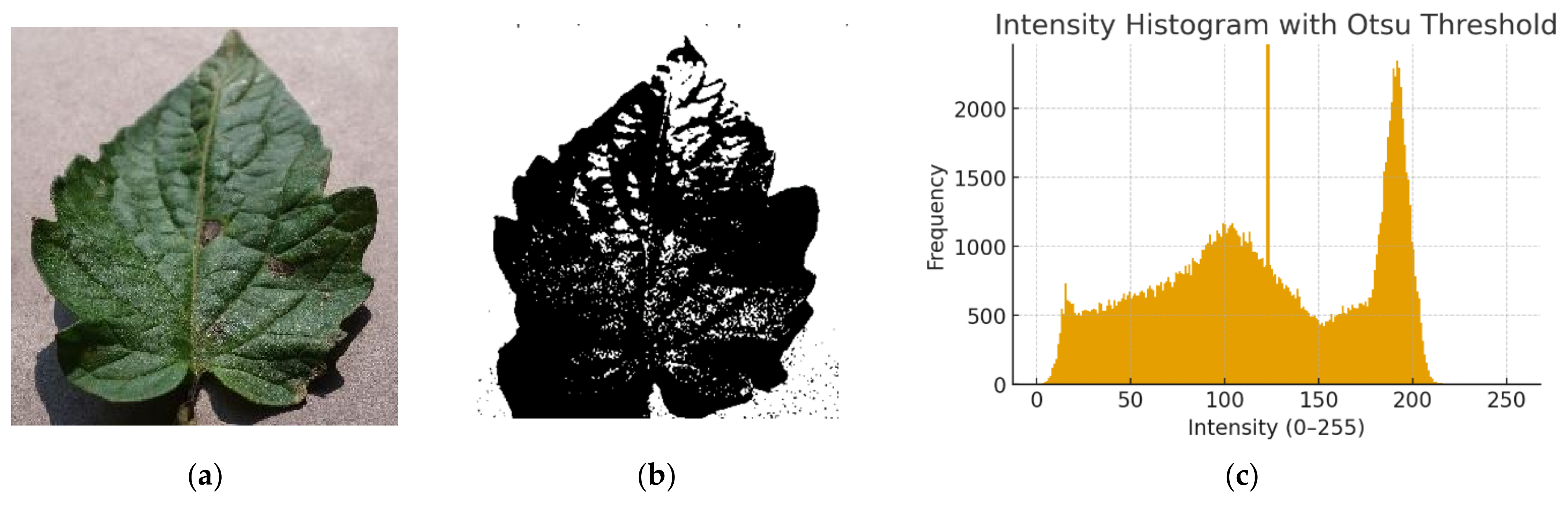
Figure 2 illustrates the image preprocessing and segmentation process using the Otsu thresholding method. The original leaf image is shown in Figure 2a, the resulting binary segmented image in Figure 2b, and the corresponding grayscale intensity histogram with the selected Otsu threshold in Figure 2c.

3.2. Textural and Contour Characteristics

3.2.1. Contrast

This is the standard deviation of pixel brightness. It shows the spread of brightness; the greater the contrast, the greater the difference between dark and light areas. If the contrast is low, the image is too washed out or dark and can be discarded [7].
Root-mean-square deviation:
σ = 1 n i = 1 k ( x i x ¯ ) 2 n i
where x i is the pixel brightness, x ¯ is the average pixel brightness and x ¯ = 1 n i = 1 k x i n i , n i is the pixel number.

3.2.2. Num Contours

This is the number of closed objects found in the binarized image. Let the sets of points C i lie on the boundary of the object and spots [8]:
C i = x , y | I x , y = 1 ˄ x , y ϵ N x , y : I x , y = 0
where N x , y is a set of neighboring points, a point is considered a contour point if it belongs to the object I x , y = 1 , and there is at least one background pixel nearby, I x , y = 0 .
Grouping points into separate contours:
C i = x i 1 , y i 1 , x i 2 , y i 2 , , x i k , y i k
where i is the contour number and, k is the number of points in this contour. The number of contours is the cardinality of the set of all contours found.
The number of contours is the power of the set of all contours found:
K = C i | i = 1,2 , , n

3.2.3. Mean Contour Area

Average area of all contours found. After all contours C 1 , C 2 , , C n have been found, the area is calculated for each [9]. For contour C i , which is represented by the sequence of points from Formula (11), the area is calculated:
A i = 1 2 j = 1 k x i j · y i ( j + 1 ) x i j + 1 · y i j
where k is the number of points in the contours, x i ( k + 1 ) , y i ( k + 1 ) = x i 1 , y i 2 is the closed contour. The average area of all contours if n contours are found, and the average area is calculated:
m = 1 n i = 1 n A i
where A i is square i -th contour.

3.2.4. Standard Contour Area

Formula:
σ A = 1 n i = 1 n A i μ A 2
where A i is the area of the i -th contour and μ A is the average area μ A = 1 n A i .
This shows how much the areas of the contours differ. A larger standard deviation means that there are spots of different sizes.

3.2.5. Mean Contour Perimeter

Formula:
R = 1 n i = 1 n P i
where P i is thelength of the border, i is the contour, and n is the number of contours.
From there
P = i = 1 n x i + 1 x i 2 + y i + 1 y i 2
Average value of perimeters. And the large perimeter of the contour about the complex shape of the spots.

3.2.6. Standard Contour Perimeter

Formula:
σ P = 1 n i = 1 n P i μ P 2
where P i is the perimeter of the i -th contour and μ P is the average perimeter. If the spread of values is large, it means the spots on the leaves have different shapes.

3.2.7. Mean Area to Perimeter Ratio

Formula:
φ = 1 n i = 1 n R i
where R i is the area ratio
Here
R i = A i P i
where A i is the area of the contour and P i is the perimeter of the contour. If R is greater, the closer the shape of the spots is to a circle. If R is smaller, the spots have uneven edges. The geometric texture descriptor extraction is illustrated in Figure 3.

3.2.8. Normalization Signs

The calculation of the area of the object in the image and the allocation of its informative features is carried out as follows [10]:
  • − Contrast;
  • − Num contours;
  • − Mean contour area;
  • − Standard contour area;
  • − Mean contour perimeter;
  • − Standard contour perimeter;
  • − Mean area to perimeter ratio.
These parameters are in each column with an image characteristic that can be extracted from images and used for analysis and recognition in vector values. Combining different features and analyzing them using different image processing and machine learning techniques allows us to create more accurate, faster and more efficient image recognition systems.
After identifying informative features, each feature is normalized in a range from 0 to 1 according to Formula (10) [11]:
I i , j n o r m a l = I i , j I i , j m i n I i , j m a x I i , j m i n
where I i , j n o r m a l is normalized values, I i , j is input values in the column, and I i , j m a x , I i , m i n are the minimum and maximum values of the column.

3.3. XGBoost (Extreme Gradient Boosting)

To improve forecasting accuracy, ensemble methods are used by using multiple primary learners [12]. The basic idea is to train each individual model on multiple datasets and average the results to achieve better model generalization. At the same time, by averaging the results of several models, differences and/or biases in classification can be reduced. In this case, noise, variance, and bias are the causes of the difference between observed and expected values. The ensemble method helps to reduce these variations and deviations.
The most common ensemble methods are bagging and boosting:
Bagging: The main goal of bagging is to reduce the large variance in the model. Decision trees help reduce variance and also have a low variance. Bagging involves creating smaller data sets from a main data set using multiple subsamples. The data from each subset is then placed into separate decision trees, which helps prevent each tree from overfitting the data. The accuracy of the model during bagging depends on the number of decision trees used, and the results are summarized.
Boosting: In boosting, trees are built sequentially, and each subsequent tree tries to reduce the errors of the previous tree. With this approach, weak learners at each stage learn from the mistakes made in previous trees and transfer this information to the new tree. Weak learners exhibit slightly higher accuracy than random guesses, and each one adds small but useful information that can be combined to form a strong learner [14].
The idea of bagging is to form T independent simple algorithms and calculate the output value as an average of the responses from each of them:
a x = 1 T i = 1 T a i ( x )
To emphasize that this approach will be effective if the algorithms’ responses are statistically independent of each other, the constraint can be written as follows:
E a j x · a i ( x ) = 0 ,     i , j : i j
But there are two subtle points in this scheme:
a 1 x ,   a 2 x ,   ,   a T x produce somewhat dependent values (in general, complete independence is impossible to achieve);
They are weighted with the same weighting coefficient 1 T that is, the significance of each is assumed to be equal.
These are very strict conditions and can be considered to be always violated when implementing bagging. This means that potential quality is not achieved when composing algorithms:
a x = t = 1 T α t · b t ( x )
where α t are weights (positive numbers), b t ( x ) are simple algorithms for processing the input vector x . The algorithms produce a real value b t x   ϵ R . In classification problems, this can be the margin value, which for linear algorithms is defined as the scalar product, M = ω , x = ω T · x . That is, the algorithms b t ( x ) produce non-rigid (final) solutions, but a more accurate (intermediate) real value.
When combining algorithms according to Formula (22), weighting coefficients are calculated, and a set of T algorithms is constructed so that a given quality indicator is minimized. For the sake of clarity, the next task will be a binary classification. Then, it is logical to choose the quality indicator as the number of incorrectly classified images [16]:
Q T = i = 1 l M i < 0 = i = 1 l y i · a x i < 0 = i = 1 l y i ·   t = 1 T α t b t x i < 0 a ( x i )
when the offset for the i -th image is less than zero ( M i < 0 ), a classification error has occurred, and the square brackets (Iverson notation) will return 1 . Otherwise, 0 is returned.
There are no hard restrictions on the algorithms b t x i and the weighting coefficients α t . The only thing is that weighting coefficients are usually taken as positive.
It is necessary to optimize both in terms of weights and algorithms:
Q T =   i = 1 l y i · t = 1 T α t b t x i < 0 min α i , b j Q T
But this is a rather complex mathematical problem, so Freund and Shapiro proposed using the following two heuristics:
  • “Greedy” construction of the composition is the search (selection) of the current algorithm b t and the weight factor α t   while fixing the previously found algorithms and weight factors, b 1 x ,     ,   b t 1 ( x ) and α 1 ,   ,   α t 1 . That is, at each step t is calculated as only one weighting coefficient α t and can train only one algorithm b t predominantly on those training set images on which the previous algorithms showed weak results [17].
  • A threshold quality functional in the form of a smooth differentiable loss function, which will allow solving the optimization problem using numerical or analytical methods [18].
These two approaches form the basis of almost all boosting algorithms. That is, it attempts to construct T relatively simple algorithms (classification or regression) and then calculate a weighted sum of their outputs to improve the resulting value according to a chosen quality metric. This is the point of algorithm boosting.
  • Adaptive Boosting (AdaBoost)
AdaBoost applied to binary classification problems with class labels Y =   1 , + 1 . Boosting trains T algorithms and then computes a weighted sum [19]:
a x = i = 1 T α i b i ( x )
Moreover, the search for weights and algorithms is performed according to the “greedy” principle, and all previously found elements, b 1 x ,     ,   b T 1 ( x ) and α 1 ,   ,   α T 1 , are recorded to find the current b T ( x ) and α T . When solving a regression problem, the quality criterion is usually formed using a quadratic loss function:
Q T = 1 2 i = 1 l y i a ( x i ) 2 m i n
That is, the training sample goes through all the objects of X l = x i , y i i = 1 l and calculates the sum of the squares of the errors. If the value of a(x) is written into Formula (26), it will change as follows [20]:
Q T = 1 2 i = 1 l y i j = 1 T α j b j x i 2 = 1 2 i = 1 l y t j = 1 T 1 b j ( x i ) b T ( x i ) S i , T 1 2
Here it can be noted that, firstly, in linear regression problems, the factors α j = 1 can be discarded, since they only determine the scale of the output responses of the algorithms. This scale can be formed by the algorithm itself, b J ~ x = α i b i ( x ) . And secondly, given fixed previous weights and algorithms, at step T the residual values are minimized:
S i , T 1 = y i j = 1 T 1 b j x i ,       i = 1,2 , , l
It is necessary to decide on the choice of the family of algorithms { b j x i } for the regression problem. A common case is decision trees, as in classification problems. In general, boosting over crucial trees is a classic and the most common way of using it. Although, there are other algorithm families to choose from, for example, a set of linear algorithms, etc. The main thing is that these algorithms can be formed and then used relatively quickly (from a computational point of view) [21].
Thus, if decision trees are chosen, then in regression problems, with a quadratic loss function, the leaves store the average values of the target labels y i of the objects that fall into them. If the M objects R v = x i , y i i = 1 M of the training sample have reached some leaf node, then the optimal value for their description can be found from the equation:
Q = 1 2 i e R v y i c 2 m i n ,     d Q d c = i e R v y i c = 0  
Here, c = 1 R v i e R v y i .
With a different loss function, the value of c can be calculated differently. As a result, the pseudocode of the AdaBoost algorithm as applied to regression problems will look like this:
Input: training sample X l   and parameter T (number of algorithms in the composition). Output: set of basic algorithms b 1 x ,     ,   b T ( x ) [22].
Initialization of residues: S i , 0 = y i , i = 1,2 , , l ;
For all t = 1,2 , , T ;
Find the best current algorithm using the rule: b t = a rg min b l   Q t ,
Update balances: S i , t = S i , t 1 b t ( x i ) .
Different problems use different loss functions in the composition quality functional:
Q T α , b = i = 1 l L ( a x , y i ) min α , b   Q T
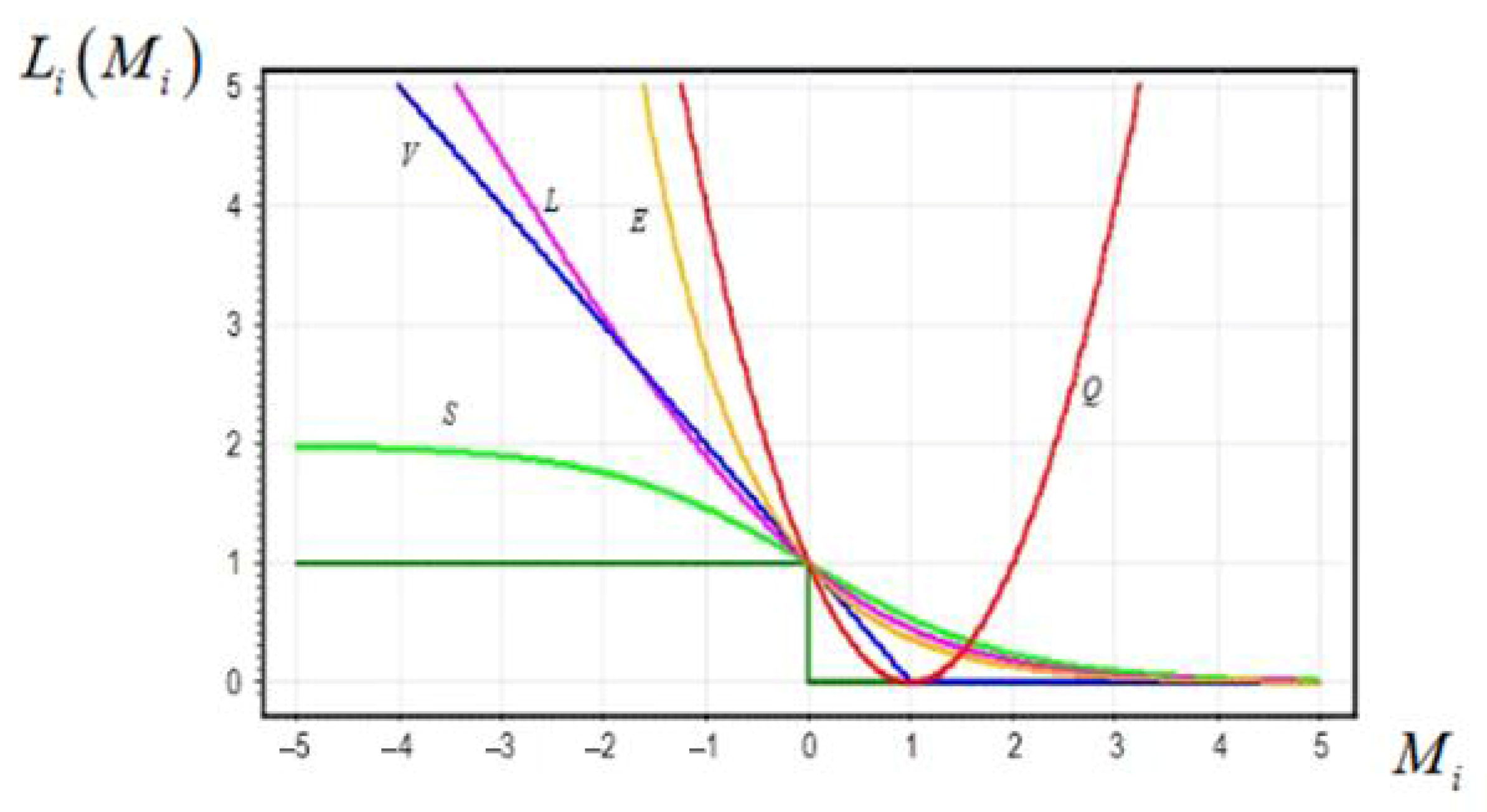
according to the training sample X l = x i , y i i = 1 l . Thus, in a binary classification problem, the AdaBoost algorithm uses an exponential loss function, and in a regression problem, it uses a quadratic loss function. Other loss functions allow us to obtain other well-known boosting algorithms in Figure 4:
  • E M = e x p ( M ) —exponential (AdaBoost);
  • L M = log 2 1 + e M —logarithmic (LogitBoost);
  • Q M = 1 M 2 —quadratic (GentleBoost);
  • G M = e x p ( c M · ( M + s ) ) —Gaussian (BrownBoost).
One can come up with many other functions for developing (synthesizing) new boosting algorithms [23]. A universal boosting algorithm that would work with an arbitrary smooth and differentiable loss function is called gradient boosting. Gradient boosting has become one of the standard tools for trying to solve a particular machine learning problem. The principles of gradient boosting are a fragment of its derivation from Formula (31),
a x = i = 1 T α i , b i ( x )
and the choice of the quality functional for searching for weights α i   and specific algorithms b i ( x ) . It can be written in general form through some loss function L ( a x i , y i ) [24].
Q α , b = i = 1 l L t = 1 T 1 α t b t ( x i ) + α b x i , y i f T 1 , i f T , i min α , b   Q ( α , b )
Here, a composition is immediately written through ( T 1 ) already known algorithms (found in the previous ( T 1 ) steps) and the current b x i with some (still unknown) weight α . These two elements must be found here from the condition of the minimum of the functional Q ( α , b ) . What is implemented here is a “greedy” strategy for searching algorithms: all previously found algorithms b 1 , ,   b T 1 and weight coefficients α 1 , , α T 1 are fixed and no longer change [25]. The outputs of the composition are denoted according to ( T 1 ) algorithms for each pattern x i of the training sample by the vector f T 1 f T 1.1 , f T 1.2 , , f T 1 , l T . And the outputs for all T algorithms are through the vector f T f T , 1 , f T , 2 , , f T , l T . And at the next step, T must choose a vector f T , that would reduce the value of the quality functional Q ( α , b ) compared to the previous vector f T 1 . The description of the operation of the gradient algorithm and the gradient of the loss function:
g i = L ( f T 1 , i , y i ) f T 1 , i = L f T 1 , i , y i ,     i = 1,2 , , l
That the correction of the i -th component can be written as follows:
f T , i = f T 1 , i α g i
In the formula (according to the composition of the algorithms), this same adjustment looks like this:
f T , i = f T 1 , i + α b ( x i )
The similarities are obvious. And since the coefficient α > 0 , then the algorithm b ( x i ) at the current step T should produce values as close as possible to the antigradient of the loss:
b T = a rg min b i = 1 l b x i + g i 2
Here, a quadratic function is used as a measure of the closeness of the i -th values, and everything is summed up over the training sample; decision trees for regression problems often use this criterion by default.
Find the best algorithm b T at step T , knowing the gradient of the loss function and solving the least squares problem. And the last thing that remains is to calculate (find) the weighting coefficient α T . Since a general problem with an arbitrary loss function, the search for this weighting coefficient is reduced to the following one-dimensional optimization problem:
α T = a rg min α > 0 i = 1 l L f T 1 , i + α b T x i , y i
It can be solved fairly quickly using numerical methods. Modern optimization methods can easily handle this (for example, the bisection method).
Input: training sample X l and parameter T (number of algorithms in the composition). Output: a set of base algorithms b 1 x , , b T ( x ) and weights α 1 , , α T
Initialization: f i = 0 , i = 1 , , l
For all t = 1 , , T ;
Find the best current algorithm that approximates the antigradient: b t = a rg min b i = 1 l b x i + g i 2 ;
Find the weighting coefficient: Formula (37);
Update the vector of values on the sample objects: f i = f i + α t b t x i , i = 1,2 , , l .

3.4. Grid Search

In the grid of hyperparameters, there are J hyperparameters, each given a finite set of values [26]:
Θ j = θ j , 1 , , θ j , m j ,   j = 1 , , J
The Cartesian product forms a grid:
Θ = j = 1 J m j ,   Θ = Θ 1 · , , · Θ J
Training operator (abstract): Let A ( D ; θ ) is an operator that, given data D and a setting θ Θ , returns a trained model f θ .
Evaluation metric: Let S ( f , D v a l ) is a scalar quality metric (the higher the better) calculated on the validation data D v a l .
K fold (stratified) cross-validation: The training set D is split into K disjoint folds of indices S 1 , , S K (class proportions are preserved during stratification). For each θ Θ a CV score is determined [27]:
S C V ^ θ = 1 K k = 1 K S A D S k , θ , S k
The model is trained on D S k and tested on S k .
Hyperparameter selection criterion: Finds the grid point that maximizes the average CV score:
θ * = a r g max θ Θ S C V ^ θ
The final model: After selecting θ * the model is retrained on all available training data:
f θ * = A ( D , θ * )
Counting the number of training runs and the complexity and the number of training runs for K -fold:
N f i t s = Θ · K
and time costs are scaled as: O ( Θ K t i m e _ t r a i n ( θ ) ) .
In this work, XGBoost is used to classify tomato leaf images into five levels of late blight damage. Each data instance is a vector of texture descriptors that forms the input space X. The model is trained on the labeled sample and then predicts the probability that pixels or images belong to the corresponding disease class.

3.5. Evaluation Metrics

To evaluate the effectiveness of the proposed approach based on the XGBoost algorithm, standard machine learning indicators are used: accuracy, precision, responsiveness, and F1 score. These indicators allow us to comprehensively assess the accuracy of the classification [28,35].
The metrics are based on four possible classification outcomes:
  • T P (True Positive)—a correctly identified diseased tomato leaf (the algorithm correctly classified the disease);
  • T N (True Negative)—a correctly identified healthy tomato leaf (the algorithm correctly classified it as “healthy”);
  • F P (False Positive)—a healthy leaf is mistakenly identified as diseased (false positive);
  • F N (False Negative)—a diseased leaf is mistakenly identified as healthy (missed disease).
  • Accuracy (Overall accuracy)
Shows the proportion of correctly classified examples [29,36]:
A c c u r a c y = T P + T N T P + T N + F P + F N
  • Precision (Positive Class Accuracy)
Characterizes the reliability of the prediction:
P r e c i s i o n = T P T P + F N
  • Recall (Recall, Sensitivity)
Determines which part was correctly recognized:
R e c a l l = T P T P + F N
  • F1-score (Balanced Metric)
Allows simultaneous consideration of precision and recall:
F 1 = 2 · P r e c i s i o n · R e c a l l P r e c i s i o n + R e c a l l

4. Results

The XGBoost algorithm was proposed as the primary classifier, allowing for the effective classification of tomato leaf condition classes based on a combination of textural and contour-geometric features: contrast, number of contours, mean and standard values of contour areas and perimeters, and area-to-perimeter ratios. To form the sample, images of healthy and diseased leaves (by stage) were collected and labeled, after which the specified descriptors were extracted and normalized.

4.1. Formation of Input Data

For this study, we created our own dataset of tomato leaf images. RGB photographs were acquired in greenhouse conditions in Uzbekistan using a Samsung Galaxy S22 Ultra (Samsung, South Korea) smartphone. The main camera has a 108 MP sensor (f/1.8) with a maximum photo resolution of 12,000 × 9000 pixels. Additional cameras include a 12 MP ultra-wide and two 10 MP telephoto lenses (3× and 10× optical zoom). Natural illumination was used, with approximate brightness ranging between 400 and 600 lux. The images contain single leaves on heterogeneous backgrounds (soil, sky, and greenhouse equipment) and exhibit realistic variability in focus, angle, scale, and leaf orientation.
Each image was annotated by an agronomist into one of five late blight severity classes according to the percentage of visibly affected leaf area:
-
Class 0—healthy leaf (0% infection);
-
Class 1—initial stage (0.1–10% of the leaf surface affected);
-
Class 2—moderate stage (11–25%);
-
Class 3—middle stage (26–50%);
-
Class 4—severe stage (≥51% with expected yield loss).
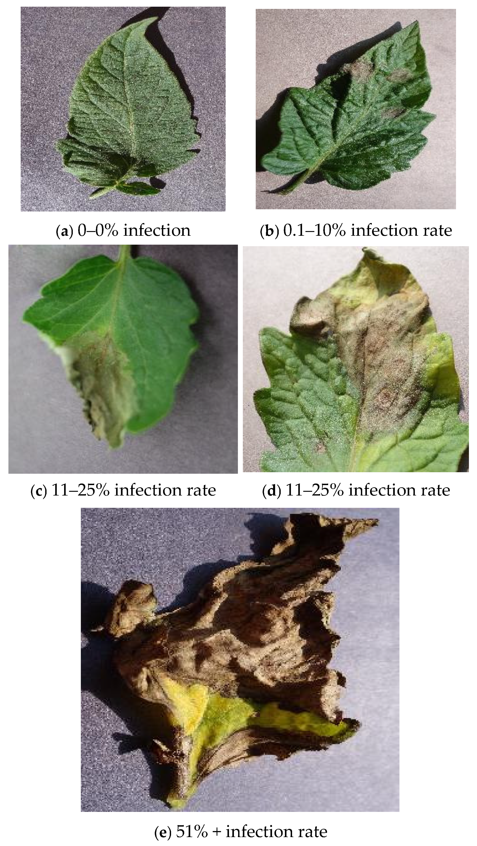
Late blight (Phytophthora infestans) is a major tomato disease in Uzbekistan, significantly affecting local crop yields and potentially reducing them by 60–70% if not detected at an early stage. Given the severity of its impact on Uzbek tomato production, traditional diagnostic methods, including visual inspection and laboratory testing, are time-consuming and rely heavily on specialist expertise, which limits their practicality for large-scale production systems. In total, the dataset contains 5245 images of tomato leaves. To evaluate the model, the data was randomly divided into training and test parts in an 80/20 ratio with class stratification, resulting in 4129 training images and 1049 test images. This dataset is used throughout the experimental section to train, validate, and test all the models being compared. Some example images from the dataset are shown in Figure 5.
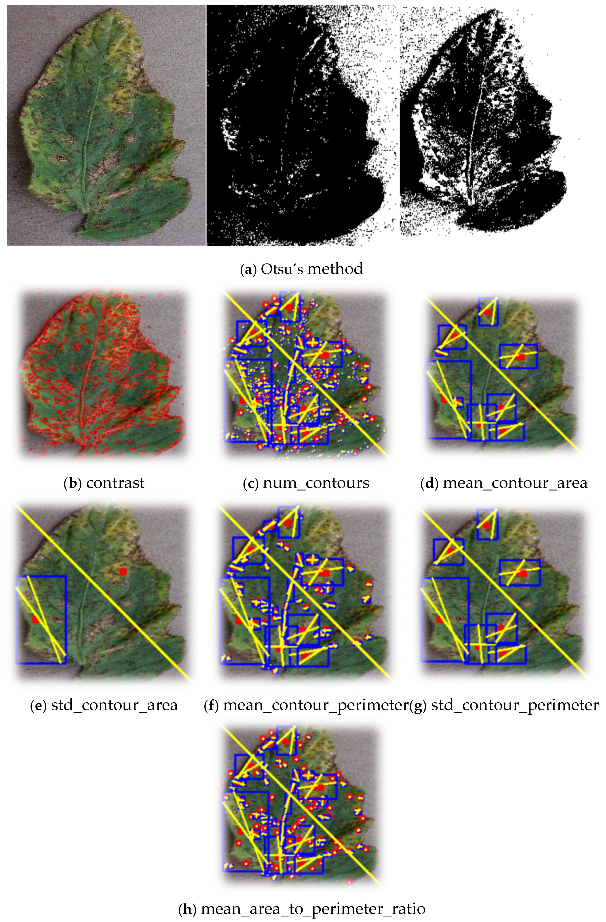
The next step involves pre-processing the image using Otsu’s method to separate areas of the leaf by intensity and highlight the affected areas as illustrated in Figure 6.

4.2. Formation of a Vector Training Sample

As a result of processing the images of tomato leaves, a training sample was formed for the T n m l , in Table 1, containing both textural and geometric features, where T is the training sample, n are the features, s   are the objects, and K   are the classes. This sample is further used for training and testing machine learning models.
Each record of the training sample is a feature vector that includes the following parameters.
  • Signs
  • Textural and contour characteristics:
x 1 = contrast;
x 2 = num_contours;
x 3 = mean_contour_area;
x 4 = std_contour_area;
x 5 = mean_contour_perimeter;
x 6 = std_contour_perimeter;
x 7 = mean_area_to_perimeter_ratio.
Objects:
S 1 = healthy leaf;
S 2 = 0.1–10% (initial stage);
S 3 = 11–25% (moderate stage);
S 4 = 26–50% (middle stage);
S 5 = more 51% (severe stage with loss of yield).
Classes:
K 1 = 0–0% infection.
K 2 = 1–0.1–10% infection rate.
K 3 = 2–11–25% infection rate.
K 4 = 3–26–50% infection rate.
K 5 = 4–51% + infection rate.

4.3. Normalization of Training Sample Features

To ensure the correct functioning of the machine learning model, all numerical features of the training sample were subjected to a normalization procedure. This operation is necessary because the features have different ranges of values. The use of normalization allows:
  • Reduce the influence of features with large numerical ranges on the model error function;
  • Speed up the convergence of gradient learning methods;
  • Improve the robustness and accuracy of classification.
  • Normalization method
In this work, linear normalization (Min–Max Scaling) is used, which transforms the values of each feature x   to the range [ 0,1 ] as given in Table 2:
  • Using normalized data:
After normalization, all features form a single vector X i = [ x 1 , x 2 , , x n ] , which is fed to the classifier as input. This approach allows the model to equally consider both fractal and textural–geometric characteristics without a bias toward features with larger initial ranges.

4.4. Classification

This study implemented an experiment to classify images of tomato leaves using the XGBoost algorithm.
  • Description of the experiment:
The XGBoost classification algorithm was trained on 80% of the sample, and the remaining 20% were used for testing;
Grid Search;
Model evaluation (metric);
Confusion matrix (test).
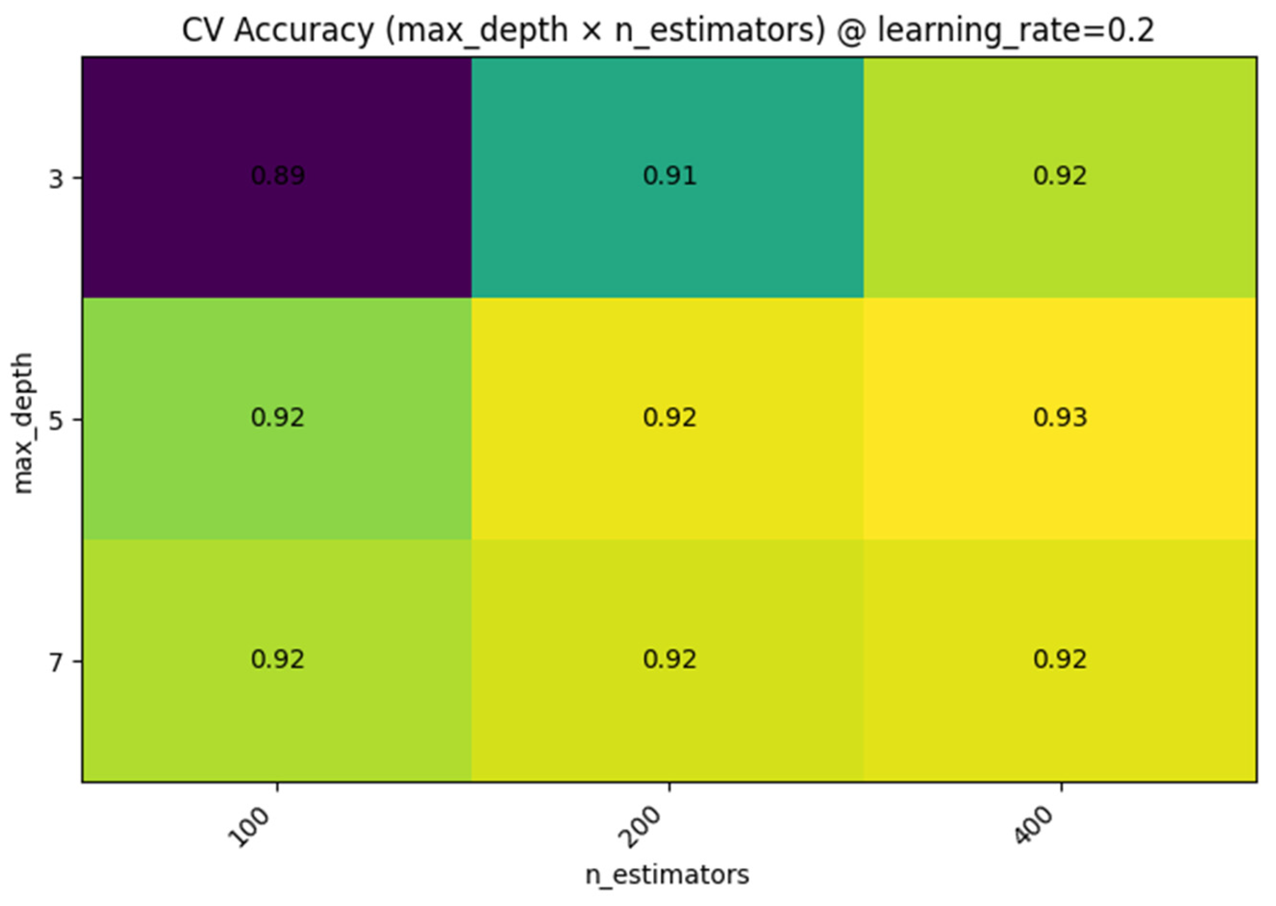
Figure 7 shows a heatmap of the cross-validation accuracy (CV Accuracy) when changing the max_depth and n_estimators hyperparameters for XGBoost; the best result (0.93) is achieved with max_depth = 5 and n_estimators = 400.
The results in Table 3 show that the proposed model maintains a high and balanced performance across all five severity classes. The lowest F1-score (0.90) is obtained for class two, which corresponds to the visually ambiguous transition between early and middle stages of infection.
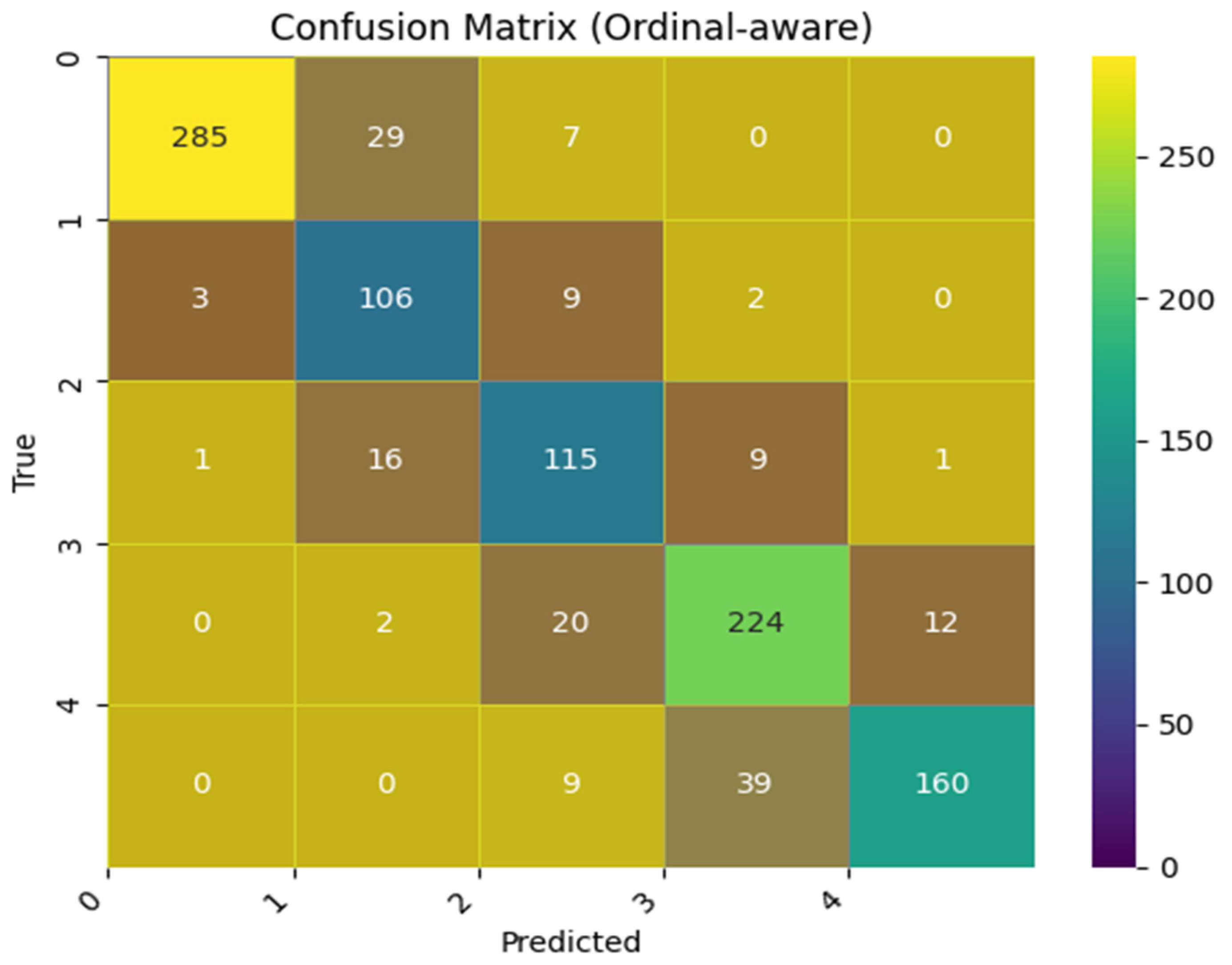
The classification performance of the proposed model is illustrated in Figure 8, which presents the confusion matrix summarizing the prediction results across different classes.
After classification, each test sample was assigned to one of five tomato leaf disease severity classes. The results demonstrated the high accuracy of the XGBoost model and consistent discrimination between healthy and diseased samples at all stages of late blight development.
  • Comparison with existing methods
We compare our CNN method (Siamese-CNN), the EfficientNetV2 + Swin hybrid model, and classical algorithms (SVM, Random Forest, k-NN, Logistic Regression) using the same data partitioning and the same metrics (accuracy, macro-F1, F1 per class), as well as measuring inference time and peak CPU memory consumption in Table 4. Comparisons with results from other studies are provided only as a guide, as they used different datasets and experimental protocols.
The proposed XGBoost model demonstrates an optimal balance between accuracy and computational efficiency. While achieving classification quality similar to neural network methods, it operates faster and requires significantly fewer resources, making it suitable for implementation in local and mobile plant health monitoring systems.
The architecture in Table 5 reflects the classic structure of an image analysis pipeline. First, leaf segmentation is performed using Otsu’s method and morphological refinement. Then, the contours of the diseased areas are extracted, and the texture and geometric features are identified, normalized, and fed into the conservative XGBoost classifier. The model runs on a CPU, does not require a GPU, and is suitable for use in the field or on simple computer plants.

5. Analysis and Discussion

The optimized XGBoost model on texture–geometric descriptors demonstrated accuracy = 0.93 on the test set and CV-Accuracy ≈ 0.92 (5-fold GridSearchCV), which indicates the stability of the evaluation. The coincidence of macro-F1 = 0.93 and weighted-F1 = 0.93 confirms the uniformity of quality with moderate class imbalance. By class: 0—0.97/0.97/0.97; 1—0.91/0.93/0.92; 2—0.95/0.85/0.90; 3—0.91/0.95/0.93; and 4—0.92/0.92/0.92 (precision/recall/F1). The confusion matrix shows typical 1↔2 and 3↔4 biases that are characteristic of the ordinal severity scale; isolated 0→3 biases are associated with vein shadows and microtexture. Ablations confirm the contribution of the components: without mean/std perimeter −1.2 p.p., without num_contours −0.8 p.p., and without GridSearch −1.5 p.p. Therefore, perimeter features and hyperoptimization are critical for distinguishing between medium/heavy stages. The pipeline is CPU-only, low-memory, and interpretable (importance/SHAP), facilitating on-farm implementation; the main reserves remain increasing class two recall and reducing 3↔4 bias.
The obtained results confirm that the combination of carefully constructed texture–geometric descriptors with XGBoost provides practically significant quality with minimal resources and high interpretability. On the ordinal scale of late blight severity, the model demonstrates uniform metrics for most classes; characteristic errors arise at “borderline” stages (1↔2, 3↔4), where differences in the area and heterogeneity of lesions are small and partially masked by illumination variations. Perimeter features (mean/std perimeter) make a key contribution to distinguishing the moderate/severe stages, which is confirmed by ablations. Comparison with DL approaches from the literature reveals the expected trade-off: we give up a few percentage points in maximum accuracy, but gain in speed, memory, and ease of implementation (CPU-only), which is critical for greenhouse/field scenarios. The limitations are related to domain shift, subjectivity of lesion proportion labeling, and ignoring the class order during the training stage. Practically significant areas of development are ordinal-aware learning, probability calibration, and the expansion of the set of local features to increase completeness at early stages.

6. Conclusions

In this article, we presented an XGBoost–based method for assessing the degree of late blight on tomato leaves using a compact set of textural and geometric descriptors. This approach is based on the global determination of the Otsu threshold and morphological filtering for segmentation of leaf and lesion areas, followed by the identification of seven interpretable features describing the contrast, number, area and perimeter of contours, as well as their ratio. The hyperparameters of the XGBoost classifier are adjusted using GridSearchCV and K-fold cross-validation. Based on an independent test set of images of tomato leaves, the model achieved an overall accuracy of 0.93 and an F1 macro score of 0.93 points with balanced performance across all five hazard classes.
The proposed solution is characterized by low weight, processor compatibility, and ease of integration into existing monitoring systems. Analyzing the importance of characteristics and visualizing lesion contours makes solutions transparent to agronomists and greenhouse operators, which is crucial for practical applications. At the same time, there are still some limitations: the boundaries between neighboring severity levels are inherently fuzzy, and the model may be sensitive to strong shifts in area (camera type, lighting, and grade).
Further work will focus on three areas. First, we plan to include the ordinal number of the severity scale directly into the loss detection function or decision-making strategy of the classifier [37,38]. Secondly, we intend to expand the framework to images containing multiple leaves and combine predictions at the object level within a single frame. Third, we are considering the possibility of extending the feature set with additional color and fractal descriptors and testing this approach on datasets collected in other regions and seasons to further improve reliability and generalization. We also want to expand the possibilities of assessing not only the leaves of greenhouse tomatoes affected by late blight (Phytophthora infestans) but also other plant diseases and various types of crops. This extension will allow a comprehensive assessment of the generalizing ability of the model and its reliability in various growing conditions, regions, and varieties. The purpose of these steps is to ensure that the proposed method is effectively applied to a wider range of agricultural scenarios beyond the current dataset.

Author Contributions

Methodology, A.K., J.K., K.S., I.S. and B.A.; software, A.K. and B.A.; validation P.A., R.O. and B.A.; formal analysis, A.K., B.A., J.K. and K.S.; resources, P.A., R.O., I.S. and K.S.; data curation, B.A., J.K., A.K., R.O. and P.A.; writing—original draft, B.A. and A.K.; writing—review and editing, B.A., J.K. and A.K.; supervision, K.S. and A.K.; project administration, A.K. and J.K. All authors have read and agreed to the published version of the manuscript.

Funding

This research was supported by the project “AL-9424104925-R1”, funded by the Agency for Innovative Development under the Ministry of Higher Education, Science and Innovation of the Republic of Uzbekistan.

Institutional Review Board Statement

Not applicable.

Informed Consent Statement

Not applicable.

Data Availability Statement

The data presented in this study are available on request from the corresponding author.

Acknowledgments

The authors would like to thank the editor and anonymous referees for the constructive comments in improving the contents and presentation of this paper.

Conflicts of Interest

The authors declare no conflicts of interest.

References

  1. Chen, Z.; Ding, Z.; Meng, Q. The impact of national modern agriculture demonstration zones on rural household development resilience. Int. Rev. Econ. Financ. 2025, 104, 104652. [Google Scholar] [CrossRef] [Scilit]
  2. Halder, R.K.; Lima, M.A.; Uddin, M.N.; Islam, A.; Saha, A. Integrated feature selection-based stacking ensemble model using optimized hyperparameters to predict breast cancer with smart web application. Clin. eHealth 2025, 8, 146–161. [Google Scholar] [CrossRef] [Scilit]
  3. Su, Q.; Chen, L.; Qian, L. Optimization of big data analysis resources supported by XGBoost algorithm: Comprehensive analysis of industry 5.0 and ESG performance. Meas. Sens. 2024, 36, 101310. [Google Scholar] [CrossRef] [Scilit]
  4. Liu, X. Enhanced prediction of karst spring discharge using a hybrid LSTM-XGBoost model optimized with grid search. Mach. Learn. Appl. 2025, 22, 100740. [Google Scholar] [CrossRef] [Scilit]
  5. Wu, S.; Ding, S.; Geng, L.; Chen, Z.; Han, S.; Zhou, L. A grid search-based optimal trajectory planning approach for automatic berthing of underactuated unmanned surface vehicles. Ocean Eng. 2025, 336, 121707. [Google Scholar] [CrossRef] [Scilit]
  6. Günen, M.A.; Atasever, U.H. Remote sensing and monitoring of water resources: A comparative study of different indices and thresholding methods. Sci. Total Environ. 2024, 926, 172117. [Google Scholar] [CrossRef] [Scilit]
  7. Yomtako, S.; Kume, S.; Watanabe, H.; Kuribayashi, A.; Nakamura, S.; Imaizumi, A.; Tomisato, H.; Nomura, Y.; Taguchi, M.; Oki, A.; et al. Dynamic contrast-enhanced magnetic resonance imaging for distinguishing vital and non-vital teeth in jaw lesions: A pilot study. Oral Surg. Oral Med. Oral Pathol. Oral Radiol. 2025, 141, 239–244. [Google Scholar] [CrossRef] [Scilit]
  8. Kos, A.; Majek, K.; Belter, D. Enhanced lightweight detection of small and tiny objects in high-resolution images using object tracking-based region of interest proposal. Eng. Appl. Artif. Intell. 2025, 153, 110852. [Google Scholar] [CrossRef] [Scilit]
  9. Liu, T.; Dong, K.; Song, Y.; Zhang, G.; Li, J. Real-time spectral target detection based on saliency and edge contour fusion. Opt. Laser Technol. 2025, 192, 113951. [Google Scholar] [CrossRef] [Scilit]
  10. Pitkäkangas, V. Rectangular partition for n-dimensional images with arbitrarily shaped rectilinear objects. Heliyon 2024, 10, e35956. [Google Scholar] [CrossRef] [Scilit]
  11. Dai, J.-C.; Wang, D.-S.; Tang, W.-J.; Zou, Y.-H.; Hui, Y.-X.; Zhang, Y.-J. Parameter-normalized probabilistic seismic demand model considering the structural design strength for structural response assessment. Soil Dyn. Earthq. Eng. 2024, 187, 109023. [Google Scholar] [CrossRef] [Scilit]
  12. Gao, X.; Wang, X.; Cao, L.; Guo, H.; Chen, W.; Zhai, X. XT-SECA: An Efficient and Accurate XGBoost-Transformer Framework for Urban Functional Zone Classification. ISPRS Int. J. Geo-Inf. 2025, 14, 290. [Google Scholar] [CrossRef] [Scilit]
  13. Zhang, L.; Huang, Z. Spectral data analysis based on bagging stochastic configuration networks. Infrared Phys. Technol. 2024, 143, 105609. [Google Scholar] [CrossRef] [Scilit]
  14. Shuaib, S.E.; Riyapan, P.; Muangprathub, J. Formal concept views for explainable boosting: A lattice-theoretic framework for Extreme Gradient Boosting and Gradient Boosting Models. Intell. Syst. Appl. 2025, 27, 200569. [Google Scholar] [CrossRef] [Scilit]
  15. Xo‘jamqulov, A.; Adirov, T.; Karimov, B.; Umarov, U. Exploring the Efficacy of Heteroscedasticity Reduction Methods in Multifactor Regression Models Using Python. In Internet of Things, Smart Spaces, and Next Generation Networks and Systems; ruSMART NEW2AN 2024 2024. Lecture Notes in Computer Science; Koucheryavy, Y., Aziz, A., Eds.; Springer: Cham, Switzerland, 2026; Volume 15555. [Google Scholar] [CrossRef] [Scilit]
  16. Imani, M.; Beikmohammadi, A.; Arabnia, H.R. Comprehensive Analysis of Random Forest and XGBoost Performance with SMOTE, ADASYN, and GNUS Under Varying Imbalance Levels. Technologies 2025, 13, 88. [Google Scholar] [CrossRef] [Scilit]
  17. Wang, J.; Cerrone, C.; Golden, B. Carousel greedy algorithms for the minimum stretch spanning tree problem. Comput. Oper. Res. 2025, 184, 107229. [Google Scholar] [CrossRef] [Scilit]
  18. Yu, H.; Xiao, H.; Gu, X. Integrating species distribution and piecewise linear regression model to identify functional connectivity thresholds to delimit urban ecological corridors. Comput. Environ. Urban Syst. 2024, 113, 102177. [Google Scholar] [CrossRef] [Scilit]
  19. Hussain, S.S.; Zaidi, S.S.H. AdaBoost Ensemble Approach with Weak Classifiers for Gear Fault Diagnosis and Prognosis in DC Motors. Appl. Sci. 2024, 14, 3105. [Google Scholar] [CrossRef] [Scilit]
  20. Sui, Q.; Ghosh, S.K. Active Learning for Stacking and AdaBoost-Related Models. Stats 2024, 7, 110–137. [Google Scholar] [CrossRef] [Scilit]
  21. Cheng, T.; Xiao, J. Cost-constrained feature selection using gradient boosting decision tree. Eng. Appl. Artif. Intell. 2025, 162, 112751. [Google Scholar] [CrossRef] [Scilit]
  22. Sayeri, R.; Barzegar, B.; Bozorgi rad, Y.; Mikaeilvand, N.; Najaran, M.H.T. Evolutionary AdaBoost ensemble: A machine learning framework for depression detection. Mach. Learn. Appl. 2025, 22, 100748. [Google Scholar] [CrossRef] [Scilit]
  23. Pittayapong, S.; Hametner, S.; Bachratá, B.; Endmayr, V.; Bogner, W.; Höftberger, R.; Grabner, G. Synthesized myelin and iron stainings from 7T multi-contrast MRI via deep learning. NeuroImage 2025, 318, 121417. [Google Scholar] [CrossRef] [Scilit]
  24. Ganiev, J.; Kim, D.-W.; Bae, S.-H. Neural-NGBoost: Natural gradient boosting with neural network base learners. ICT Express 2025, 11, 974–980. [Google Scholar] [CrossRef] [Scilit]
  25. Pichi, F.; Strazzullo, M. Deflation-based certified greedy algorithm and adaptivity for bifurcating nonlinear PDEs. Commun. Nonlinear Sci. Numer. Simul. 2025, 149, 108941. [Google Scholar] [CrossRef] [Scilit]
  26. Spence, M.A. Using history matching to speed up management strategy evaluation grid searches. Can. J. Fish. Aquat. Sci. 2025, 82, 1–14. [Google Scholar] [CrossRef] [Scilit]
  27. Vhatkar, M.S.; Mahajan, P.S.; Raut, R.D.; Cheikhrouhou, N.; Ghoshal, S. Optimized hyperparameters for retail sales forecasting using grid search. Eng. Appl. Artif. Intell. 2025, 158, 111472. [Google Scholar] [CrossRef] [Scilit]
  28. Ratanpaul, V.; Hands, P.; Stockmann, R. Metrics to assess pulse grains for protein enrichment potential in air classification. Food Res. Int. 2025, 214, 116505. [Google Scholar] [CrossRef] [Scilit]
  29. Zimney, K.; Turbak, T.; Fjeldheim, E. Differences in tactile grid localization accuracy between people with back pain compared to individuals without pain. Musculoskelet. Sci. Pract. 2025, 79, 103394. [Google Scholar] [CrossRef] [Scilit]
  30. Rakhimovich, M.A.; Kadirbergenovich, K.K.; Rakhmovich, O.U.; Rustem, J. A New Type of Architecture for Neural Networks with Multi-connected Weights in Classification Problems. In 12th World Conference Intelligent System for Industrial Automation (WCIS-2022); Aliev, R.A., Yusupbekov, N.R., Kacprzyk, J., Pedrycz, W., Babanli, M.B., Sadikoglu, F.M., Turabdjanov, S.M., Eds.; WCIS 2022 Lecture Notes in Networks and Systems; Springer: Cham, Switzerland, 2024; Volume 718. [Google Scholar] [CrossRef] [Scilit]
  31. Thuseethan, S.; Vigneshwaran, P.; Charles, J.; Wimalasooriya, C. Siamese Network-Based Lightweight Framework for Tomato Leaf Disease Recognition. Computers 2024, 13, 323. [Google Scholar] [CrossRef] [Scilit]
  32. Sun, Y.; Ning, L.; Zhao, B.; Yan, J. Tomato Leaf Disease Classification by Combining EfficientNetv2 and a Swin Transformer. Appl. Sci. 2024, 14, 7472. [Google Scholar] [CrossRef] [Scilit]
  33. Osmenaj, Z.; Tseliki, E.-M.; Kapellaki, S.H.; Tselikis, G.; Tselikas, N.D. From Pixels to Diagnosis: Implementing and Evaluating a CNN Model for Tomato Leaf Disease Detection. Information 2025, 16, 231. [Google Scholar] [CrossRef] [Scilit]
  34. Nishankar, S.; Mithuran, T.; Thuseethan, S.; Sebastian, Y.; Yeo, K.C.; Shanmugam, B. TOM-SSL: Tomato Disease Recognition Using Pseudo-Labelling-Based Semi-Supervised Learning. AgriEngineering 2025, 7, 248. [Google Scholar] [CrossRef] [Scilit]
  35. Abdusalomov, A.; Umirzakova, S.; Kutlimuratov, A.; Mirzaev, D.; Dauletov, A.; Botirov, T.; Zakirova, M.; Mukhiddinov, M.; Cho, Y.I. Lightweight UAV-Based System for Early Fire-Risk Identification in Wild Forests. Fire 2025, 8, 288. [Google Scholar] [CrossRef] [Scilit]
  36. Mamadmurodov, A.; Umirzakova, S.; Rakhimov, M.; Kutlimuratov, A.; Temirov, Z.; Nasimov, R.; Meliboev, A.; Abdusalomov, A.; Im Cho, Y. A Hybrid Deep Learning Model for Early Forest Fire Detection. Forests 2025, 16, 863. [Google Scholar] [CrossRef] [Scilit]
  37. Madrakhimov, S.; Makharov, K.; Khurramov, A. On the Transparency of Decision-Making in Classification by Precedents With Fuzzy Descriptions. IEEE Access 2025, 13, 173656–173664. [Google Scholar] [CrossRef] [Scilit]
  38. Rakhimovich, A.M.; Kadirbergenovich, K.K.; Ishkobilovich, Z.M.; Kadirbergenovich, K.J. Logistic Regression with Multi-Connected Weights. J. Comput. Sci. 2024, 20, 1051–1058. [Google Scholar] [CrossRef] [Scilit]
Figure 1. Workflow of the proposed XGBoost–based tomato leaf disease recognition system.
Agriengineering 08 00098 g001
Figure 2. Otsu’s method. (a) Original image, (b) Binary segmentation result obtained using Otsu thresholding; (c) Intensity histogram with Otsu Threshold.
Agriengineering 08 00098 g002
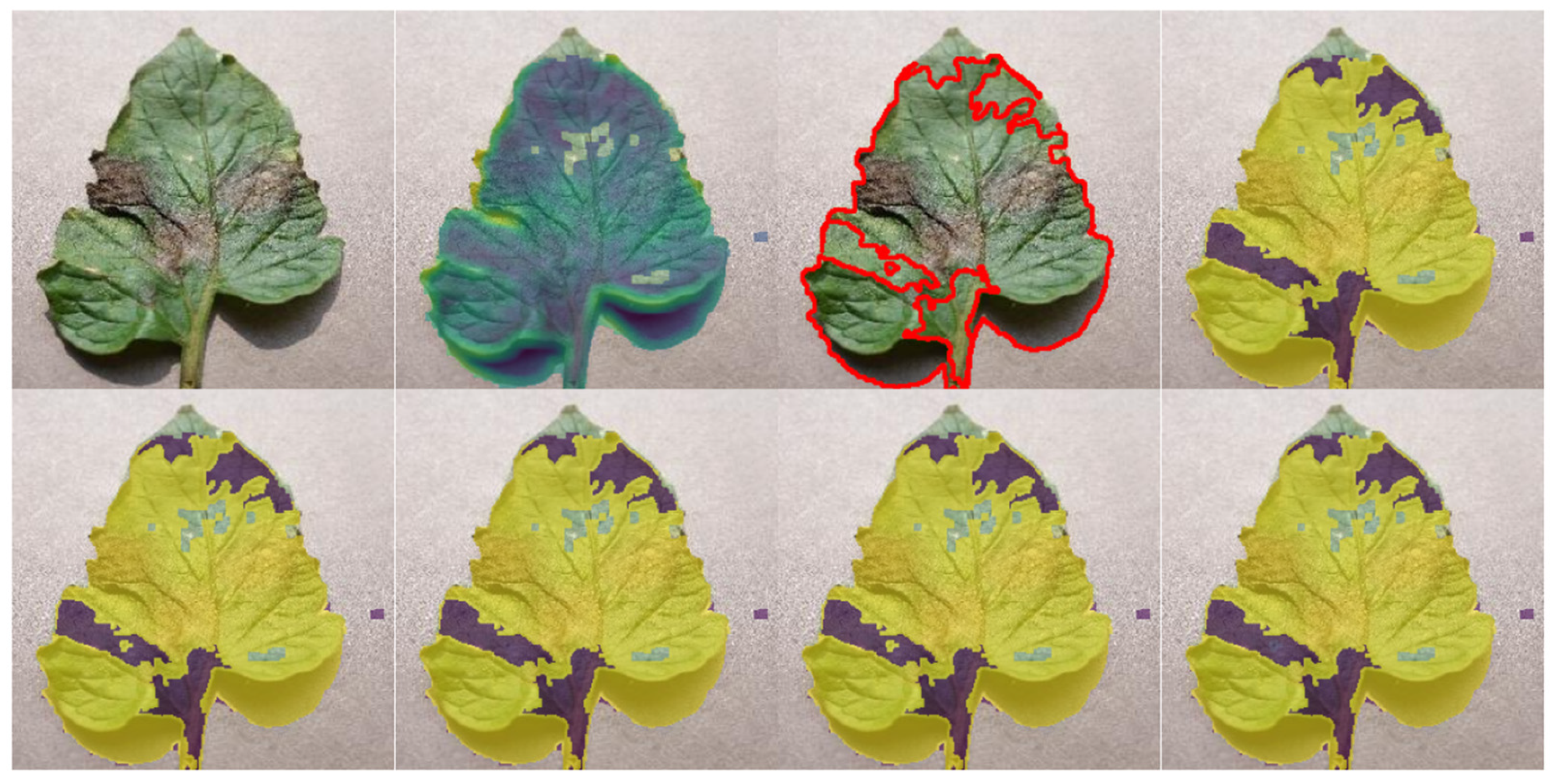
Figure 3. Geometric texture descriptor.
Agriengineering 08 00098 g003
Figure 4. Boosting loss functions.
Agriengineering 08 00098 g004
Figure 5. Input image. (a) Healthy leaf, (b) 1st stage, (c) 2nd stage, (d) 3rd stage, and (e) 4th stage.
Agriengineering 08 00098 g005
Figure 6. Visualization of extracted texture–geometric descriptors, (a) Otsu’s method, (b) contrast, (c) num_contours, (d) mean_contour_area, (e) std_contour_area, (f) mean_contour_perimeter, (g) std_contour_perimeter, and (h) mean_area_to_perimeter_ratio.
Agriengineering 08 00098 g006
Figure 7. Visualizing GridSearchCV results for XGBoost hyperparameter tuning.
Agriengineering 08 00098 g007
Figure 8. Confusion matrix illustrating the classification performance of the proposed model.
Agriengineering 08 00098 g008
Table 1. Fragments of the training sample.
Objects x 1 x 2 x 3 x 4 x 5 x 6 x 7 Classes
S 1 37.3658824750491474541.6731543624161061096.15880956610438.33057982729585383.116454927420720.0698983762629732 K 1
S 1 49.9277151192824575799.966858.5628522599445.5727153412501309.371472891123230.3879013626354471 K 1
S 2 44.800203163762916107031.04252336448598921.822654510797611.55998361277803133.915577194182050.05231692861451514 K 2
S 2 35.32940780603492124226.27012882447665897.82605537036846.992370426366871103.710632064341670.032662478234222254 K 2
S 3 36.33191702294344129125.538729666924866884.19312649705066.70747675893844291.272370811404510.03187086575374872 K 3
S 3 51.03817701483962683037.8596385542168651050.18603079386310.271922461239688145.634918613609530.0476645162238748 K 3
S 4 51.8068492649323750761.188362919132151344.055329339576211.741234552460545125.641608585195030.058907243655364615 K 4
S 4 38.43759350132606110728.365853658536587907.8612297551676.85833759111871473.441080533268750.04048500480098933 K 4
S 5 39.368361543602774124025.12983870967742848.38923830643186.50812600322308176.177331564441320.038053655871191874 K 5
S m x n x n x n x n x n x n x n K l
Table 2. Fragment of the training sample after normalization.
Objects x 1 x 2 x 3 x 4 x 5 x 6 x 7 Classes
S 1 0.520.0020.0190.0220.2140.0020.794 K 1
S 1 0.3190.0050.0420.0460.3260.0040.754 K 1
S 2 0.2670.0060.0490.0320.1610.0150.701 K 2
S 2 0.2460.0070.0520.0360.1640.0160.703 K 2
S 3 0.5760.0020.0190.0220.2180.0010.861 K 3
S 3 0.3490.0050.0370.0380.2030.0060.777 K 3
S 4 0.0750.0460.2310.0910.4410.0210.91 K 4
S 4 0.750.0010.0120.0180.1260.0020.943 K 4
S 5 0.8090.0160.0840.1040.5370.0090.5 K 5
S m x n x n x n x n x n x n x n K l
Table 3. Model evaluation (metric).
PrecisionRecallF1-ScoreSupport
00.970.970.97321
10.910.930.92120
20.950.850.90142
30.910.950.93258
40.920.920.92208
Accuracy 0.931049
Macro avg0.930.920.931049
Weighted avg0.930.930.931049
Table 4. Comparison of the proposed XGBoost method with baseline models.
MethodDataset/SplitAccuracyMacro-F1Inference Time/FramePeak RAM
XGBoost (proposed)Own dataset (5-fold cross-validation, 80/20 split)0.930.93≈35 мc≈120 MB
SVM (RBF)Own dataset (5-fold cross-validation, 80/20 split)0.880.87≈70 мc≈210 MB
Random ForestOwn dataset (5-fold cross-validation, 80/20 split)0.900.89≈55 мc≈190 MB
k-NNOwn dataset (5-fold cross-validation, 80/20 split)0.860.85≈90 мc≈250 MB
Logistic RegressionOwn dataset (5-fold cross-validation, 80/20 split)0.840.83≈30 мc≈110 MB
CNN block (control comparison)Own dataset (5-fold cross-validation, 80/20 split)0.950.94≈120 мc (GPU)≈600 MB
Table 5. Functional architecture of the proposed XGBoost-based tomato leaf disease recognition system.
Stage No.ModuleOperation/DescriptionInput/OutputParameters/ToolsNotes
1Data InputImport RGB tomato leaf images from datasetRGB image (1024 × 1024 px)OpenCV cv2.resize(), cv2.cvtColor()Raw image captured under natural light
2PreprocessingResize → convert to grayscale → normalizationGrayscale image [0–1]OpenCV cv2.resize(), cv2.cvtColor()Reduces computational cost, standardizes scale
3SegmentationApply global Otsu thresholding to isolate leaf areaBinary maskcv2.threshold(…, cv2.THRESH_OTSU)Separates leaf from the background
4Morphological FilteringMorphological opening + closingClean binary maskStructuring elements 3 × 3, 5 × 5Removes noise and small holes
5Contour DetectionApply Canny edge detector + dilationEdge map/contour setCanny (3 × 3 kernel)Extracts lesion boundaries
6Feature ExtractionCompute 7 texture–geometric descriptors: contrast, num_contours, mean/std contour area, mean/std contour perimeter, mean area/perimeter ratio, fractal dimensionFeature vector (7D)Custom Python feature script (Python 3.13)Represents leaf texture and lesion geometry
7Feature NormalizationNormalize features using MinMaxScaler or Z-scoreNormalized vectorScikit-learn MinMaxScalerEnsures comparable feature scales
8Classification (XGBoost)Train XGBoost model with K-fold cross-validation and GridSearchCVPredicted disease class (0–4)≈150 trees, learning rate = 0.2Tuned for optimal accuracy and F1-score
9Evaluation and VisualizationGenerate a confusion matrix, accuracy, and F1-score, and overlay the segmentation maskQuantitative + visual outputsmatplotlib, seabornVisual analysis of correctly and incorrectly classified leaves
Disclaimer/Publisher’s Note: The statements, opinions and data contained in all publications are solely those of the individual author(s) and contributor(s) and not of MDPI and/or the editor(s). MDPI and/or the editor(s) disclaim responsibility for any injury to people or property resulting from any ideas, methods, instructions or products referred to in the content.