Abstract
As precision agriculture places higher demands on real-time field weed detection and recognition accuracy, this paper proposes a multi-scale information-enhanced weed detection algorithm, MIE-YOLO (Multi-scale Information Enhanced), for precision agriculture. Based on the popular YOLO12 (You Only Look Once 12) model, MIE-YOLO combines edge-aware multi-scale fusion with additive gated blocks and two-stage self-distillation to boost small-object and boundary detection while staying lightweight. First, the MS-EIS (Multi-Scale-Edge Information Select) architecture is designed to effectively aggregate and select edge and texture information at different scales to enhance fine-grained feature representation. Next, the Add-CGLU (Additive-Convolutional Gated Linear Unit) pyramid network is proposed, which enhances the representational power and information transfer efficiency of multi-scale features through additive fusion and gating mechanisms. Finally, the DEC (Detail-Enhanced Convolution) detection head is introduced to enhance detail and refine the localization of small objects and fuzzy boundaries. To further improve the model’s detection accuracy and generalization performance, the DS (Double Self-Knowledge Distillation) strategy is defined to perform double self-knowledge distillation within the entire network. Experimental results on the custom Weed dataset, which contains 9257 images of eight weed categories, show that MIE-YOLO improves the F1 score by 1.9% and the mAP by 2.0%. Furthermore, it reduces computational parameters by 29.9%, FLOPs by 6.9%, and model size by 17.0%, achieving a runtime speed of 66.2 FPS. MIE-YOLO improves weed detection performance while maintaining a certain level of inference efficiency, providing an effective technical path and engineering implementation reference for intelligent field inspection and precise weed control in precision agriculture. The source code is available on GitHub.
1. Introduction
With global population growth and the acceleration of agricultural modernization, precision agriculture technology is gaining widespread attention as an important means of increasing crop yields, reducing chemical inputs, and achieving sustainable management. In field management, weeds have complex spatial distribution, diverse species, and similar morphology to crops. Traditional manual inspection and general image processing methods are no longer able to meet the requirements of high-precision, low-cost, and real-time detection [1]. Therefore, deep learning-based visual inspection technology, especially lightweight one-stage object detectors with real-time reasoning capabilities, has become a key technical path to achieve intelligent field inspection and precision weed control [2].
In recent years, deep learning-based target detection methods have received widespread attention in the field of precision agriculture. By constructing a neural network model, the positioning and classification of targets in images can be achieved [3]. According to the different detection processes, the mainstream methods can be divided into two categories: two-stage algorithms and one-stage algorithms [4]. Two-stage algorithms include RCNN [5], SPPNet [6], Fast RCNN [7], Faster RCNN [8] and FPN (Feature Pyramid Networks) [9]. One-stage algorithms include YOLO (You Only Look Once) [10], SSD (Single Shot MultiBox Detector) [11], RetinaNet [12], CornerNet [13], CenterNet [14] and DETR (Detection Transformer) [15]. The two-stage algorithm first generates candidate regions and then performs fine classification and regression on each region, achieving high accuracy and flexible scalability. The one-stage algorithm completes target classification and regression simultaneously in a single forward pass, providing excellent real-time performance and ease of deployment.
As a representative method in the field of one-stage target detection, the YOLO series of algorithms has been widely used in many fields due to its excellent detection speed and accuracy. After the classic YOLOv5, YOLOv8 and YOLOv9 [16] algorithms, YOLOv10 [17], YOLO11 [18], YOLO12 [19] and YOLO13 [20] algorithms have been released one after another, and the detection performance has been further improved.
However, for precision agriculture, the standard YOLO model often performs poorly in multi-scale small object detection. Small weeds occupy few pixels so downsampling loses key texture and shape cues, causing missed or merged detections. Scale variation, occlusion, and dense vegetation further hurt localization and classification, and common design choices such as anchors and non-maximum suppression can suppress true small-object predictions. Field images also introduce domain shifts from lighting, motion blur, and different sensors, and real-time constraints on embedded hardware prevent simply enlarging the network. Therefore, this paper proposes a multi-scale information enhancement weed detection algorithm that is committed to balancing running speed and detection accuracy. The contributions of this paper are summarized as follows:
(1) A new MS-EIS (Multi Scale-Edge Information Select) architecture was designed to address the difficulty of detecting small objects and targets in complex backgrounds by selectively aggregating edge and texture information across multiple scales, thereby enhancing fine-grained feature representation.
(2) A new Add-CGLU (Additive-Convolutional Gated Linear Unit) pyramid network was proposed to handle multi-scale variation by improving the representation capability and information transmission efficiency of features through additive fusion and gating mechanisms, helping the network better capture small objects in complex scenes.
(3) A new DEC (Detail-Enhanced Convolution) detection head was developed to mitigate the challenge of imprecise localization in small objects and blurred boundaries by strengthening detail features and refining spatial positioning, improving detection in cluttered or challenging backgrounds.
(4) A new DS (Double Self-Knowledge Distillation) strategy was defined to overcome generalization degradation under complex scenes by performing dual self-distillation across the whole network, further improving detection accuracy and robustness, ensuring reliable performance even with small or difficult-to-distinguish targets.
2. Related Work
Advances in computer vision have driven the application of object detection algorithms in precision agriculture, including targeted weed control, pest and disease monitoring, and fruit crop counting. Deep learning-based object detection algorithms have gradually replaced traditional manual feature extraction methods and become the mainstream choice for field weed detection. Many studies, mostly based on deep learning algorithms, aim to improve the accuracy and real-time performance of dense weed detection in fields by improving the backbone network, incorporating attention modules and multi-scale feature fusion, expanding the receptive field and contextual information, and optimizing lightweight post-processing.
Some researchers have improved the accuracy and precision of the classic YOLOv5 algorithm, pioneering the module fusion approach. Deng et al. [21] proposed an accurate and effective weed detection model HAD-YOLO based on the improved YOLOv5 network. The algorithm uses HGNetv2 as its backbone network, introduces the SSFF (Scale Sequence Feature Fusion) module with attention mechanism to improve the feature extraction ability of the model. Wang et al. [22] proposed an advanced weed detector based on enhanced YOLOv5, which combines CBAM (Convolutional Block Attention Module), FasterNet feature extraction network and loss function to optimize the network structure and training strategy. Tao and Wei [23] proposed a rapeseed field weed detection network STBNA-YOLOv5 based on the improved YOLOv5, which enhances the feature extraction ability through the Swin Transformer, uses the BiFPN to fuse the NAM (Normalization-based Attention Module) to utilize feature information. Zhang et al. [24] proposed a weed detection method CCCS-YOLO based on lightweight and contextual information fusion, which promotes the fusion of contextual information by integrating Faster Block, context aggregation module and CARAF (Content-Aware ReAssembly of Feature).
Some researchers have also made lightweight improvements based on the popular YOLOv8 algorithm, achieving some progress in real-time performance optimization. Hu et al. [25] proposed a lightweight and high-precision precision agriculture cotton weed recognition model CW-YOLO based on YOLOv8. The network introduced a dual-branch structure that combines visual transformers and convolutional neural networks, and proposed an RFE (Receptive Field Enhancement) module to reduce computational complexity and the number of parameters. Chen et al. [26] proposed a rice field weed detection algorithm GE-YOLO based on YOLOv8, which introduced a distribution network with feature aggregation and an EMA (Efficient Multi-scale Attention) mechanism to enhance the network’s ability to fuse multi-scale features and detect weeds of different sizes. Zheng et al. [27] proposed a cotton field weed recognition algorithm YOLOv8-DMAS based on optimized YOLOv8, which improved the accuracy of dense weed detection through the DWR (Dilation-Wise Residual) module, and the ASFF (Adaptively Spatial Feature Fusion) mechanism. Shuai et al. [28] proposed a real-time weed detection model YOLO-SW for soybean fields based on the improved YOLOv8, introducing the Swin Transformer backbone network to achieve efficient global context capture.
In addition, some researchers have made recent progress in designing network architectures based on CNNs, which have improved the efficiency of target detection in the field of precision agriculture. Umar et al. [29] proposed a deep learning-based lavender classification method to enhance cultivation and essential oil quality management. The model was fine-tuned through transfer learning, learning rate adjustment, and batch optimization. Additional layers were added to the baseline model to improve classification performance and reduce training time. Gulzar [30] conducted a comparative study on papaya leaf disease classification based on pre-trained deep learning models, evaluating four pre-trained convolutional neural networks. He also proposed an AI-driven early detection and classification method for papaya leaf diseases, PapNet [31], which utilizes advanced architectural features, including global average pooling, dense layers, and strategic use of batch normalization and dropout, demonstrating superior performance in distinguishing various papaya leaf conditions. Han et al. [32] proposed a precision agriculture segmentation technique for coconut diseases based on enhanced remote sensing images. They developed a robust disease segmentation model using a pre-trained CNN, which can improve disease management in coconut cultivation.
Although YOLO-based weed detection has advanced rapidly, existing methods still face important limitations. YOLOv5-based models, such as HAD-YOLO and STBNA-YOLOv5, improve feature extraction with attention modules or transformers, but often increase computational cost and struggle in resource-limited field scenarios. YOLOv8-based models, including CW-YOLO and GE-YOLO, achieve lighter designs and multi-scale fusion, yet they still have difficulty detecting small, dense, or overlapping weeds in complex backgrounds. In contrast, the proposed method introduces a multi-scale, detail-enhanced, and distillation-guided framework that aggregates edge and texture information, improves multi-scale feature fusion, and leverages dual self-knowledge distillation. This approach enhances detection of small and dense weeds, increases robustness in cluttered environments, and maintains a balance between accuracy and real-time performance that previous YOLO-based methods have not fully achieved.
3. Methodology
3.1. Overall Network Structure
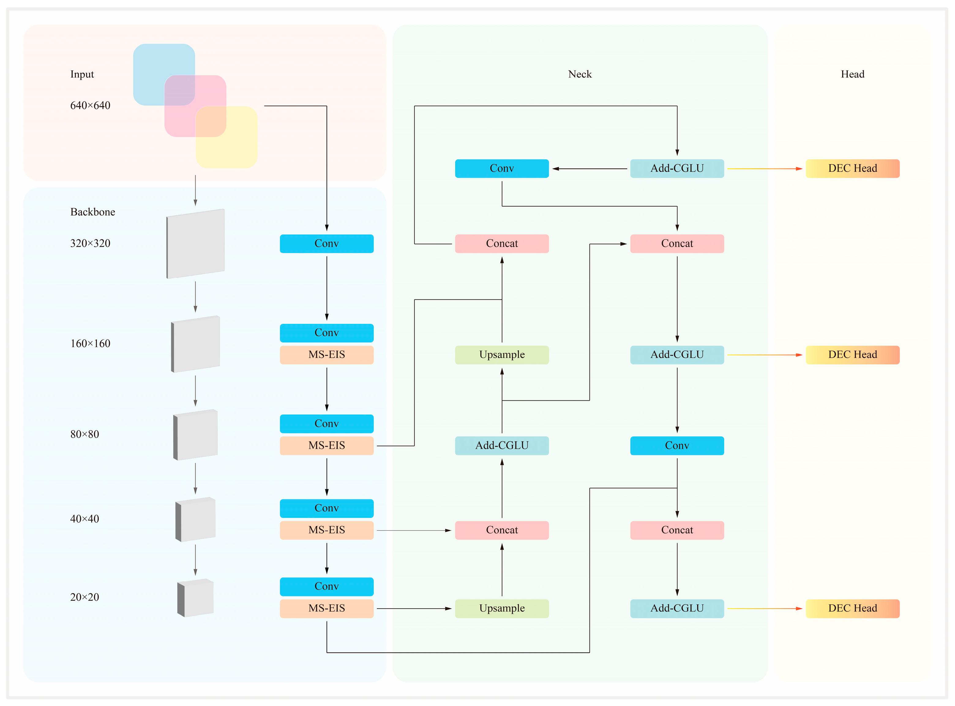
Based on the YOLO12-N model, this paper independently designed the MS-EIS (Multi-Scale-Edge Information Select) architecture, the Add-CGLU (Additive-Convolutional Gated Linear Unit) pyramid network, and the DEC (Detail-Enhanced Convolution) detection head. Finally, the DS (Double Self-Knowledge Distillation) strategy was combined to perform knowledge distillation on the overall structure, resulting in the proposed MIE-YOLO. Its overall network structure is shown in Figure 1.
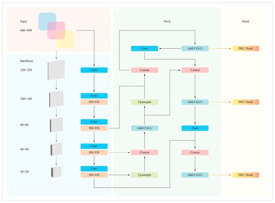
Figure 1.
MIE-YOLO overall network structure.
3.2. Multi-Scale-Edge Information Select Architecture
The original YOLO12 framework consists of three basic components: Backbone, Neck, and Head, each implementing a different function. The Backbone of YOLO12 is the core component responsible for feature extraction. Through multi-layer convolution operations and a modular structure, it converts the input image layer by layer into multi-scale feature maps for subsequent detection tasks. This sub-module stack includes the C3k2 module and the A2C2f (Area Attention) module, which extracts multi-scale features containing rich semantic information.
Compared to previous versions, YOLO12 introduced the C3k2 module and the A2C2f module, replacing the C2f module used in previous generations. The C3k2 module uses two small kernel convolutions instead of one large kernel, aiming to preserve both global and local information of features. The A2C2f module maintains a large receptive field, aiming to reduce the computational complexity of attention in a simple way and thus increase speed. However, these modules still contain a large number of bottleneck structures, which can lead to vanishing gradients and feature redundancy, weakening the global receptive field coverage.
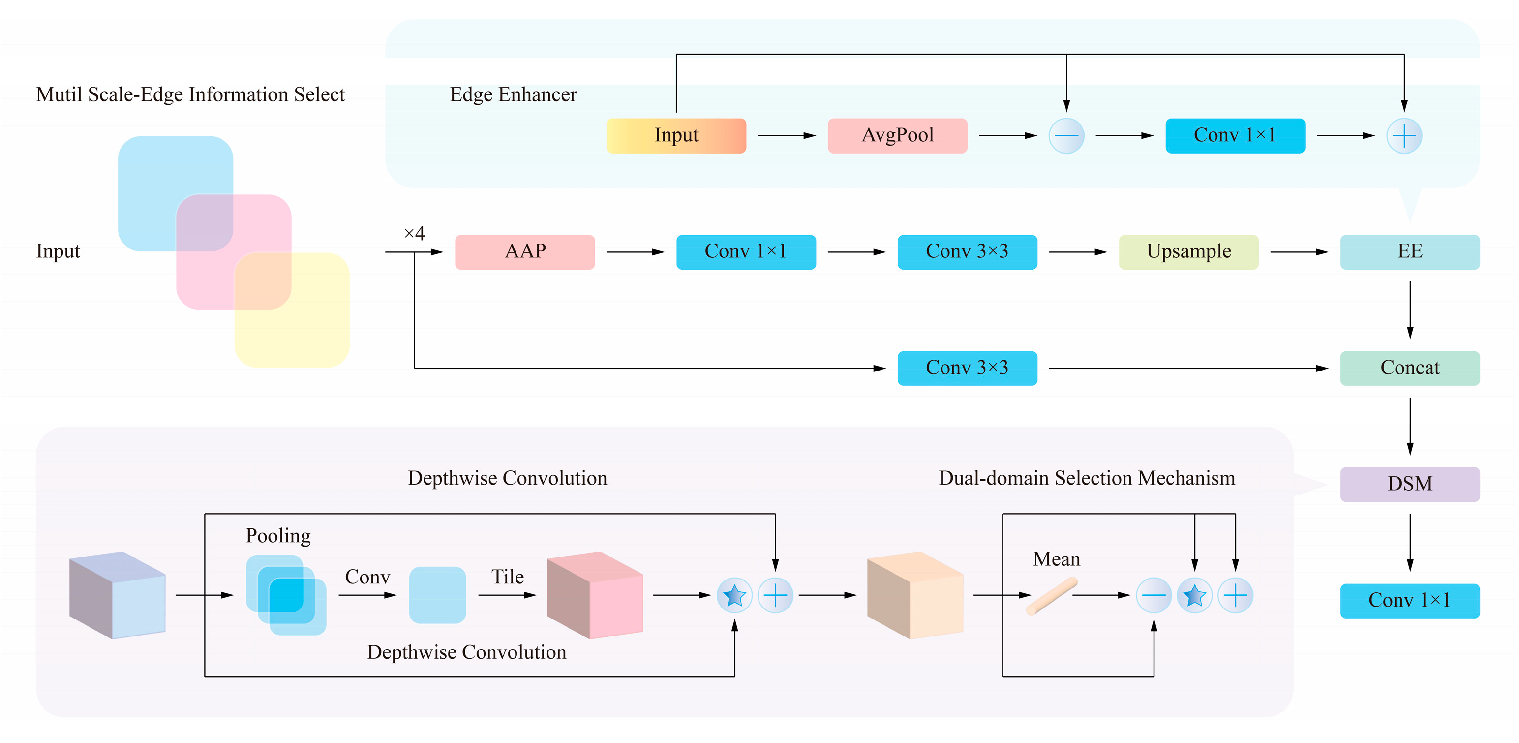
To address these challenges, the C3k2 and A2C2f modules in the Backbone architecture were redesigned. Specifically, a new EE (Edge Enhancer) module was developed, and the DSM (Dual-domain Selection Mechanism) proposed by Cui et al. [33] was incorporated to propose a new MS-EIS (Multi-Scale-Edge Information Select) architecture to replace the Bottleneck in the C3k2 and A2C2f modules. The structure of the MS-EIS architecture is shown in Figure 2.
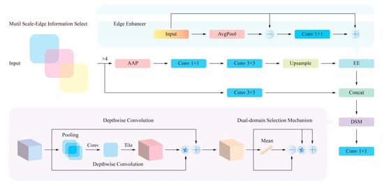
Figure 2.
Multi-Scale-Edge Information Select architecture.
MS-EIS replaces the simple bottleneck used in YOLO12’s backbone with an integrated module that goes beyond the original DSM by combining principled multi-scale pooling with learnable scale weights, an explicit edge enhancement path based on Laplacian filtering balanced by Gaussian denoising, and an efficient depthwise separable convolution preprocessing stage, all fused by a targeted attention scheme. Compared to simply referencing the original DSM, MS-EIS is more prescriptive and reproducible because it specifies concrete operators and hyperparameters, it introduces an explicit signal-processing style edge path that DSM lacks, and it trades a small amount of added structure for substantial improvements in boundary and small-object sensitivity while maintaining a low computational profile.
Edge information is a consistent and discriminative cue that separates weeds from crops, especially in early growth stages when color and texture signals are weak and plant instances are small, so leaf contours, margins, and vein-defined edges become the most reliable features for distinguishing species. Edges encode shape and boundary geometry that are less sensitive to illumination shifts and color similarity, they provide strong localization anchors for tiny and partially occluded plants, and they help disambiguate overlapping instances by revealing separate object contours. MS-EIS treats edge cues as a first-class signal rather than an incidental feature, so it explicitly extracts high frequency content with a Laplacian path and then stabilizes that signal with Gaussian denoising, while multi scale pooling and learnable scale weights allow the module to emphasize the most relevant edge scales for a given scene or growth stage. This differs from common attention modules such as CBAM which reweight channels and spatial locations on the existing feature maps but do not create a dedicated, signal-processing style edge channel, and it differs from simple Sobel fusion which injects a fixed single scale gradient that amplifies noise and cannot adapt to scale, blur, or imaging conditions. By combining principled filtering, adaptive scale weighting, and efficient depthwise separable preprocessing, MS-EIS amplifies true boundary cues while suppressing noise and keeping computation low, yielding clearer boundaries, better small object localization, and greater robustness in cluttered agricultural scenes than either generic attention or naive fixed edge fusion.
MS-EIS (Multi-Scale-Edge Information Select) is a deep learning feature enhancement module optimized for object detection, segmentation, and feature extraction tasks. Its primary goal is to improve the model’s object detection capabilities in complex scenes through multi-scale feature fusion and edge information enhancement. This architecture combines multi-scale feature extraction, edge information enhancement, deep convolution operations, and a dual region-focused attention mechanism to optimize the effectiveness and robustness of feature extraction. The key concept in the MS-EIS architecture is to utilize multi-scale average pooling and adaptive convolution to extract feature information at different levels, combined with an edge enhancement module for feature comparison and supplementation, and ultimately achieve efficient feature fusion through a dual region selection mechanism. This process enables MS-EIS to simultaneously capture local details and global contextual information, improving detection accuracy while reducing computational costs.
Specifically, four parallel AAP (Adaptive Average Pooling) modules are first used to perform multi-scale adaptive average pooling to extract feature information at different scales. This is then combined with convolution operations to obtain rich semantic information. The core idea is to utilize pooling operations at different scales to capture global and local information with different receptive fields. Assuming an input feature X, the input feature map can be represented as follows:
where the real number space ℝ is used to describe the range of the feature map, and i is mainly used to index the feature extraction process at different scales, specifically indicating the feature processing step at the i-th scale. H and W are the height and width of the feature map, respectively, and C is the number of channels of the input and output features. Multi-scale adaptive pooling is combined with the corresponding convolution operation on the input feature map to construct a feature pyramid:
where Pooling represents an adaptive pooling operation of scale i. Through pooling operations of different scales, different resolution versions of the feature map are extracted, so that the network can focus on large targets, medium targets and small targets at the same time. Conv represents the convolution operation of the i-th level. The first convolution with a spatial dimension of 1 is used to reduce the dimension and enhance the information interaction between channels, providing more effective input for subsequent convolution operations. The second convolution with a spatial dimension of 3 further extracts local features and improves the detection ability of edges and small targets. σ represents normalization and nonlinear activation operations, which transforms the features through the corresponding activation functions to make them more expressive. Upsample represents the upsampling operation, which is used to restore the size of the input features.
Pooling at different scales preserves multi-level features, improving adaptability to small objects and complex backgrounds. Multi-scale pooling also extracts local information of varying sizes, helping to capture the multi-level features of an image. Softmax is then used to weight features at different scales, resulting in smoother fusion without relying on manually configured hyperparameters. Finally, the multi-scale fused feature, ƑMS, is calculated as follows:
where ƑMS represents the final fused multi-scale features, and α is the normalized feature weighting coefficient used to weight feature maps at different scales. β is a learnable parameter representing the original weight of the feature weighting coefficient. βi is a scalar value obtained through neural network training and determines the size of αi. j is an index variable used to indicate the summation range of feature weights calculated at all scales. The softmax mechanism adaptively adjusts the weights of features at different scales, allowing the model to automatically select the most important scale features. Furthermore, the introduction of learnable parameters allows features of different scales to contribute differently to the final fusion, improving the flexibility of feature extraction. The final fused multi-scale features take into account the feature representation of both large and small objects.
We initialize each β to zero so the softmax produces equal weights across scales at the start, providing a neutral baseline. Each β is then learned as a scalar parameter by the usual backpropagation process but with conservative optimization settings, for example a reduced learning rate or a dedicated learning-rate multiplier and minimal or no weight decay, to avoid abrupt or biased shifts in the fusion distribution. If training is unstable, simple stabilizers can be used such as freezing β for a short warmup period, applying gradient clipping, or adding a softmax temperature greater than one to smooth the resulting weights. During training we monitor the resulting α values and include an ablation that compares fixed versus learnable β to verify the benefit of learned scale weighting.
The EE (Edge Enhancer) module is a key component in the MS-EIS architecture. Its primary function is to address the traditional Bottleneck architecture’s inability to extract edge information and improve the ability to identify target edge contours. The core concept of the EE module is to extract edge information using Gaussian filtering and the Laplacian operator, and then fuse feature maps through convolution. In this step, edge information is first calculated:
where Edge represents the extracted edge information, and the partial differential equation represents the Laplacian operation. Gσ represents the standard Gaussian kernel, which displays the Gaussian filtering results and is mainly used for denoising. λ is a balance parameter that controls the weighting of Gaussian filtering and gradient enhancement. Next, a standard convolutional layer is used to perform a nonlinear transformation on the edge features and then add them to the original features to obtain the edge features:
where ƑEE represents the final enhanced edge feature, and σ represents the nonlinear transformation. The EE module improves the model’s perception of boundary information through edge enhancement, facilitating accurate target localization. Furthermore, it combines Gaussian filtering and the Laplacian operator to enhance edges while minimizing noise interference.
Overall, the EE module extracts edge information, enhancing the network’s sensitivity to edges. This is crucial for visual tasks such as object detection and semantic segmentation. The Concat module then interpolates features extracted at different scales to align them to the same scale and concatenates them. Finally, a standard convolutional layer fuses these features into a unified feature representation, improving the model’s perception of multi-scale features.
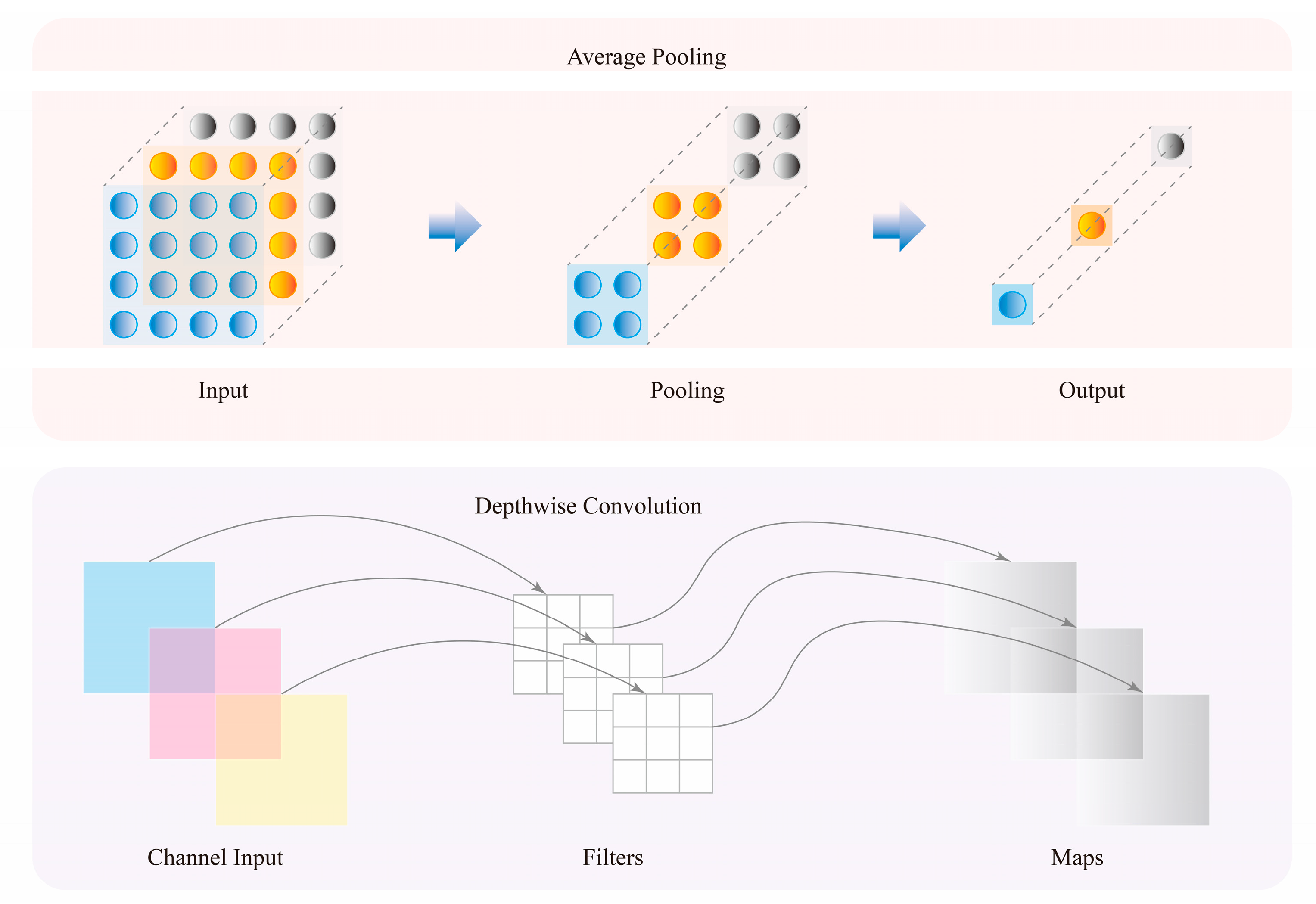
Finally, all features are fed into the DSM (Dual-domain Selection Mechanism). This attention mechanism aims to efficiently select key features highly relevant to the target task from multi-scale-edge information. By focusing on more important areas in the image, such as complex edges and high-frequency signals, this mechanism adaptively selects features with higher task relevance from the multi-scale features, significantly improving feature selection accuracy and overall model performance. Figure 3 shows the detailed structure of each submodule in the DSM.
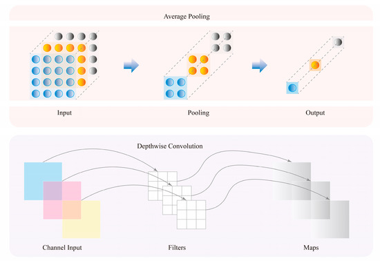
Figure 3.
Dual-domain Selection Mechanism submodule.
The DSM module addresses feature redundancy by selecting the most important features in both the channel and spatial domains to improve detection accuracy. First, two depthwise separable convolutions are used to reduce computational complexity while enhancing feature representation. Depthwise separable convolution decomposes the standard convolution into DC (Depthwise Convolution) and PC (Pointwise Convolution), resulting in the following output feature maps:
where C is the number of input and output feature channels, and k is the convolution kernel size. Yd represents the intermediate feature map after depthwise convolution, and Wd is the convolution kernel for depthwise convolution. Yp represents the output feature map after pointwise convolution, and Wp is the weight matrix for pointwise convolution. ReLU represents the activation function used for nonlinear transformations, ƑDW is the final activated depthwise separable convolution output, and O represents computational complexity. The left side represents standard convolution, and the right side represents depthwise separable convolution. Compared to standard convolution, depthwise separable convolution reduces computational complexity by approximately k2 times. When k is 3, the computational complexity is reduced by approximately 9 times.
The dual region information selection mechanism enhances the information expression capabilities of the channel domain and the spatial domain. That is, the DSM module combines the CA (Channel Attention) and SA (Spatial Attention) mechanisms, allowing the model to focus on the salient features of the target while ignoring unimportant information. First, the feature importance weight is calculated in the channel dimension:
where Mc represents the channel attention weight matrix, which evaluates the importance of different channels. Wc represents the learnable parameter matrix used for channel weighting, which adjusts the contribution of different channels. Pooling represents the GAP (Global Average Pooling) operation, which is used to obtain global information for each channel. i and j represent the pixel values of the feature map, respectively.
Compared to the traditional attention mechanism, channel attention only involves the channel dimension and does not consider spatial information, so the computational cost is lower. Afterwards, the feature response is calculated in the spatial dimension:
where Ms represents the spatial attention weight matrix, which indicates the importance of different spatial locations. Ws is the learnable parameter matrix used for spatial weighting, which adjusts the contribution of different spatial regions. Large kernel convolution is used to extract spatial features over a wide range, enhancing the integrity and shape perception of the object.
Compared to channel attention, spatial attention focuses directly on the spatial distribution of feature maps, highlighting important target areas while suppressing irrelevant areas. By learning weights for different spatial locations, the model can more accurately locate the target and reduce background interference. Ultimately, the output of the DSM module is as follows:
where ƑDSM represents the final output feature of the dual region selection mechanism, and element-wise multiplication is used to weight different feature maps. The deeply weighted features are influenced by both channel and spatial attention, ensuring that the final fused features are optimally selected in both the channel and spatial dimensions. Because the attention mechanism suppresses irrelevant features, the feature maps output by the DSM module contain more compact information, thereby improving computational efficiency. For detection tasks, the edge and semantic features of key objects are significantly enhanced, which helps improve small object detection capabilities.
Finally, the features output by the DSM module are transformed and fused through a standard convolutional layer to obtain the final output of the MS-EIS architecture:
where Output represents the feature output of the MS-EIS architecture. The standard convolutional layer serves as the final feature mapping unit, which optimizes cross-channel information fusion, enables multi-scale feature extraction and dual region information selection to work together, and improves the accuracy and robustness of target detection.
Overall, MS-EIS has efficient multi-scale information integration capabilities. Its core components include adaptive average pooling, edge enhancement module, and dual region information selection mechanism, which synergistically improve target detection performance. First, MS-EIS uses AAP combined with convolution operations to enhance the perception of targets of different scales and improve the scale adaptability of detection. Secondly, the EE module optimizes the target contour features through edge information enhancement, making the target more prominent in complex backgrounds, thereby improving the robustness of target detection. Meanwhile, DSM combines channel attention and spatial attention to filter key features in the channel domain and spatial domain, effectively reducing redundant information and further improving detection accuracy.
Furthermore, MS-EIS employs a lightweight pooling and attention-weighted mechanism for efficient information screening and fusion, ensuring high accuracy while also balancing computational efficiency, making it suitable for real-time tasks. Specifically for small target detection, spatial attention enhances target edge information, the EE module strengthens target contours, and multi-scale feature extraction further enhances the saliency and detection of small targets. Overall, the MS-EIS architecture achieves efficient and accurate target detection through the coordinated optimization of multi-scale feature extraction, edge information enhancement, and dual region information selection.
3.3. Additive-Convolutional Gated Linear Unit Pyramid Network
The Neck portion of the original YOLO12 is located between the Backbone and the Head. Its main function is to fuse and enhance the multi-scale features extracted by the Backbone and pass them to the Head for prediction. The feature pyramid structure combines upsampling and cross-scale connections to achieve adaptive detection of multi-scale targets, while taking into account both global context and local details. Although the Neck simplifies computational complexity to a certain extent, the upsampling process may lead to loss of details or reduced positioning accuracy, especially in the detection of small targets or targets with blurred boundaries. At the same time, multi-scale feature splicing can easily introduce information redundancy, interfere with the expression of effective features, and increase the possibility of false detection or missed detection. In addition, deep features may cover the local details of shallow features, weakening the ability to capture small targets.
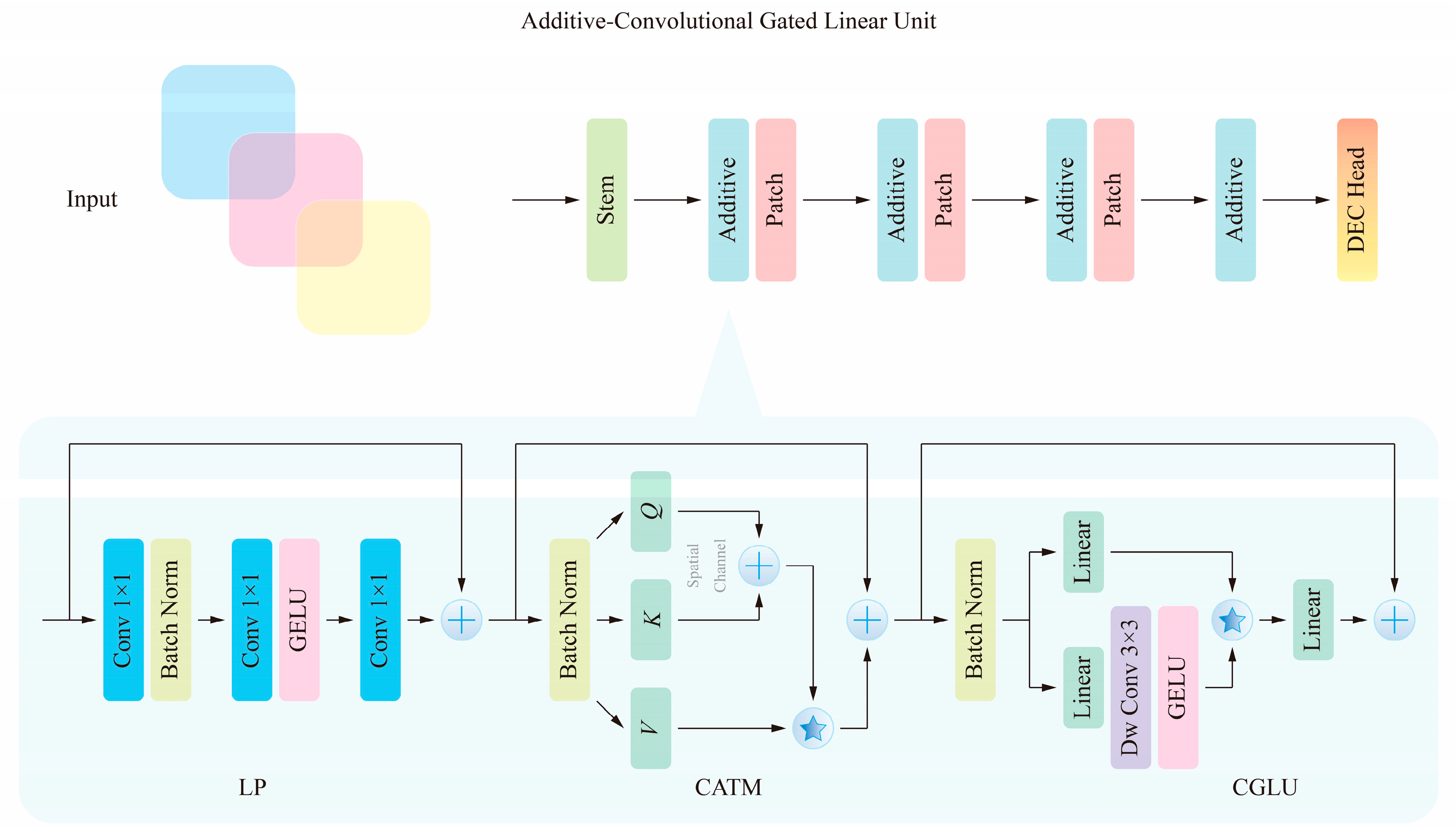
To ensure both real-time target detection and improved accuracy, a new Add-CGLU (Additive-Convolutional Gated Linear Unit) pyramid network was designed to optimize the Neck portion. This architecture draws inspiration from the CAS-ViT structure proposed by Zhang et al. [34], replacing the stacked Bottleneck with Additive Blocks. The new Add-CGLU pyramid network was designed by drawing on the Convolutional GLU (Gated Linear Unit) framework proposed by Shi [35]. The structure of the Add-CGLU pyramid network is shown in Figure 4.
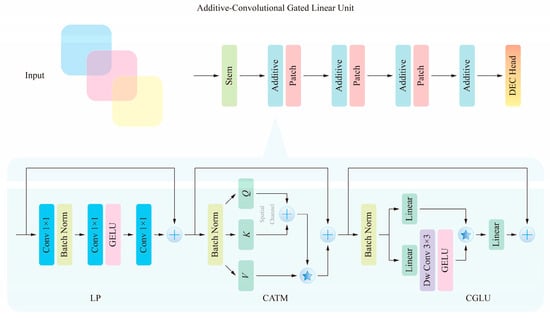
Figure 4.
Additive-Convolutional Gated Linear Unit pyramid network.
The Add-CGLU pyramid replaces stacked bottlenecks with Additive Blocks that combine three coordinated components: a Local Perception stage that preserves shallow spatial detail through standard convolutions, batch normalization and GELU; a Convolutional Additive Token Mixer that captures global context using an additive attention scheme to avoid the quadratic cost of conventional self-attention; and a Convolutional Gated Linear Unit that fuses depthwise convolution with a gating path for efficient feature filtering. Alternating Additive Blocks and patch segmentation give the neck a scalable multi scale fusion pattern while the Stem and pooled head keep integration simple. Compared with CAS-ViT and a plain GLU, this design is more convolution centric, more computationally efficient, and more prescriptive about operators and hyperparameters; it better preserves local detail while still capturing global context, reduces attention overhead, and is easier to reproduce and deploy for real time and small object detection.
Although gating mechanisms, such as the Gated Linear Unit, have been widely adopted in both Transformer and CNN architectures to modulate information flow, the combination of additive fusion and gating proposed in this manuscript represents a distinct structural innovation, rather than a simple application of existing components. In this design, the additive fusion integrates multiple feature streams in a complementary manner before the gating operation selectively filters and emphasizes informative patterns. This sequential coordination enables more precise feature modulation compared with conventional convolutional layers or standard residual blocks, which typically rely on linear summation or identity shortcuts without adaptive feature weighting. As a result, the network achieves higher computational efficiency, since additive fusion reduces redundant computations and mitigates the quadratic complexity associated with traditional self-attention, while the gating mechanism ensures that only salient features are propagated forward. Empirically, this synergy improves the representation of fine-grained local details and strengthens global context modeling, leading to better detection performance, particularly for small objects and real-time scenarios, without increasing the model’s parameter or inference overhead.
In the Add-CGLU pyramid network, the Stem module is located at the initial input stage and is responsible for converting the raw input into appropriate feature representations. Alternating Additive Block and Patch Segmentation modules divide the feature map into multiple small patches, while the classification detection head performs global pooling on the final features and outputs the classification results.
The Additive Block is the core module in the Add-CGLU architecture, comprising the LP (Local Perception) mechanism, CATM (Convolutional Additive Token Mixer), and CGLU (Convolutional Gated Linear Unit). The LP mechanism utilizes local integration to extract local spatial information from input features, overcoming the receptive field limitations of standard convolutional layers. Three standard convolutional layers, a Batch Normalization (BN) layer, and a nonlinear activation function, GELU (Gaussian Error Linear Units), are used to initially process the input features. Assuming x1 is the input feature, the process of extracting local spatial features using the LP mechanism can be represented as follows:
where Lp represents the local perception output, W is the weight function, BN represents batch normalization, and σ is the activation function.
After the input features are sensed and extracted by the LP mechanism, they are passed to the CATM component. First, a batch normalization layer and independent linear transformations are used to split the input information into three parts: Q, K, and V, corresponding to the query, key, and value matrices, respectively. This process is demonstrated using the input feature x2 mentioned above:
where Φ is the context mapping function, Ch represents the channel attention mechanism, Sp represents the spatial attention mechanism, and Ϻ is a Mirror function.
Overall, CATM aims to capture global contextual information through its core additive attention mechanism. Combined with the results of the Token Mixer, the architecture achieves optimized attention mechanisms at both the channel and spatial levels. This additive approach reduces computational overhead while maintaining the model’s ability to capture global dependencies, avoiding the quadratic complexity of matrix multiplication common in traditional self-attention mechanisms. The final output of CATM is as follows:
where Г is a linear transformation that integrates contextual information and includes necessary information interaction.
After the input features are enhanced by CATM, they are then processed by CGLU. CGLU combines depthwise convolution with a gating mechanism, enabling efficient feature filtering and spatial perception. A dual-branch structure consisting of a batch normalization layer, a standard convolutional layer, and a GELU activation function processes spatial information, enhancing the model’s ability to capture fine-grained features. The final output of the CGLU module is the element-wise multiplication of the results of the two branches:
where Wb1 and Wb2 correspond to the weights on each branch respectively. The CGLU implements the attention of the channel mixer with fewer computational parameters based on the channel attention mechanism of the nearest neighbor image feature fusion, thereby enhancing the robustness of the model.
3.4. Detail-Enhanced Convolution Detection Head
The head of the original YOLO12 is the final stage of the overall network structure, responsible for generating the final predictions for object detection and classification. Its core task is to process the feature maps passed from the neck, ultimately outputting bounding boxes and class labels for objects within the image. The head of YOLO12 refines features through further convolution operations and optimization modules, employing the C3k2 module to improve computational efficiency and feature representation. It also incorporates CBS (Convolution-Batch Norm-SiLU) to enhance the model’s stability and nonlinear representation capabilities.
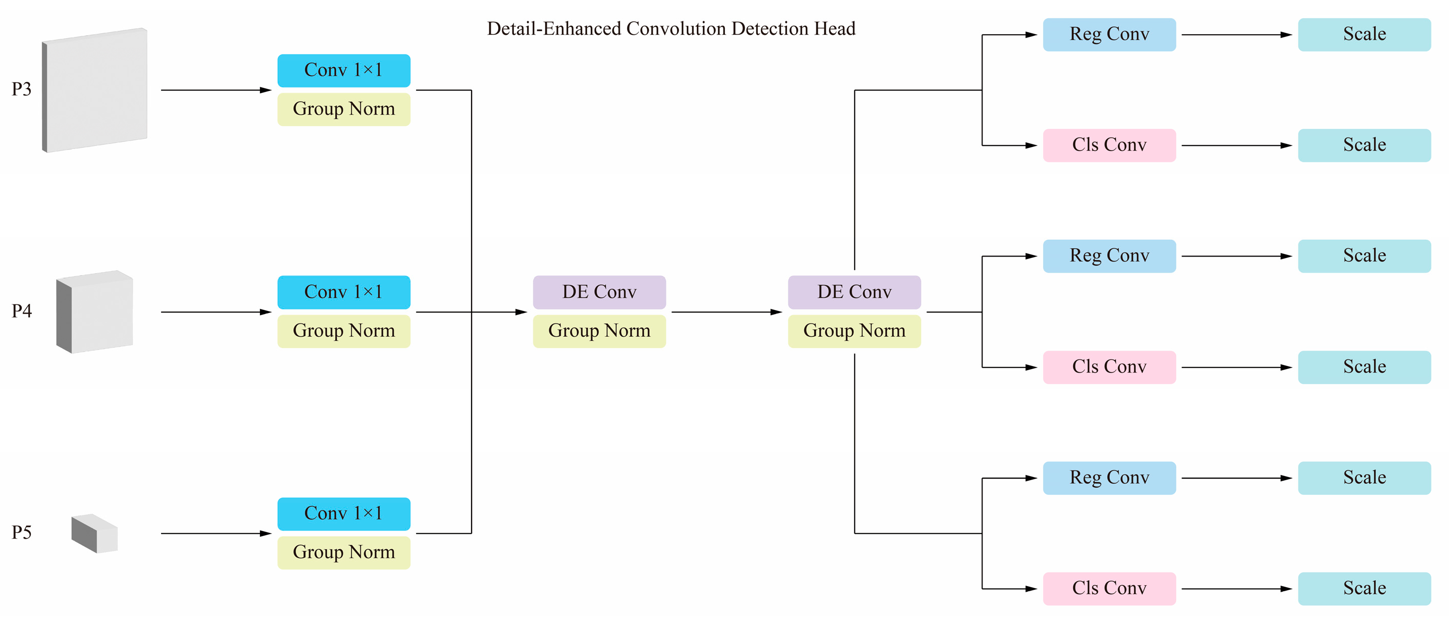
However, the original head also has some shortcomings. For example, it suffers from low localization accuracy for small objects, possibly due to loss of detail during upsampling or feature fusion, leading to inaccurate bounding box predictions. It is also susceptible to background interference in dense scenes, increasing the risk of false or missed detections. Furthermore, the computational overhead for high-resolution inputs is high, limiting its suitability for extreme real-time scenarios. To address these challenges, the original YOLO12 head framework has been re-optimized, and a new DEC (Detail-Enhanced Convolution) detection head has been proposed. The structure of the DEC detection head is shown in Figure 5.
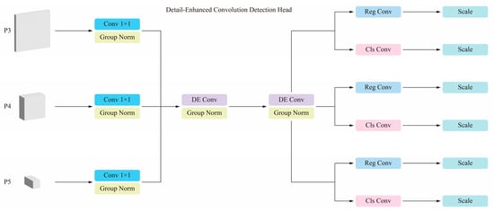
Figure 5.
Detail-Enhanced Convolution detection head.
The design goal of the DEC detection head is to improve fine-grained feature extraction capabilities through a shared feature enhancement module, aiming to optimize the detection efficiency of small objects in complex scenes. DE Conv (Detail-Enhanced Convolution) is the core component of the DEC detection head and was first proposed by Chen et al. [36] in DEA-Net (Detail-Enhanced Attention Network). By enhancing the input features, detail information is better preserved. During the feature fusion stage, DE Conv shares weight information at different feature scales, strengthening feature consistency and reducing computational cost.
Specifically, DE Conv combines the feature extraction capabilities of standard convolution with a detail-enhancing normalization strategy. It uses the GN (Group Normalization) layer to group and normalize features, reducing the impact of statistical noise during small-batch training and avoiding the instability of BN (Batch Normalization) during small-batch training. DE Conv first reduces the dimensionality of an input feature x3 and extracts spatial features:
where σ is the Sigmoid activation function, ensuring that the output range is between 0 and 1. Then use the content-guided attention mechanism to generate spatial weights for each position:
The weight distribution of the convolution kernel is then adjusted to better capture the details of the spatial features. The weight distribution of the features is then dynamically adjusted to adapt to local changes in the target. While improving the deep modeling capability, the grouping mechanism reduces computational redundancy and ensures the global representation capability of the features. The dynamic kernel generation process of DE Conv is as follows:
The end of the DEC detection head contains two submodules, Cls Conv (Classification Convolution) and Reg Conv (Regression Convolution), which are used for target category prediction and bounding box regression respectively. Cls Conv maps the feature map to the category space and uses the Sigmoid activation function to generate the category probability of each anchor, while Reg Conv outputs the regression parameters of each anchor bounding box. The parameters in Cls Conv are also shared. Whether it is a small, medium or large target, it is the same target for classification learning. The DEC detection head uses a separable loss function, including classification loss and regression loss, which can be expressed as follows:
where represents the classification and regression losses, and λ is the corresponding weight hyperparameter. Furthermore, the shared parameters in Reg Conv need to account for the impact of inconsistent object scales, thus scaling the features through the Scale layer. The Scale operation is also shared, allowing the regression output to be adjusted to accommodate objects of varying scales.
In the DEC detection head, the Detail-Enhanced Convolution module is further refined through the use of dilated convolutions and content-adaptive filter selection. Specifically, dilated convolutions expand the receptive field without increasing the number of parameters, enabling the network to capture broader contextual information around small objects while preserving fine-grained local features. Meanwhile, DE Conv dynamically adjusts its convolutional kernels based on the content-guided attention maps, allowing the network to focus on regions with high information density, such as edges, corners, or blurred object boundaries. This combination ensures that even small or partially occluded objects receive enhanced feature representation. In addition, DE Conv employs a set of multi-scale filters within each additive block, which are adaptively weighted through the spatial and channel attention mechanisms, allowing the head to selectively amplify relevant features while suppressing background noise. By integrating these mechanisms, the DEC detection head refines the localization of small objects and blurred boundaries, as the dynamically generated kernels emphasize critical spatial cues and context-dependent feature variations, reducing misalignment in bounding box predictions and improving both precision and recall in dense or cluttered scenes.
Overall, the DEC detection head achieves fine-grained enhancement of feature maps through dynamic receptive field generation and content-guided attention. Its core is to combine dynamic channel weights and spatial weights to generate highly adaptable convolution kernels to capture local details and global contextual information of the target. Through multi-scale feature fusion and refined processing, it effectively improves small object detection capabilities while ensuring accurate prediction of object categories and boundaries in complex scenes.
3.5. Double Self-Knowledge Distillation Strategy
This paper aims to eliminate the impact of all lightweight improvements on accuracy and perform knowledge distillation on the model. This method was first proposed by Hinton et al. [37] and applied to classification tasks. Its principle is based on the transfer and migration of knowledge between models. Knowledge distillation usually trains a lightweight student model through additional supervision transferred from a large teacher model. The teacher model is a complex and accurate model that usually has a large number of parameters and a complex structure. It fits the target task by learning a large amount of data during training to provide high-precision prediction results. The student model is a simplified model that usually has fewer parameters and a simplified structure. The goal is to distill knowledge from the teacher model and learn the predictive behavior of the teacher model, in order to reduce the complexity of the model while maintaining high performance.
Knowledge distillation-based methods can be broadly categorized into feature distillation and logical distillation, each focusing on different levels of information transfer. Logical distillation primarily focuses on the final output and category probability distribution of the teacher model, optimizing the student model’s decision-making by imitating these probabilities. However, because logical distillation only utilizes the teacher model’s final predictions and ignores the model’s internal feature expression capabilities, this approach may not fully leverage the teacher model’s strengths in some cases, particularly when the student model’s capacity is small, making it difficult to fully replicate the teacher model’s learning capabilities.
In contrast, feature distillation focuses on the consistency of intermediate-level features between the teacher and student models, enabling the student model to directly learn the teacher model’s deep feature representations, rather than just the final category output. Specifically, feature distillation brings the student model’s features closer to the teacher model through methods such as aligning feature maps or guiding the student model to learn the teacher model’s attention distribution. This allows the student model to better capture key features of the data, thereby improving representational capabilities and generalization performance. Because feature distillation provides richer information than logical distillation, it is particularly important in tasks requiring deep feature representation, such as object detection and image segmentation.
Compared to logical distillation, feature distillation has the advantage of not only improving the student model’s final predictions but also enhancing its feature learning capabilities at different levels, enabling it to maintain strong feature extraction capabilities with fewer parameters. This method is particularly suitable for training lightweight models, effectively compensating for performance losses caused by insufficient model capacity, allowing small models to approach the performance of large models at a lower computational cost. Therefore, in tasks with high feature learning requirements, such as computer vision, feature distillation has become an important means of improving model performance and is widely used in model optimization processes.
Based on the principle of feature distillation, Shu et al. [38] proposed a channel knowledge distillation method. Based on this principle, this paper proposes a new DS (Double Self-Knowledge Distillation) distillation strategy. Specifically, a model trained with YOLO12-N is defined as the student model, and a model trained with YOLO12-S is defined as the teacher model for the first knowledge distillation. Subsequently, the resulting model is defined as the student model again, and this student model, with double the number of channels, is defined as the teacher model for the second knowledge distillation.
In order to better utilize the knowledge information in each channel of the model, we soft-align the activations of the corresponding channels between the teacher and student networks. We define the teacher model and student model as T and S respectively, and the activation maps of T and S are defined as yT and yS respectively. The loss of this channel can be expressed as:
where n represents the channel index, i represents the spatial position of the channel, and T is a temperature hyper-parameter. This method normalizes the activation map of each channel in complex scene object detection tasks. The activation of each channel tends to encode the salience of the scene category. For each channel, the DS distillation strategy guides the student network to focus on simulating regions with significant activation effects, thereby achieving more accurate localization in the object detection task.
The Double Self-Knowledge Distillation strategy uses two sequential rounds of distillation together with dual-path supervision in each round. In the first round a larger-capacity YOLO12-S teacher guides a compact YOLO12-N student to shape robust channel responses and coarse attention patterns. After that round the resulting student is distilled again from an amplified sibling model that has twice the number of channels, exposing richer, higher-order feature combinations without changing the student’s inference graph. Each round jointly optimizes the original detection objective together with logit-level distillation, intermediate feature alignment, and channel-wise alignment losses. In practice the channel-wise alignment is emphasized in the first round to establish stable salience, while the feature alignment is weighted more heavily in the second round to leverage the amplified teacher’s finer compositions. This progressive, dual-path design narrows the teacher–student capacity gap, stabilizes training, and lets the student first learn coarse salience and then absorb finer patterns, improving small-object localization and boundary sharpness without increasing inference cost.
Compared with single-stage distillation, the proposed two-stage approach reduces the capacity gap between teacher and student and produces more effective and stable supervision. In the first stage a strong but realistic teacher shapes robust channel responses and attention patterns in the lightweight student, which is an easier learning target than trying to mimic a very large model in one step. In the second stage the student benefits from a larger-capacity teacher that exposes richer, fine-grained feature combinations and higher-order channel relationships, effectively refining and expanding the student representations without changing its inference cost. This progressive learning strategy yields smoother optimization, faster convergence, and better generalization, while also acting as a regularizer that reduces overfitting and improves weed detection stability under varied field conditions.
4. Experiment
4.1. Weed Dataset
All models trained in this paper are based on the custom Weed dataset, which is used for real-time field weed identification and targeted spraying in precision agriculture. The Weed dataset consists of 9257 images, all collected from typical weed habitats in southern China, primarily covering open or semi-open areas such as roadsides, field edges, hillside grasslands, and wasteland in Guangdong and Fujian provinces to ensure sample diversity and representativeness. Visual examples of the original images and annotations in the dataset are shown in Figure 6.
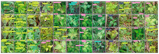
Figure 6.
Visual examples of original images and annotations.
Visual inspection of the sample images shows many frames with high instance density and frequent overlap or partial occlusion of individual plants. Some classes display large within-class variation in leaf shape, size, and color while other classes have very similar visual appearance, increasing the risk of inter-class confusion. Backgrounds are highly heterogeneous with mixtures of soil, grass, dead leaves, and debris that introduce texture noise and reduce contrast between weeds and surroundings. Capture conditions vary widely across images with differences in shooting distance, viewpoint, illumination and occasional motion blur, producing substantial scale and appearance variation.
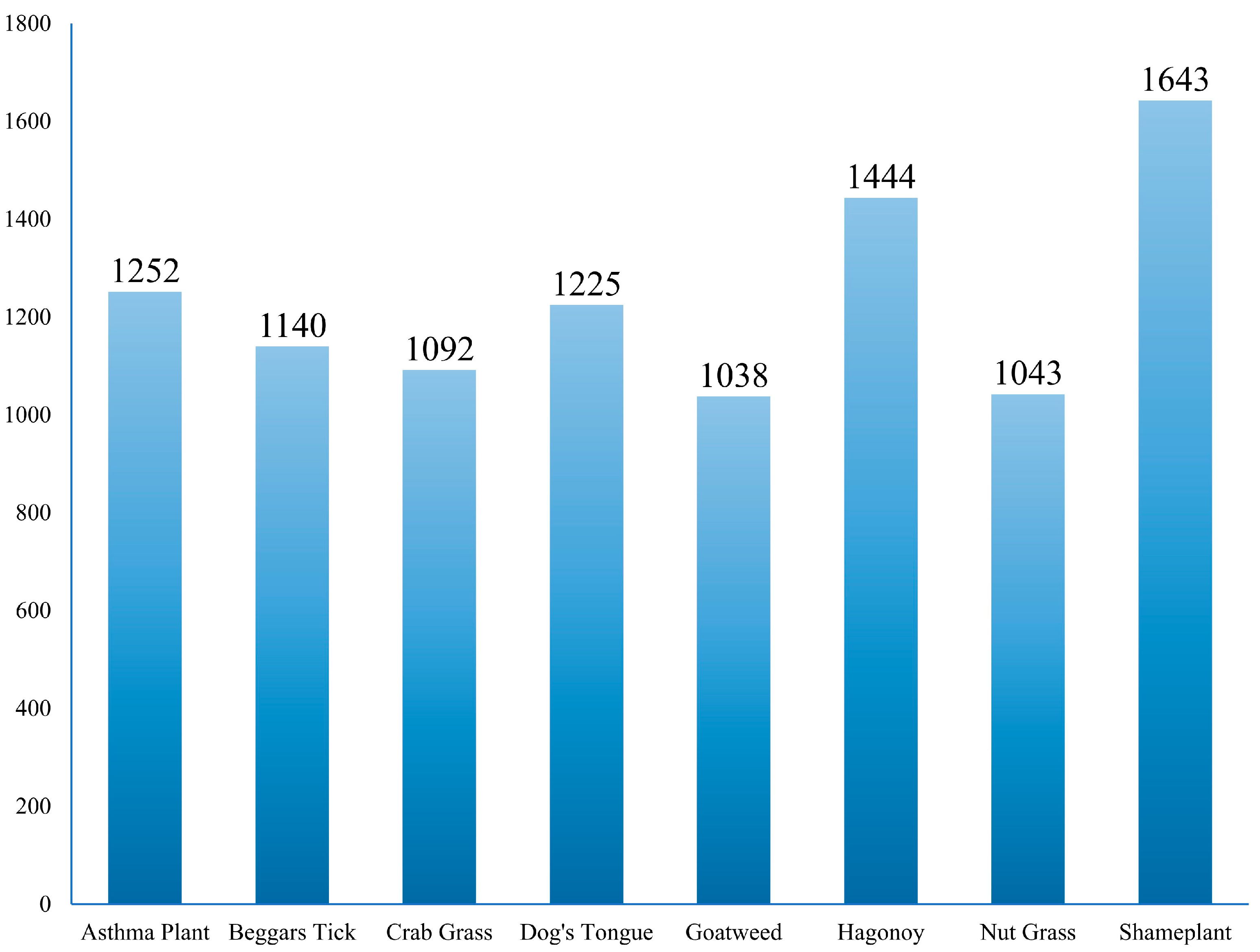
The training and validation sets are divided into a 9:1 ratio, with a total of 8331 images in the training set and 926 images in the validation set. The Weed dataset’s annotated categories include asthma plant, beggars tick, crab grass, dog’s tongue, goatweed, hagonoy, nut grass, and shameplant. The specific number of images in each category is shown in Figure 7.
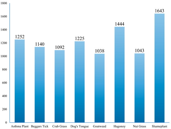
Figure 7.
Category image quantity statistics chart.
The Weed dataset covers southern China only, which may limit how well models trained on it generalize to other regions. Differences in species composition, background textures, soil, lighting, seasonal growth stages, and camera setups can create systematic shifts that reduce performance when the model is applied elsewhere. To help assess generalization, we supplemented experiments with external datasets collected in France and North Dakota in the United States. Reducing geographic bias will require broader sampling, targeted data augmentation, and domain-adaptive fine tuning before deploying the model in new areas.
4.2. Training Parameters
The model proposed in this paper is based on YOLO12-N and was trained from scratch for 300 epochs without using pretrained weights. For all subsequent experiments, the input image resolution was 640 pixels, the batch size was 16, and the number of workers was 8. The experimental platform was based on the Windows 11 operating system, with an AMD Ryzen 9 5900HX CPU with 64 GB of RAM and an NVIDIA GeForce RTX 3080 GPU with 16 GB of VRAM. The deep learning frameworks used were Torch 2.2.2 + cu121, torchvision 0.17.2 + cu121, CUDA 12.1.105, and cuDNN 8.9.7.29.
4.3. Evaluation Metrics
This paper uses common evaluation metrics to assess the weed detection performance of MIE-YOLO in precision agriculture, using both accuracy and speed. This division aims to focus on both accuracy and speed, allowing for a comprehensive evaluation of the detection results and highlighting both the model’s strengths and weaknesses.
Precision metrics primarily focus on the model’s detection accuracy and completeness, including Precision, Recall, F1 Score, and mAP (mean Average Precision). These metrics directly measure the model’s accuracy and comprehensiveness and are key to evaluating its performance in weed detection tasks. The formulas for calculating Precision, Recall, and F1 Score are as follows:
where P stands for Precision, R for Recall, and F for F1 Score. The TP in the formula represents the number of samples correctly predicted as positive, or the number of correctly detected objects. The FP represents the number of samples incorrectly predicted as positive, or the number of false positives. The FN represents the number of samples incorrectly predicted as negative, or the number of missed objects. The AP (Average Precision) is calculated by taking the area under the Precision-Recall Curve, and mAP is obtained by taking the average:
where P (R) is a curve showing the variation of Precision with Recall for each detection object. The n is the total number of detection categories, which is 8, including asthma plant, beggars tick, crab grass, dog’s tongue, goatweed, hagonoy, nut grass, and shameplant.
Speed metrics focus on the computational efficiency and running speed of the model during training and inference, reflecting the computational load and processing speed of the model under corresponding hardware conditions. Examples include the model’s Params (Parameters), FLOPs (Floating Point Operations), Size, and FPS (Frames Per Second). The standard FPS calculation formula is as follows:
where the standard FPS value is the reciprocal of the total time, which is the sum of the time for image preprocessing, model inference, and post-processing.
5. Discussion
5.1. Model Comparison Experiment Analysis
To comprehensively evaluate the performance of MIE-YOLO, it is compared with other classic object detection algorithms. All models were trained from scratch without pretrained weights and tested on an AMD Ryzen 9 5900HX CPU and an NVIDIA GeForce RTX 3080 GPU. The results of the model comparison experiments are shown in Table 1, which includes evaluation metrics such as Precision, Recall, F1 Score, mAP (mean Average Precision), Params (Parameters), FLOPs (Floating Point Operations), Size, and FPS (Frames Per Second).

Table 1.
Model comparison experiment results.
The MIE-YOLO uses the YOLO12-N algorithm as the benchmark model. The compared algorithms include YOLOv5-N (the minimum version of YOLOv5), YOLOv8-N (the minimum version of YOLOv8), YOLOv10-N (the minimum version of YOLOv10), YOLO11-N (the minimum version of YOLO11), YOLO12-N (the minimum version of YOLO12), YOLO13-N (the minimum version of YOLO13), RT-DETRv2-S (the minimum version of RT-DETRv2 [39]), and Deformable-DETR (Deformable Transformers for End-to-End Object Detection [40]).
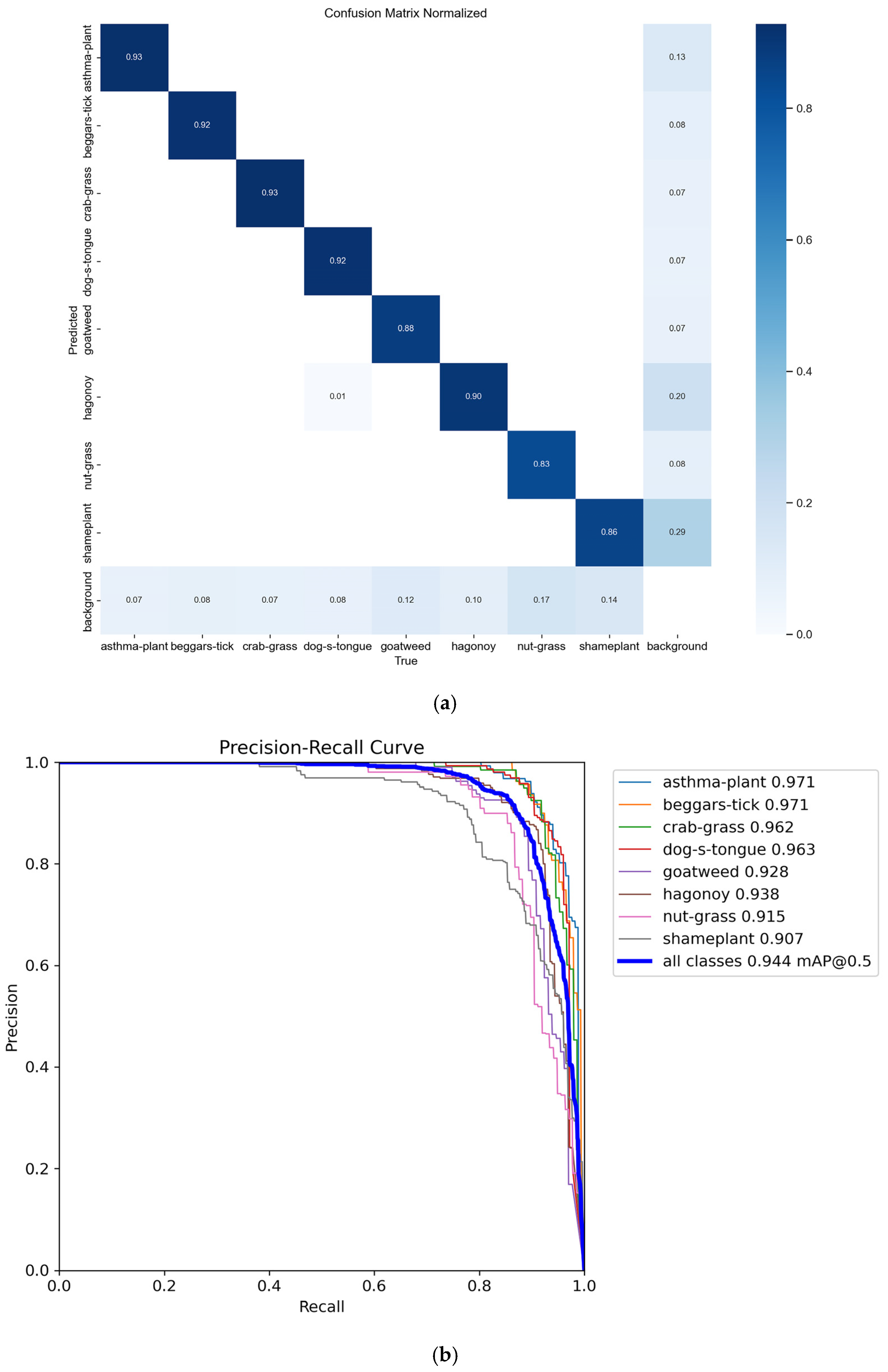
Experimental results show that MIE-YOLO achieves an F1 score of 89.3% and a mAP of 94.4%. Furthermore, MIE-YOLO requires only 1.76 M computational parameters, 5.4 G FLOPs, and a model size of 4.34 M, while running at a high speed of 66.2 FPS. Figure 8 shows the training results of MIE-YOLO, including the Confusion Matrix Normalized and Precision-Recall Curve.
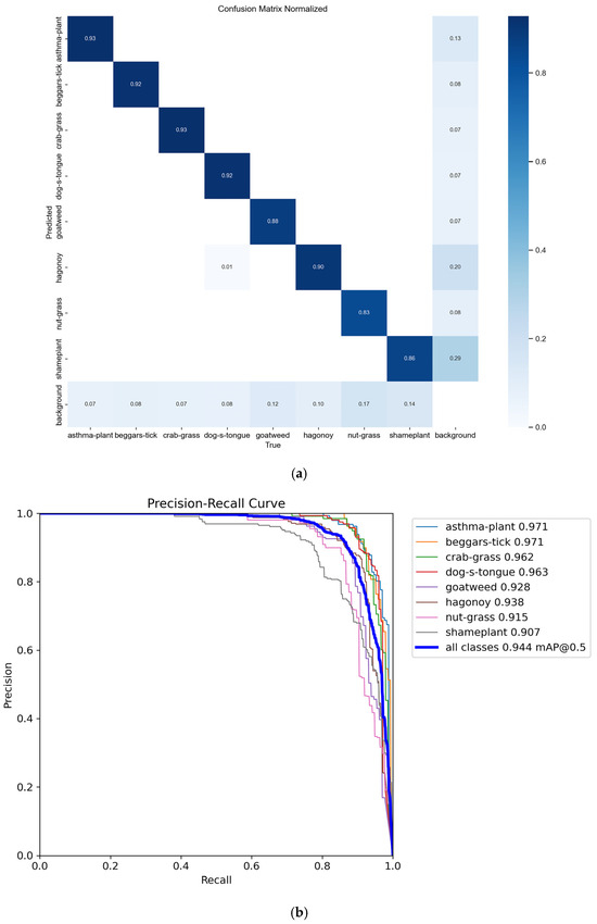
Figure 8.
Training results of MIE-YOLO: (a) Confusion Matrix Normalized, (b) PR Curve.
Compared to classic YOLO frameworks such as YOLOv5-N, YOLOv8-N, YOLOv10-N, and YOLO11-N, MIE-YOLO demonstrates superior accuracy and lightness. Compared to the latest YOLO13-N, MIE-YOLO achieves a 1.6% improvement in F1 score and a 1.6% increase in mAP. It also reduces computational parameters by 28.2%, FLOPs by 11.5%, and model size by 16.4%, while running 79.4% faster. As a result, MIE-YOLO achieves a better balance between accuracy and real-time performance, surpassing other YOLO family algorithms in detection performance.
Compared to the DETR family of models RT-DETRv2-S and Deformable-DETR, although MIE-YOLO has slightly lower accuracy, all computational parameters and model size are significantly smaller, and the running speed reaches 2 to 3 times the FPS. Although DETR-based models achieve slightly higher accuracy, they require substantially more parameters and computational resources, whereas MIE-YOLO delivers competitive performance with a much smaller model size and faster inference, making it more suitable for edge devices and mobile agricultural platforms.
Compared to the baseline YOLO12-N model, MIE-YOLO shows clear gains in both efficiency and accuracy. Precision rises from 91.9% to 94.5%, the F1 score improves from 87.4% to 89.3%, and mAP at 0.5 increases from 92.4% to 94.4%, while recall remains similar at 84.7% versus 83.4%. At the same time the model becomes substantially lighter and faster, with parameters falling from 2.51 M to 1.76 M, FLOPs dropping from 5.8 G to 5.4 G, model size shrinking from 5.23 M to 4.34 M, and inference speed climbing from 50.0 FPS to 66.2 FPS. Overall, MIE-YOLO does not trade accuracy for efficiency. Instead, it delivers higher detection performance while reducing computational cost and accelerating runtime, making it more suitable for real-time and resource-limited agricultural applications.
5.2. Module Ablation Experiment Analysis
To fully verify the contribution of each module in MIE-YOLO, ablation experiments were performed on all improved parts using YOLO12-N as the baseline model. Specifically, we added the MS-EIS architecture, the Add-CGLU pyramid network, and the DEC detection head to YOLO12-N, and combined it with the DS strategy to perform knowledge distillation on the overall architecture. The advantages of the model are demonstrated through a detailed discussion of the working principles. The results of the module ablation experiments are shown in Table 2, where module A represents the baseline YOLO12-N, module B represents the MS-EIS architecture, module C represents the Add-CGLU pyramid network, module D represents the DEC detection head, module E represents the ordinary single distillation strategy, and module F represents the DS knowledge distillation strategy.

Table 2.
Module ablation experiment results.
First, the MS-EIS architecture was introduced into the YOLO12-N baseline. Compared to the baseline, mAP improved by 0.7%, computational parameters were reduced by 19.9%, FLOPs were reduced by 5.2%, and model size was reduced by 12.6%, with a negligible impact on F1 score. This demonstrates that the MS-EIS architecture optimizes the model’s feature representation and task adaptability through multi-scale feature extraction, edge information enhancement, deep convolution operations, and dual region-focused attention.
Then, the Add-CGLU pyramid network was integrated into the YOLO12-N baseline. While FLOPs and model size increased slightly compared to the original, the F1 score and mAP values increased by 2.4% and 1.9%, respectively. The added computational cost comes from the local perception, additive token mixing, and gated convolutional operations that improve multi-scale representation, so the tradeoff is a modest rise in FLOPs and memory footprint in exchange for noticeably better detection accuracy. This makes Add-CGLU attractive when small increases in resource use are acceptable for gains in representational power and information transfer efficiency. This demonstrates that the Add-CGLU pyramid network improves the representational power and information transfer efficiency of multi-scale features through additive fusion and gating mechanisms.
Next, the DEC detection head was replaced in the YOLO12-N baseline. This resulted in a 1.8% improvement in F1 score and a 1.6% improvement in mAP. At the same time, computational parameters were reduced by 12.7%, FLOPs by 5.2%, and model size by 5.4%. The DEC detection head reduces parameters and FLOPs while improving accuracy by concentrating representational power where it matters and replacing some heavy static convolutions with lighter adaptive operations and shared parameters. These changes cut redundant weights and lower computational cost, which typically reduces memory use and can speed up inference on many devices. This demonstrates that the DEC detection head effectively reduces computational cost and parameter count through fine-grained feature enhancement, dynamic adaptive convolution, and shared parameter design.
Finally, knowledge distillation using the DS strategy was performed on the model incorporating all module improvements. Notably, the model’s lightness was not compromised, and the F1 score and mAP values increased by 0.1% and 1.1% respectively. This demonstrates that the DS strategy further improves the model’s detection accuracy and generalization performance while maintaining lightness.
By focusing on the last three rows of ablation experiments, the difference between single-stage distillation and the dual self-knowledge distillation proposed in this paper becomes apparent. Single-stage distillation raises precision from 91.0% to 92.1% and slightly increases mAP from 93.3% to 93.6% while leaving F1 unchanged at 89.2% and producing a small drop in recall to 86.4%. The DS strategy yields substantially larger gains, pushing precision to 94.5% and mAP to 94.4% with a marginal F1 increase to 89.3%, while keeping model lightness intact at 1.76 M parameters, 5.4 G FLOPs and 4.34 M size. These results indicate that DS produces stronger and more discriminative channel-level supervision than single-stage distillation, which sharpens decision boundaries and reduces false positives, hence the big precision and mAP improvements.
Ablation experiments demonstrate the effectiveness of both the lightweight improvements and the customized dual self-knowledge distillation strategy. MIE-YOLO successfully achieves a good balance between accuracy and real-time performance in real-time field weed identification and targeted spraying tasks in precision agriculture.
5.3. Model Generalization Experiment Analysis
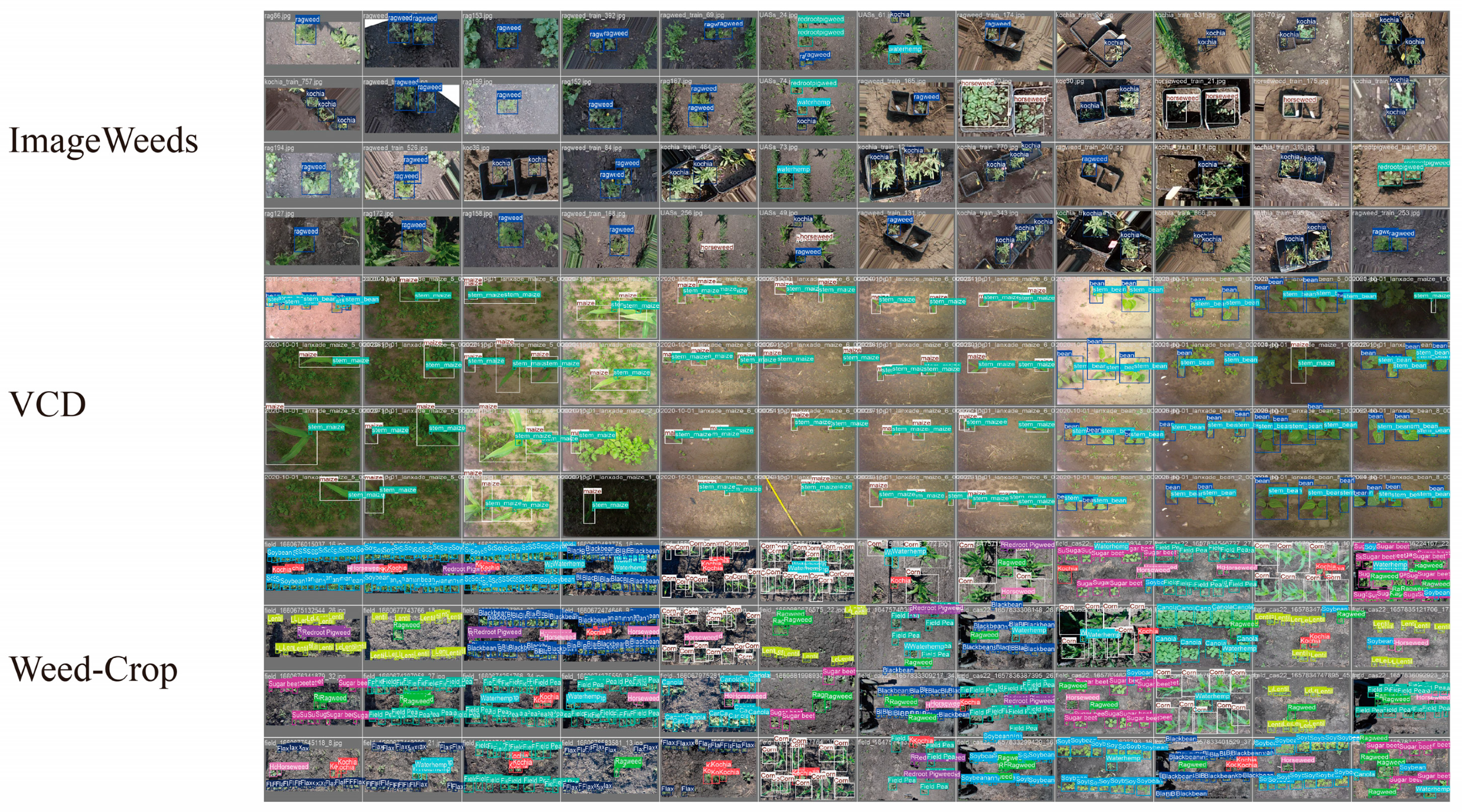
To extensively explore the robustness of MIE-YOLO, model generalization experiments were conducted on the ImageWeeds [41], VCD (Vegetable Crops Dataset) [42], and Weed-Crop [43] public datasets. The ImageWeeds dataset contains 3975 images showcasing five different weeds common in North Dakota, USA. Categories include ragweed, water hemp, horseweed, redroot pigweed, and kochia. The VCD dataset consists of 2801 images depicting soil conditions, weed infestation, and growth stages of various crops in North Dakota, USA. Categories include bean, stem bean, maize, stem maize, leek, and stem leek. The Weed-Crop dataset contains 1120 images featuring five weeds and eight crops from North Dakota, USA. Categories include black bean, canola, corn, field pea, flax, horseweed, kochia, lentil, ragweed, redroot pigweed, soybean, sugar beet, and water hemp. The corresponding sample images from the three datasets are shown in Figure 9.
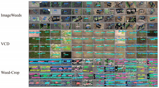
Figure 9.
Corresponding samples from the three datasets.
The images reveal several clear distributional traits that affect detection difficulty. Many photos contain multiple, densely packed instances with frequent overlap and partial occlusion, which increases the rate of missed detections and makes precise box regression harder. A large portion of targets are small relative to image size, leading to a heavy concentration of tiny bounding boxes and wide variation in object scales. Some classes exhibit high within-class variability in shape and color while other classes are visually similar to one another, raising the chance of inter-class confusion. Backgrounds are highly cluttered with mixed textures and debris, which reduces signal contrast and makes edge or texture cues less reliable.
The ImageWeeds dataset contains images with resolutions less than 640, while the VCD and Weed-Crop datasets contain images with resolutions greater than 640. Therefore, the generalization experiments can also verify the performance of MIE-YOLO at resolutions beyond 640. The comparison results of the evaluation indicators of MIE-YOLO and the baseline model on each dataset are shown in Table 3.

Table 3.
Model generalization experiment results.
On the ImageWeeds dataset, MIE-YOLO’s F1 score improved by 1.6% and its mAP increased by 0.2%. On the VCD dataset, the F1 score improved by 0.7% and its mAP increased by 0.5%. On the Weed-Crop dataset, the F1 score improved by 0.2% and its mAP increased by 1.3%. Furthermore, MIE-YOLO’s lightness was improved on all three datasets, with computational parameters reduced by 29.9%, FLOPs by 6.9%, and model size by 16.9%. Experimental results demonstrate that MIE-YOLO demonstrates excellent generalization capabilities, optimizing detection accuracy and robustness while maintaining a low computational cost and a compact architecture.
These results also reflect the robustness of the proposed method in a broader sense. Although the accuracy gains over external benchmarks are modest, the improvements are consistent across three datasets with very different scene characteristics, suggesting that MIE-YOLO adapts well to variations in imaging conditions, object density, and background clutter. More importantly, all key lightweight indicators show large margins of improvement, which means the model maintains or slightly improves accuracy while substantially reducing computational burden. This balance indicates that the architecture is not merely tuned for a single dataset but is structurally more efficient and less prone to overfitting, allowing it to retain performance even when computation, memory, or deployment constraints are tightened. In practical field applications where embedded devices or real-time systems are required, this combination of stable accuracy and significantly reduced complexity demonstrates stronger robustness than methods that achieve higher accuracy but rely on heavier architectures.
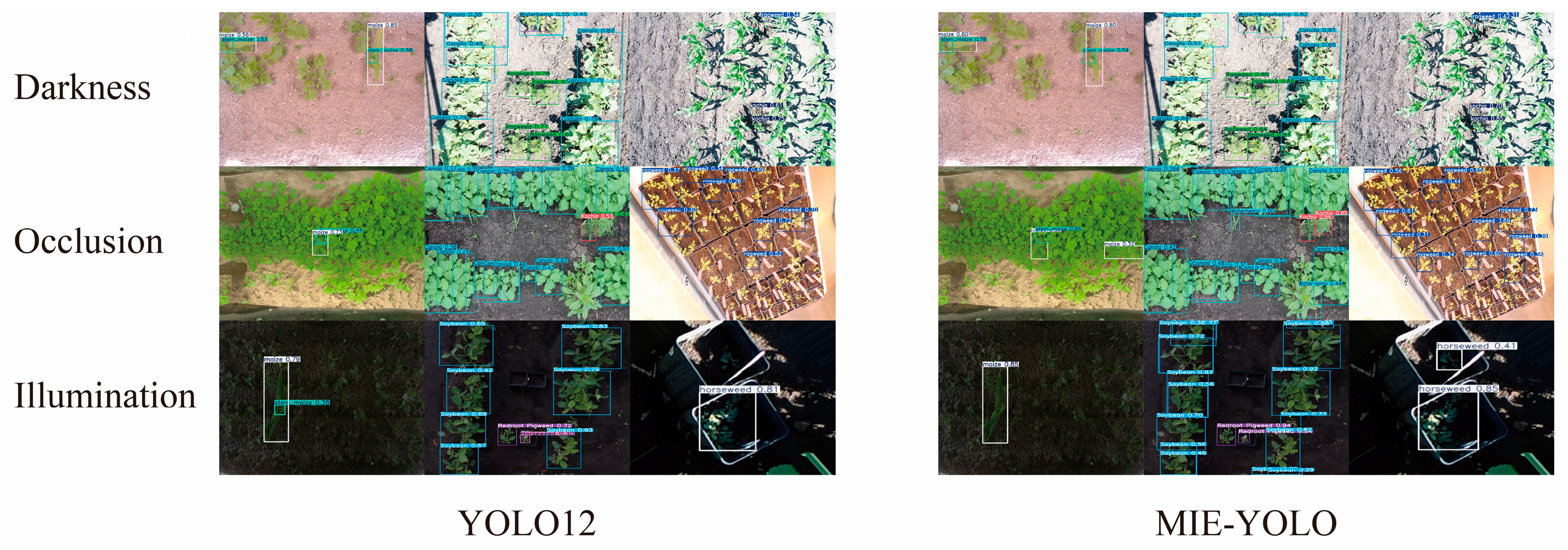
Figure 10 shows typical failure cases of YOLO12 and MIE-YOLO across three datasets, with extreme scenarios including darkness, occlusion, and illumination. The comparison image shows that MIE-YOLO produces noticeably higher confidence scores, tighter localization, and more complete detections across challenging conditions. For example, a horseweed instance that YOLO12 marked with low confidence near 0.41 is detected by MIE-YOLO with higher confidence near 0.85, and many small plants that are either missed or only weakly activated by YOLO12 appear as clear, high-confidence boxes in the MIE-YOLO output. Under darkness, heavy occlusion and varied illumination the right-hand results show denser, better-aligned bounding boxes around leaf margins and stems, while the left-hand results include more scattered low-confidence boxes and some missed targets. In short, MIE-YOLO identifies more targets, assigns higher probabilities to correct detections, and produces fewer spurious activations on background regions.

Figure 10.
Typical failure cases on generalized datasets.
These improvements matter in practice because higher confidence and improved localization reduce both missed detections and false positives, which in turn lowers the risk of ineffective spraying or unnecessary treatment in precision agriculture. The visual evidence also suggests MIE-YOLO is more robust to noisy conditions common in field data, maintaining detection quality where a baseline detector degrades. That robustness supports more reliable downstream decisions in deployment, especially on embedded platforms where model compactness and consistent output quality are critical.
5.4. Model Visualization Result Analysis
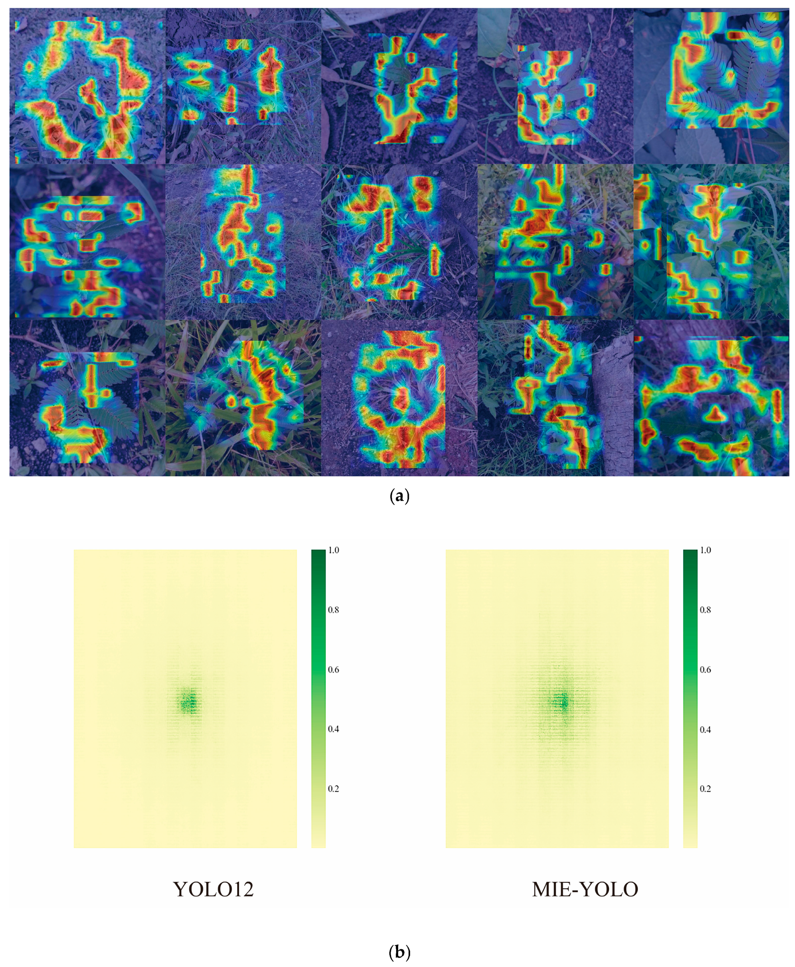
To directly demonstrate the transparency and clarity of MIE-YOLO, the model’s detection performance is visualized. The visualization results include the FH (Feature Heatmap) and the ERF (Effective Receptive Field), as shown in Figure 11. The FH projects intermediate features or responses based on target gradients back onto the input image and displays them as a normalized heatmap, visually revealing the model’s response strength to various spatial regions. The ERF, on the other hand, represents the actual contribution distribution of output units to input pixels. It is typically centered, approximately Gaussian, and smaller than the theoretical receptive field. It quantifies the effective scale at which the model aggregates contextual information.
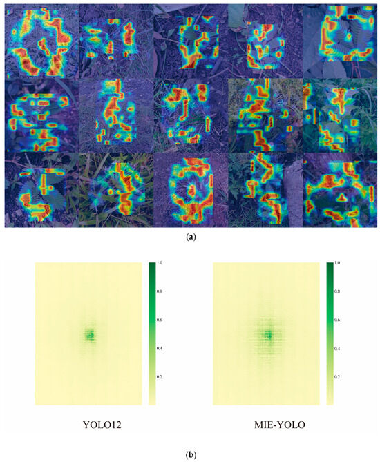
Figure 11.
Visualization results of MIE-YOLO: (a) Feature Heatmap, (b) Effective Receptive Field.
In the FH visualization, MIE-YOLO displays consistent high-response regions across multiple weed samples. These high responses are often aligned with leaf margins, stem nodes, or typical texture features of the plant, rather than background weeds or soil texture, demonstrating that the model is capable of achieving more accurate spatial attention despite complex occlusions and background interference. Compared with traditional detectors, the high-response blocks in the heat map are more concentrated and have clearer boundaries, and background false activations are significantly reduced. This reflects the robustness of MIE-YOLO in category judgment and local feature enhancement, which is conducive to improving the detection rate of weeds with approximate textures.
In the ERF visualization, the effective receptive field of MIE-YOLO shows a response distribution that is larger than that of YOLO12 and still has a significant center, indicating that the network can gather broader contextual information to support semantic inference while maintaining positioning accuracy. This more balanced spatial weight distribution helps leverage surrounding environmental cues for distinguishing weeds with significant scale and morphological differences, thereby improving detection stability and recall.
In summary, the visualization of FH and ERF demonstrates the advantages of MIE-YOLO in focusing on salient target features and expanding the effective receptive field to take into account both local details and global context. MIE-YOLO achieves a better balance between feature attention and spatial perception, demonstrating detection robustness and generalization capabilities in complex and diverse environments.
Despite these advantages, several practical limiting factors remain when deploying MIE-YOLO in real agricultural environments. Environmental variability is one of the primary challenges. Illumination changes caused by strong sunlight, cloud cover, or shadows from crops can introduce sharp intensity fluctuations that reduce feature stability, while wind-induced plant motion leads to deformation and blur that are difficult to fully model. Soil background differences, seasonal shifts in plant color, and variations in weed growth stages may also create domain gaps that exceed the range of the training data. These factors can weaken feature consistency and reduce the reliability of predictions when conditions deviate from those seen during training.
In addition, equipment integration constraints can significantly affect real-world performance. Mobile agricultural platforms often rely on low-power embedded processors, where thermal limitations, battery capacity, and bandwidth restrictions may reduce the achievable inference speed compared with laboratory settings. Camera sensors with lower dynamic range or variable mounting angles may further distort feature distribution, and vibration from field machinery can degrade image quality and temporal consistency. These limitations indicate that, although MIE-YOLO shows strong robustness and generalization in controlled evaluations, additional adaptation strategies such as dynamic exposure adjustment, temporal stabilization, or domain-adaptive fine tuning are needed to ensure consistently reliable performance in large scale agricultural deployment. Table 4 shows the actual inference speed and resource consumption of MIE-YOLO on embedded devices or mobile platforms.

Table 4.
Mobile platform deployment results.
Table 4 shows MIE-YOLO achieves disproportionately high speed relative to reported GPU performance on mobile SoCs. On Snapdragon 8 Elite the model runs at 56.3% of RTX 3080 speed while the device GPU performance is 36.6%, a gap of 19.7 percentage points. On Dimensity 9400 the speed is 53.3% versus GPU performance of 36.5%, a gap of 16.8 points. On Apple M4 the speed is 55.3% versus GPU performance of 35.6%, a gap of 19.7 points. Even on the lower end, A18 Pro the speed is 44.1% while GPU performance is 21.1%, a gap of 23.0 points. Inference stays in the mid-20 ms range yielding roughly 29 to 37 FPS and preprocessing and postprocessing overheads are minimal so most runtime is efficient neural inference. These runtime advantages are supported by reductions in parameters by 29.9% FLOPs by 6.9% and model size by 17.0 which lower memory footprint and compute demand. Modest reported GPU utilization leaves headroom for multitasking and battery saving which is important for field deployment in battery-powered sprayers and drones. Together these facts demonstrate that MIE-YOLO attains higher real-time throughput than raw device performance would predict and is therefore well suited for resource-constrained embedded and mobile platforms while still allowing further gains from vendor acceleration quantization or targeted pruning.
6. Conclusions
This paper proposes a multi-scale information-enhanced weed detection algorithm, MIE-YOLO, for precision agriculture. By introducing a novel MS-EIS (Multi Scale-Edge Information Select) architecture, an Add-CGLU (Additive-Convolutional Gated Linear Unit) pyramid network, and a DEC (Detail-Enhanced Convolution) detection head, MIE-YOLO employs a DS (Double Self-Knowledge Distillation) strategy to distill knowledge across the entire network. Experimental results on a custom Weed dataset demonstrate that MIE-YOLO improves the F1 score by 1.9% and the mean average prediction accuracy by 2.0%. Furthermore, MIE-YOLO reduces computational parameters by 29.9%, FLOPs by 6.9%, and model size by 17.0%, achieving a runtime speed of 66.2 FPS. These results demonstrate that MIE-YOLO achieves the efficient and accurate recognition of multi-class, densely distributed, and small weed targets.
Despite these gains, MIE-YOLO has several important limitations that need further study. Its performance under extreme lighting and motion blur is not fully validated because the MS-EIS module depends on edge and texture cues that can be degraded in such conditions. Severe occlusion and dense overlap between weeds and crops remain challenging since DEC enhancements cannot always recover fully occluded instances. Fine grained similarity between some crops and weeds causes false positives and indicates a need for more discriminative features or class-balanced training. Practical concerns such as annotation noise, sensitivity to hyperparameters, and limited field trials may also limit real world translation. Future work will therefore prioritize expanding and diversifying the dataset and performing targeted model compression and hardware acceleration tests to validate deployment. MIE-YOLO is expected to achieve large-scale deployment in complex farmland environments through deep integration with automated weeding machinery and precision spraying systems, and provide strong support for improving crop yields and pesticide use efficiency.
Author Contributions
Conceptualization, Y.X. and D.D.; methodology, Y.X.; software, Y.X.; validation, Z.H., Y.X. and D.D.; formal analysis, Y.X.; investigation, Z.H.; resources, Z.H.; data curation, Y.X.; writing—original draft preparation, Y.X.; writing—review and editing, Z.H.; visualization, Y.X.; supervision, D.D.; project administration, Y.X.; funding acquisition, Z.H. All authors have read and agreed to the published version of the manuscript.
Funding
This research received no external funding.
Institutional Review Board Statement
Not applicable.
Informed Consent Statement
Not applicable.
Data Availability Statement
The original contributions presented in this study are included in the article. Further inquiries can be directed to the corresponding authors.
Acknowledgments
The authors would like to acknowledge the College of Life Science and Technology, Guangxi University for providing data support.
Conflicts of Interest
The authors declare no conflicts of interest.
References
- Xie, Y.; Du, D.; Bi, M. YOLO-ACE: A Vehicle and Pedestrian Detection Algorithm for Autonomous Driving Scenarios Based on Knowledge Distillation of YOLOv10. IEEE Internet Things J. 2025, 12, 30086–30097. [Google Scholar] [CrossRef]
- Xie, Y.; Du, D.; Liu, Y. RE-YOLO: Vehicle Detector Based on Knowledge Distillation YOLOv8 for Autonomous Driving Scenarios. J. Comput. Civ. Eng. 2025, 39, 04025084. [Google Scholar] [CrossRef]
- Du, D.; Xie, Y. Vehicle and Pedestrian Detection Algorithm in an Autonomous Driving Scene Based on Improved YOLOv8. J. Transp. Eng. Part A Systems 2025, 151, 04024095. [Google Scholar] [CrossRef]
- Xie, Y.; Du, D.; Wang, Z.; Liu, Y.; Bi, M. YOLO-SFT: Road Damage Detection Algorithm Based on Feature Diffusion. J. Transp. Eng. Part B Pavements 2025, 151, 04025004. [Google Scholar] [CrossRef]
- Girshick, R.; Donahue, J.; Darrell, T.; Malik, J. Rich Feature Hierarchies for Accurate Object Detection and Semantic Segmentation. In Proceedings of the 2014 IEEE Conference on Computer Vision and Pattern Recognition, Columbus, OH, USA, 23–28 June 2014; pp. 580–587. [Google Scholar]
- He, K.; Zhang, X.; Ren, S.; Sun, J. Spatial Pyramid Pooling in Deep Convolutional Networks for Visual Recognition. IEEE Trans. Pattern Anal. Mach. Intell. 2015, 37, 1904–1916. [Google Scholar] [CrossRef]
- Girshick, R. Fast R-CNN. In Proceedings of the 2015 IEEE International Conference on Computer Vision (ICCV), Santiago, Chile, 7–13 December 2015; pp. 1440–1448. [Google Scholar]
- Ren, S.; He, K.; Girshick, R.; Sun, J. Faster R-CNN: Towards Real-Time Object Detection with Region Proposal Networks. IEEE Trans. Pattern Anal. Mach. Intell. 2017, 39, 1137–1149. [Google Scholar] [CrossRef]
- Lin, T.-Y.; Dollar, P.; Girshick, R.; He, K.; Hariharan, B.; Belongie, S. Feature Pyramid Networks for Object Detection. In Proceedings of the 2017 IEEE Conference on Computer Vision and Pattern Recognition (CVPR), Honolulu, HI, USA, 21–26 July 2017; pp. 936–944. [Google Scholar]
- Redmon, J.; Divvala, S.; Girshick, R.; Farhadi, A. You Only Look Once: Unified, Real-Time Object Detection. In Proceedings of the 2016 IEEE Conference on Computer Vision and Pattern Recognition (CVPR), Las Vegas, NV, USA, 27–30 June 2016; pp. 779–788. [Google Scholar]
- Liu, W.; Anguelov, D.; Erhan, D.; Szegedy, C.; Reed, S.; Fu, C.-Y.; Berg, A.C. SSD: Single Shot MultiBox Detector. In Computer Vision—ECCV 2016; Leibe, B., Matas, J., Sebe, N., Welling, M., Eds.; Springer International Publishing: Cham, Switzerland, 2016; Volume 9905, pp. 21–37. ISBN 9783319464473. [Google Scholar]
- Lin, T.-Y.; Goyal, P.; Girshick, R.; He, K.; Dollar, P. Focal Loss for Dense Object Detection. In Proceedings of the 2017 IEEE International Conference on Computer Vision (ICCV), Venice, Italy, 22–29 October 2017; pp. 2999–3007. [Google Scholar]
- Law, H.; Deng, J. CornerNet: Detecting Objects as Paired Keypoints. In Computer Vision—ECCV 2018; Ferrari, V., Hebert, M., Sminchisescu, C., Weiss, Y., Eds.; Springer International Publishing: Cham, Switzerland, 2018; Volume 11218, pp. 765–781. ISBN 9783030012632. [Google Scholar]
- Duan, K.; Bai, S.; Xie, L.; Qi, H.; Huang, Q.; Tian, Q. CenterNet: Keypoint Triplets for Object Detection. In Proceedings of the 2019 IEEE/CVF International Conference on Computer Vision (ICCV), Seoul, Republic of Korea, 27–28 October 2019; pp. 6568–6577. [Google Scholar]
- Carion, N.; Massa, F.; Synnaeve, G.; Usunier, N.; Kirillov, A.; Zagoruyko, S. End-to-End Object Detection with Transformers. In Computer Vision—ECCV 2020; Vedaldi, A., Bischof, H., Brox, T., Frahm, J.-M., Eds.; Springer International Publishing: Cham, Switzerland, 2020; Volume 12346, pp. 213–229. ISBN 9783030584511. [Google Scholar]
- Wang, C.-Y.; Yeh, I.-H.; Mark Liao, H.-Y. YOLOv9: Learning What You Want to Learn Using Programmable Gradient Information. In Computer Vision—ECCV 2024; Leonardis, A., Ricci, E., Roth, S., Russakovsky, O., Sattler, T., Varol, G., Eds.; Springer Nature Switzerland: Cham, Switzerland, 2025; Volume 15089, pp. 1–21. ISBN 9783031727504. [Google Scholar]
- Wang, A.; Chen, H.; Liu, L.; Chen, K.; Lin, Z.; Han, J.; Ding, G. YOLOv10: Real-Time End-to-End Object Detection. arXiv 2024, arXiv:2405.14458. [Google Scholar]
- Khanam, R.; Hussain, M. YOLOv11: An Overview of the Key Architectural Enhancements. arXiv 2024, arXiv:2410.17725. [Google Scholar] [CrossRef]
- Tian, Y.; Ye, Q.; Doermann, D. YOLOv12: Attention-Centric Real-Time Object Detectors. arXiv 2025, arXiv:2502.12524. [Google Scholar]
- Lei, M.; Li, S.; Wu, Y.; Hu, H.; Zhou, Y.; Zheng, X.; Ding, G.; Du, S.; Wu, Z.; Gao, Y. YOLOv13: Real-Time Object Detection with Hypergraph-Enhanced Adaptive Visual Perception. arXiv 2025, arXiv:2506.17733. [Google Scholar]
- Deng, L.; Miao, Z.; Zhao, X.; Yang, S.; Gao, Y.; Zhai, C.; Zhao, C. HAD-YOLO: An Accurate and Effective Weed Detection Model Based on Improved YOLOV5 Network. Agronomy 2024, 15, 57. [Google Scholar] [CrossRef]
- Wang, X.; Wang, Q.; Qiao, Y.; Zhang, X.; Lu, C.; Wang, C. Precision Weed Management for Straw-Mulched Maize Field: Advanced Weed Detection and Targeted Spraying Based on Enhanced YOLO V5s. Agriculture 2024, 14, 2134. [Google Scholar] [CrossRef]
- Tao, T.; Wei, X. STBNA-YOLOv5: An Improved YOLOv5 Network for Weed Detection in Rapeseed Field. Agriculture 2024, 15, 22. [Google Scholar] [CrossRef]
- Zhang, C.; Liu, J.; Li, H.; Chen, H.; Xu, Z.; Ou, Z. Weed Detection Method Based on Lightweight and Contextual Information Fusion. Appl. Sci. 2023, 13, 13074. [Google Scholar] [CrossRef]
- Hu, J.; Gong, H.; Li, S.; Mu, Y.; Guo, Y.; Sun, Y.; Hu, T.; Bao, Y. Cotton Weed-YOLO: A Lightweight and Highly Accurate Cotton Weed Identification Model for Precision Agriculture. Agronomy 2024, 14, 2911. [Google Scholar] [CrossRef]
- Chen, Z.; Chen, B.; Huang, Y.; Zhou, Z. GE-YOLO for Weed Detection in Rice Paddy Fields. Appl. Sci. 2025, 15, 2823. [Google Scholar] [CrossRef]
- Zheng, L.; Yi, J.; He, P.; Tie, J.; Zhang, Y.; Wu, W.; Long, L. Improvement of the YOLOv8 Model in the Optimization of the Weed Recognition Algorithm in Cotton Field. Plants 2024, 13, 1843. [Google Scholar] [CrossRef]
- Shuai, Y.; Shi, J.; Li, Y.; Zhou, S.; Zhang, L.; Mu, J. YOLO-SW: A Real-Time Weed Detection Model for Soybean Fields Using Swin Transformer and RT-DETR. Agronomy 2025, 15, 1712. [Google Scholar] [CrossRef]
- Umar, U.M.; Ünal, Z.; Gulzar, Y.; Şen, B.; Alkanan, M.; Mir, M.S. Deep Learning-Based Classification of Lavender for Enhanced Cultivation and Essential Oil Quality Management. J. Essent. Oil Bear. Plants 2025, 28, 1063–1085. [Google Scholar] [CrossRef]
- Gulzar, Y. Papaya Leaf Disease Classification Using Pre-Trained Deep Learning Models: A Comparative Study. Appl. Fruit Sci. 2025, 67, 287. [Google Scholar] [CrossRef]
- Gulzar, Y. PapNet: An AI-Driven Approach for Early Detection and Classification of Papaya Leaf Diseases. Appl. Fruit Sci. 2025, 67, 256. [Google Scholar] [CrossRef]
- Han, H.; Bhatti, U.A.; Gulzar, Y.; Alkanan, M.; Mir, M.S.; Hao, T. Precision Agricultural Techniques for Coconut Disease Segmentation Using Enhanced Remote Sensing Images. Spat. Inf. Res. 2025, 33, 50. [Google Scholar] [CrossRef]
- Cui, Y.; Ren, W.; Cao, X.; Knoll, A. Focal Network for Image Restoration. In Proceedings of the 2023 IEEE/CVF International Conference on Computer Vision (ICCV), Paris, France, 1–6 October 2023; pp. 12955–12965. [Google Scholar]
- Zhang, T.; Li, L.; Zhou, Y.; Liu, W.; Qian, C.; Hwang, J.-N.; Ji, X. CAS-ViT: Convolutional Additive Self-Attention Vision Transformers for Efficient Mobile Applications. arXiv 2024, arXiv:2408.03703. [Google Scholar]
- Shi, D. TransNeXt: Robust Foveal Visual Perception for Vision Transformers. In Proceedings of the 2024 IEEE/CVF Conference on Computer Vision and Pattern Recognition (CVPR), Seattle, WA, USA, 16–22 June 2024; pp. 17773–17783. [Google Scholar]
- Chen, Z.; He, Z.; Lu, Z.-M. DEA-Net: Single Image Dehazing Based on Detail-Enhanced Convolution and Content-Guided Attention. IEEE Trans. Image Process. 2024, 33, 1002–1015. [Google Scholar] [CrossRef]
- Hinton, G.; Vinyals, O.; Dean, J. Distilling the Knowledge in a Neural Network. arXiv 2015, arXiv:1503.02531. [Google Scholar] [CrossRef]
- Shu, C.; Liu, Y.; Gao, J.; Yan, Z.; Shen, C. Channel-Wise Knowledge Distillation for Dense Prediction. In Proceedings of the 2021 IEEE/CVF International Conference on Computer Vision (ICCV), Montreal, QC, Canada, 10–17 October 2021; pp. 5291–5300. [Google Scholar]
- Lv, W.; Zhao, Y.; Chang, Q.; Huang, K.; Wang, G.; Liu, Y. RT-DETRv2: Improved Baseline with Bag-of-Freebies for Real-Time Detection Transformer. arXiv 2024, arXiv:2407.17140. [Google Scholar]
- Zhu, X.; Su, W.; Lu, L.; Li, B.; Wang, X.; Dai, J. Deformable DETR: Deformable Transformers for End-to-End Object Detection. arXiv 2021, arXiv:2010.04159. [Google Scholar]
- Rai, N.; Mahecha, M.V.; Christensen, A.; Quanbeck, J.; Zhang, Y.; Howatt, K.; Ostlie, M.; Sun, X. Multi-Format Open-Source Weed Image Dataset for Real-Time Weed Identification in Precision Agriculture. Data Brief 2023, 51, 109691. [Google Scholar] [CrossRef]
- Lac, L.; Keresztes, B.; Louargant, M.; Donias, M.; Da Costa, J.-P. An Annotated Image Dataset of Vegetable Crops at an Early Stage of Growth for Proximal Sensing Applications. Data Brief 2022, 42, 108035. [Google Scholar] [CrossRef] [PubMed]
- Upadhyay, A.; Mahecha, M.V.; Mettler, J.; Howatt, K.; Aderholdt, W.; Ostlie, M.; Sun, X. Weed-Crop Dataset in Precision Agriculture: Resource for AI-Based Robotic Weed Control Systems. Data Brief 2025, 60, 111486. [Google Scholar] [CrossRef]
Disclaimer/Publisher’s Note: The statements, opinions and data contained in all publications are solely those of the individual author(s) and contributor(s) and not of MDPI and/or the editor(s). MDPI and/or the editor(s) disclaim responsibility for any injury to people or property resulting from any ideas, methods, instructions or products referred to in the content. |
© 2026 by the authors. Licensee MDPI, Basel, Switzerland. This article is an open access article distributed under the terms and conditions of the Creative Commons Attribution (CC BY) license.

