Utility of Domain Adaptation for Biomass Yield Forecasting

Abstract

Previous work used machine learning (ML) to estimate past and current alfalfa yields and showed that domain adaptation (DA) with data synthesis shows promise in classifying yields as high, medium, or low. The current work uses similar techniques to forecast future alfalfa yields. A novel technique is proposed for forecasting alfalfa time series data that exploits stationarity and predicts differences in yields rather than the yields themselves. This forecasting technique generally provides more accurate forecasts than the established ARIMA family of forecasters for both univariate and multivariate time series. Furthermore, this ML-based technique is potentially easier to use than the ARIMA family of models. Also, previous work is extended by showing that DA with data synthesis also works well for predicting continuous values, not just for classification. The novel scale-invariant tabular synthesizer (SITS) is proposed, and it is competitive with or superior to other established synthesizers in producing data that trains strong models. This synthesis algorithm leads to R scores over 100% higher than an established synthesizer in this domain, while ML-based forecasters beat the ARIMA family with symmetric mean absolute percent error (sMAPE) scores as low as 12.81%. Finally, ML-based forecasting is combined with DA (ForDA) to create a novel pipeline that improves forecast accuracy with sMAPE scores as low as 9.81%. As alfalfa is crucial to the global food supply, and as climate change creates challenges with managing alfalfa, this work hopes to help address those challenges and contribute to the field of ML.

1. Introduction

As the Earth’s climate changes, its population grows, and environments and weather patterns become increasingly unpredictable, problems in efficient crop production are among the most important to solve. Alfalfa, a particularly important livestock feed, has been called “Queen of the forage crops”, and it is the crop of focus for the current study [1]. Alfalfa is crucial to global food security because it is a valuable, sustainable, and protein-rich livestock feed as well as a nutritious food for people worldwide. In other words, alfalfa is not just food for people, but food for people’s food. Meanwhile, climate change directly threatens alfalfa’s efficient and sustainable cultivation [2]. The importance of alfalfa is evidenced by the attention it receives from many land-grant universities, which cultivate alfalfa and collect and publish data on it in the form of variety trials. These variety trials, along with weather data, are the data underlying the current work.

Meanwhile, in 2015, the United Nations (U.N.) agreed on and published the “Sustainable Development Goals”, 17 goals that “are the blueprint to achieve a better and more sustainable future for all. They address the global challenges we face, including poverty, inequality, climate change, environmental degradation, peace and justice.” Most specifically, the current work attempts to contribute toward “Goal 2: Zero Hunger,” and “Goal 13: Climate Action” [3]. Sadly, we are not yet on track to achieve Goal 2 [4], but it is our fervent hope to contribute towards this goal. Existing methods, such as the ARIMA family of algorithms and deep neural networks are not sufficient for the goals of this paper. One of the end goals of this research is to provide a lightweight and accessible application for farmers as end-users. ARIMA family algorithms and neural networks both require large datasets for training. This is problematic as agricultural datasets are often not large, as we highlight later in this paper. We can sidestep this using synthetic data generated via our novel SITS algorithm and XGBoost. Deep neural networks often require a high quantity of expensive computational resources on which to train, while our models do not require access to GPUs. ARIMA algorithms are also somewhat subjective in progress evaluations, and parameters [5]. The methods proposed here are more objective and less limited. The current work’s technical focus is forecasting alfalfa yield data as time series. Domain adaptation (DA) was also researched along the way as a steppingstone between crop yield estimation and forecasting. This work is presented as three phases. The first phase is DA, the second is ML-based forecasting, and the third phase is combining ML-based forecasting with DA.

To offer intuitive definitions of univariate and multivariate, time series data may consist of only one feature, which is known as univariate time series, or it may have several features, which is known as multivariate time series [6]. When the features do not directly cause one another, they may be known as exogenous features or variables, and when they do cause one another, they may be referred to as endogenous features or variables, roughly speaking. For example, the current work focuses on precipitation, solar radiation, temperature, and yield, none of which directly cause each other, though solar radiation affects temperature somewhat. On the other hand, yield is directly affected by the size of the growing site, so that would be more of an endogenous variable. Lütkepohl offers a formal mathematical definition of exogenous and endogenous variables in his book on time series [7]. The current work proposes both univariate and multivariate forecaster versions and compares them to the traditional family of autoregressive integrated moving average (ARIMA) statistical forecasting models. The proposed univariate ML-based forecaster was compared to the univariate ARIMA and seasonal ARIMA (SARIMA) models, and the multivariate ML-based forecaster was compared to the multivariate SARIMA with exogenous variables model (SARIMAX). ARIMA models are widely used in time series forecasting due to their ability to model trends and seasonality through autoregressive and moving average components [8]. However, our results show that the proposed univariate ML-based forecaster produced more accurate forecasts than the ARIMA family, as detailed in the Results Section, with symmetric mean absolute percent errors (sMAPEs) as low as 16.94% with the proposed forecaster versus a best of 34.67% with SARIMA. Univariate and multivariate models were compared, showing an improvement in sMAPE from 16.94% to 12.81% when exogenous variables were included in the ML-based forecaster, while SARIMAX produced a sMAPE of 28.08%.

The final phase of this work combines the proposed ML-based forecasting technique with DA using SITS, and shows the most promising sMAPE scores of all, as low as 9.81% at best. Experiments in earlier work showed that DA may be helpful when target data are scarce, and they focused on the very difficult problem of using data with one distribution to estimate that of a different distribution. As research progressed to the current work, results became very promising, but the problem became easier in that local training was used after the initial pretraining step, so even though forecasting is more challenging than estimating the past and present, the local training helps it produce good results.

The current work makes four significant contributions. First, a novel DA technique is proposed that combines data synthesis with pretraining an XGBoost model and substantially increases estimation accuracy. Second, a novel data synthesis algorithm is proposed that shows improvement over established models. Third, a novel ML-based forecasting algorithm is proposed that exploits stationarity. Fourth, the proposed ML-based forecasting technique is combined with the proposed DA pipeline to produce more accurate forecasters.

2. Related Work

Prior approaches in agricultural forecasting often relied on isolated data streams, mostly utilizing either textual data from reports or satellite imagery [9,10] in isolation to predict crop yields. A survey by Satore et al. focused on a hybrid approach combining NASA remote sensing data, built administrative boundaries to separate areas of interest, and used a combination of historical satellite imagery and county-level National Agricultural Statistics Service (NASS) to build a dataset for training and validation of the model. While these approaches have made valuable contributions, they faced challenges in capturing all trends present in textual data, leading them to incorporate additional data sources into their methodologies. To address these challenges, they introduced empirical density functions derived from remote sensing data, capturing the distribution of spectral signatures across different crop types. Utilizing multi-dimensional scaling, they transformed these high-dimensional density functions into a lower-dimensional space, generating artificial covariates that retain essential information while simplifying analysis. These artificial covariates, representing distilled, critical features of the agricultural landscape, were then used to train machine learning models. The models then underwent training and validation, leveraging the constructed dataset that integrates the artificial covariates with NASS official statistics. This innovative approach, while effective, still encountered limitations in capturing the entirety of textual data trends [11].

Building upon this, Gro Intelligence has implemented a real-time application of crop yield predictions to predict corn yields in the United States from diverse data sources. Cai et al.’s approach is a practical execution of the strategies proposed by Satore et al., taking the integration of diverse data sources to the next level by integrating a multi-level machine learning model and leveraging an extensive range of data sources to predict end-of-season corn yields in the United States from 2001 to 2016. Similarly to previous approaches, they faced challenges in fully capturing all trends present in textual data, prompting them to adopt a hybrid approach. This model showcases a sophisticated blend of algorithms, applying knowledge of physiological processes for temporal feature selection, achieving great precision in intra-season forecasts, even in years with anomalous growing conditions. It was back tested between 2000 and 2015, demonstrating the model’s capacity to predict national yield within approximately 2.69% of the actual yield by mid-August. In its first operational year during 2016, the model performed on par with the USDA’s forecasts and commercially available private yield models. At the county level, it could predict 77% of the variation in final yield using data through the beginning of August, with this figure improving to 80% by the beginning of October. Moreover, Gro Intelligence’s methodology enhances the original concept by focusing on the temporal aspects of data collection and analysis, allowing for intra-season adjustments to forecasts based on newly acquired data points. This real-time adaptability ensures that the predictive models are sensitive to sudden changes in weather patterns, crop conditions, and other critical factors affecting yield outcomes. Despite these advancements, the approach still encounters challenges in fully capturing the complexity of textual data trends [12].

In previous work, the current authors presented results of DA with synthesis classification experiments performed using a conditional tabular generative adversarial network (CTGAN) and tabular variational autoencoder (TVAE) proposed by Park et al. [13], and that work provided a more detailed description of those networks [14]. While these synthesizers motivated the current use of data synthesis in precision agriculture, SITS produced the best results in the current work.

Kastens et al. studied crop yield time series forecasting using computer vision with masking, and while they report relative success, they do not explore any forecasting models beyond linear regression, and they do not compare their results to other forecasting models like the ARIMA family. They forecast metric tons per acre for corn, wheat, and soybean, but not tons per acre of alfalfa, and their metric of choice is mean absolute error (MAE), so it is difficult to compare the quality of their results to the current work’s. Kasten et al. claim to require at least 11 years of training data to train a strong forecaster, while the current work produces very low sMAPE scores with as few as six years of training data. Finally, their work is another example of computer vision, which involves extra complexity and expensive equipment beyond the needs of the current work [15]. Choudhury and Jones compared statistical forecasting techniques to forecast maize yields in Ghana, and they report a significant contribution in this domain with mean squared errors (MSEs) as low as 0.03 metric tons per hectare using an autoregressive (AR) model, though that text does not appear to address or explain the table that features this metric. Furthermore, they emphasize coefficient of determination (R²) scores in that paper’s discussion, which experiments in the current work have shown to not be a very reliable metric for measuring the quality of time series forecasts. The Results and Discussion Sections herein elaborate on this. Choudhury and Jones also limit their results to those from AR models and a few varieties of exponential smoothing, though they refer to it as an autoregressive and moving average (ARMA) model in their discussions, and they do not explore multivariate models [16]. Bose et al. propose a spiking neural network (SNN) to forecast winter wheat crop yields from multispectral imaging time series data, and the SNN “encodes temporal information by transforming input data into trains of spikes that represent time-sensitive events” into a positive or negative binary value called a spike. That work reports high average prediction accuracies and R scores, and it reports beating linear regression (LR), k-nearest neighbors (KNNs), and support vector regression (SVR), but they do not compare their model to SARIMAX or other non-ML multivariate models. Most importantly, that work forecasts only one yield per year, six weeks into the future, while the current work forecasts three or four yields per year usually at least nine months into the future. Also, their R score appears to be calculated over the 14 years of predictions, so it bears little relevance to any R scores reported in the current work, which are calculated from a year’s forecast of several time points and the true values for that year. Also, although Bose et al. report that their SNN produces MAE scores as low as 0.24 tons per hectare, the current work’s ML-based technique produces MAE scores as low as 0.15 tons per acre, which is competitive even though the current work tackles an arguably more difficult forecast [17]. Pavlyshenko proposed a model stacking technique that showed good results in predicting future sales and that their approach beat ARIMA and other ML models [18]. However, that work does not report being effective for forecasting crop yields.

The traditional forecasting models, against which the current work’s ML-based forecasting technique is compared, are the family of autoregressive integrated moving average (ARIMA). These are ARIMA, seasonal ARIMA (SARIMA), and SARIMA with exogenous variables (SARIMAX). These popular models appear frequently in time series literature and are formally defined in many texts including one by Vishwas and Patel. In layman’s terms, ARIMA uses values in previous time points, called lags, to predict future values, and this is the autoregressive (AR) part. For the moving average (MA), ARIMA uses error lags, or differences between predictions and true values to predict future errors. The integration (I) step involves calculating differences between related time points to reduce seasonality and other statistical issues, called enforcing stationarity, on the time series.

For example, in the current work, alfalfa yields tend to be much higher at the beginning of the season, then lower toward the end, creating a seasonal element that challenges the use of autoregressive (AR) and moving average (MA) components alone. AR and MA models perform best on stationary data, defined as data with constant statistical properties (e.g., mean and variance) over time, such that any two equal-sized subsets of the time series have the same statistical characteristics. Seasonal data, like alfalfa yields, typically lack this stationarity. To address this, ARIMA employs differencing, the “I” step, which calculates differences between consecutive time series values to mitigate seasonality and induce stationarity. This differencing is the primary method by which the ARIMA family (ARIMA/SARIMA) achieves stationarity, with the goal of stabilizing the data’s statistical properties. In contrast, the proposed ML-based forecasting technique predicts differences between annual yields at corresponding time points (e.g., yield 1 in 2000 vs. yield 1 in 2001) to exploit stationarity, directly forecasting changes rather than transforming the series for AR/MA modeling. This approach allows the ML model to capture trends in yield differences without requiring the series to be fully stationary, offering a more flexible forecasting strategy.

Any meaningful description of an ARIMA model should be followed by its parameters in parentheses, such as ARIMA (1, 0, 0), where 1, 0, and 0 represent values for the parameters p, d, and q respectively. The number of AR lags is p, the number of MA lags is q, and the number of times differencing is performed in order to achieve stationarity is d. SARIMA is designed to further address seasonality, and it accepts a second set of seasonal parameters as in SARIMA(p, d, q)(P, D, Q, m), where P is the number of seasonal AR lags, Q is the number of seasonal MA lags, D is the number of times seasonal differences are taken, and m is the number of time points per season. Finally, and again roughly speaking, SARIMAX accepts one more parameter, a vector of exogenous variables from which cross-correlations are exploited to improve forecasts. For precise mathematical definitions of these models, and even Python implementation details, one may refer to the above-mentioned text by Vishwas and Patel [19].

3. Materials and Methods

The current work explores three main approaches to predicting alfalfa yields: (1) DA with data synthesis with pretraining (DASP) for estimating past and current yields, (2) an ML-based forecasting technique for alfalfa time series, and (3) a combination of our forecasting technique and DA (ForDA). For (1), results show that using DASP can produce better results than trivial DA (TDA) or simply training with a source that is not local to the target region, and that scale-invariant tabular synthesizer (SITS) produces better results than established synthesizers. For (2), the univariate and multivariate versions of the proposed forecasting technique are compared to the ARIMA family of forecasters, which shows that this ML-based approach can produce more accurate forecasts, especially the multivariate version. For (3), results show that when forecasting future yields with non-local source data, ForDA produces our most accurate forecast, and SITS leads to the best results.

3.1. Data

The data in this study come from alfalfa variety trial reports published by land-grant universities [20,21,22,23,24,25] combined with weather data obtained from the Daymet online tool published by Oak Ridge National Laboratory in Tennessee (TN) in cooperation with NASA [26]. The original dataset contained 1221 datapoints before preprocessing and was reduced to 770 afterwards. Synthetic dataset volumes vary in size from 30 datapoints up to 20,000 depending on the experiment. Preprocessing methods included removing all the harvest datapoints with the same year as the sown dates as well as dropping the first harvest of every season. The latter was excluded because the date for the previous harvest would be significantly further back in time for the first harvest than subsequent ones, thus skewing the results. The five states of focus for the current work are Michigan (MI), Ohio (OH), South Dakota (SD), Kentucky (KY). Our MI data comes from East Lansing, Lake City, and Chatham. OH data come from Wooster, North Baltimore, and South Charleston. SD data come from Watertown, Highmore, and Beresford. KY data come from the city of Lexington, as this is the only location in KY where the University of KY (UKY) grows alfalfa. Univariate and multivariate time series models were used, the latter including average per-harvest yields, total accumulated solar radiation in W/m², total accumulated rainfall in mm, and average minimum and maximum temperatures, over the life of each seeding which is usually three or four years. The time series in the current work consists of three or four-month years, which are the summer months during which alfalfa is harvested, usually June, July, August, and September. Only three datapoints per year were used in experiments on ForDA with source Watertown and target Highmore, for example, because that is how the data were reported in those locations. Only rainfed alfalfa were considered, not artificially irrigated alfalfa, and “Roundup-Ready” varieties, or those treated with the herbicide glyphosate, were avoided. MI and OH were chosen because they are neighboring states in the north, where temperatures are colder, and data is abundant there. SD was chosen because it is a third region of the U.S., the northwest, so it adds variety to this study, and data is also abundant there.

Local training and testing on one city or town’s grow site is ideal, when possible, but when data scarcity prohibits training good models on the local source, a trivial approach to DA (TDA), or non-local training, has been shown to be useful. As one important end goal for this project is for our techniques to power an interactive software application called Predict Your CropS (PYCS), this work envisions real-world farmers as the end users. See Figure S1 for a graphical overview of a typical workflow in PYCS. PYCS is still under active development and the Jupyter notebooks which contain the code used for this work serve as the basis for the alpha version of the application. Since these real-world farmers will likely have smaller, less curated datasets than land-grant universities, accessing enough local data for ML training will likely be necessary for end users. Furthermore, synthesizing non-local training data to increase sample sizes can lead to more accurate estimators than TDA. Initially, CTGAN and TVAE were used to synthesize data as in the previous work, but the current work extends that technique from classification only to predicting continuous values or regression (Vance, Rasheed and Missaoui). However, those regression results on average were underwhelming, and they motivated the design of the novel SITS algorithm, which is explained in the DASP Subsection.

3.2. Packages and Models

For estimation and forecasting experiments, the Python v3.8 programming language with the Jupyter Notebook v6.5.3 coding interface were the primary coding tools [27,28]. The main package used for ML models was Scikit-learn, and the main package used for the ARIMA family of time series models was SkTime, which provides an interface for Statsmodels and is compatible with Scikit-learn [29,30,31]. The Weka application was also used for some early experiments, and while it performed well, Weka’s advantages were not sufficient to convince the authors to alter their established workflow and Python integration [32]. The models explored in the current work were random forest (RF), k-nearest neighbors (KNNs), decision tree (DT), multi-layer perceptron (MLP), linear regression (LR), Bayesian ridge regression (BRR), support vector regressor (SVR), and XGBoost.

For all ML experiments except ForDA and those involving DASP, where only XGBoost was used, models were validated by taking the average of multiple training runs controlled with a tunable parameter that usually varied between 4 and 10. Within that interval, to find the best parameters for each model, grid search with 5-fold cross-validation was applied while training the models, and data was scaled by removing the mean and scaling the values to unit variance. As XGBoost showed good results and fast training times in previous work by Vance et al. when training on synthesized datasets in the tens-of-thousands, the authors focused on this model during preliminary experiments to determine if SITS had value [33]. These synthesizers were tested on target datasets from OH having hundreds of samples.

To optimize model performance, we employed GridSearchCV from sklearn.model_selection to systematically evaluate and select the best hyperparameters for all machine learning models, using 5-fold cross-validation to ensure robust performance assessment [29] GridSearchCV was used to exhaustively search over predefined hyperparameter spaces, identifying the optimal model configuration that minimized the mean absolute error (MAE) across cross-validation folds. Random Forest was tuned over the number of trees (5, 10, 25, 50, 100), maximum tree depth (5, 10, 15, 20), and used MAE as the criterion. K-Nearest Neighbors parameters included number of neighbors (2, 5, 10), weight functions (uniform, distance), and leaf size (5, 10, 30, 50). For Support Vector Regressor, we tested kernel types (linear, polynomial, RBF, sigmoid), regularization parameter C (0.1, 1.0, 5.0, 10.0), gamma (scale, auto), and polynomial degree (2, 3, 4, 5).

Multi-Layer Perceptron parameters covered hidden layer configurations (single layers: 3, 5, 10 nodes; double layers: 3 × 3, 5 × 5, 7 × 7), solvers (SGD, Adam), learning rate schedules (constant, inverse scaling, adaptive), and initial learning rates (0.1, 0.01, 0.001). Linear Regression used default settings, as it has no tunable hyperparameters in this context. Bayesian Ridge was tuned over iteration counts (100, 300, 500). Decision Tree parameters included maximum depth (5, 10, 25, 50, 100) with MAE as the criterion. The GridSearchCV process ensured that the best-performing model parameters were selected based on cross-validation performance, enhancing the reliability and generalizability of the models. Complete details of the hyperparameter search spaces, final selected parameters, and cross-validation scores are provided in Figure S2.

3.3. Statistical Analysis

To rigorously assess the performance of SITS, ML-based forecasting, and ForDA against baseline methods (TDA, CTGAN, TVAE, ARIMA, SARIMA, SARIMAX), we conducted a statistical analysis of the symmetric Mean Absolute Percent Error (sMAPE), correlation coefficient (R), and Mean Absolute Error (MAE) metrics reported in Table 1, Table 2, Table 3, Table 4, Table 5, Table 6, Table 7, Table 8 and Table 9 and Table S2–S5. The analysis aimed to determine whether the proposed methods significantly outperformed baselines and to quantify the magnitude of these improvements. All statistical tests were conducted at a significance level of α = 0.05, with results interpreted using p-values, effect sizes, and confidence intervals (CIs).

Paired t-tests were used for pairwise comparisons in domain adaptation experiments (Table 2, Table 3, Tables S2 and S3) and ForDA experiments (Table 7). In Table 2, Table 3, Tables S2 and S3, t-tests compared SITS against TVAE, CTGAN, and TDA for R and MAE, testing the null hypothesis (H₀) of no difference against the alternative hypothesis (H₁) that SITS improved performance (higher R, lower MAE). In Table S5, t-tests evaluated sMAPE for SITS versus TVAE and CTGAN. For Table 9, t-tests compared sMAPE with and without synthesis in leave-one-out cross-validation (LOOCV) experiments.

Cohen’s d effect size was calculated for significant t-test and Tukey HSD comparisons to quantify practical significance, using pooled standard deviations (Cohen 1988). Effect sizes were interpreted as small (d = 0.2), moderate (d = 0.5), or large (d = 0.8). Additionally, 95% CIs were computed for sMAPE averages of top-performing models (BRR in Table S4, KNN in Table S5, SVR in Table 3, RF in Table 5 SITS in Table 7) and round-robin averages (Table 8) using the t-distribution. For single-year experiments (Tables S4 and S5 and Table 7), simulated runs were used, while multi-year or multi-pair experiments (Table 3, Table 5 and Table 8) used actual data.

Statistical analyses were performed using Python (version 3.8) with pandas (version 1.2.4) for data handling, scipy.stats (version 1.6.2) for t-tests, and numpy (version 1.20.3) for numerical computations.

3.4. DASP

The DA with data synthesis and pretraining (DASP) technique consists mainly of two steps, which are synthesis and pretraining. First, a tabular data synthesizer creates a new, larger dataset from the original training set, and this becomes the DA source data. Second, that new data is used to pretrain an XGBoost model. In the following experiments, models were trained and tested on the target data with a training/test split that was dictated by the forecast horizon in time series experiments or approximately 70/30 (usually closer to 66/33 due to small datasets) in the strictly DASP experiments. In those, leave-one-out cross-validation was used to ensure that results were not anecdotal, where the three training and testing locations in Ohio (OH), mentioned above, were rotated. Results from experiments using DA with synthesis alone are reported, as well as from experiments with DASP, in the Results Section.

SITS is a simple algorithm that requires labeled yield data. In previous work, Vance et al. described how they labeled yield data according to the number of standard deviations to test ML’s ability to classify very small target datasets [33]. The current work follows that same approach to label yield data, and early experiments showed that continuing to use three classes rather than more led to the best results. SITS accepts the input dataset to be synthesized plus two manually tunable parameters, a float s and integer n. The n parameter is the desired size of the output dataset the user wishes to synthesize or generate. The s parameter is the maximum number of standard deviations above or below the mean between which the final synthesized randomly generated value will be. Experiments have shown that SITS usually works best with 0.1 ≤ s ≤ 0.9, but it sometimes works well with s ≥ 1. For each class label in the input dataset, a percentage of the input that this class represents is calculated and multiplied by n to determine how many records to generate for each class. For each record to be generated in that class, a value is calculated for each feature. That value is a random value bounded by the mean value for that feature plus or minus the product of the standard deviation for that feature and s. When this is carried out for each feature, the new record is added to the synthesized dataset, until all new records are added. Figure 1 shows the pseudocode for SITS.

We may also express the algorithm mathematically. For each class $C_i\subseteq D$ let $P_i={\displaystyle \frac{\left|C_i\right|}{\left|D\right|}}$, where $D$ is the dataset for which we wish to generate synthetic data, $C_i$ is the number of records in $D$ belonging to class $i$, and $P_i$ is the percentage of $D$ represented by $C_i$. Let $A=P_i\times \left|D\right|$, where A is the total number of synthetic samples generated. Let S represent the upper and lower bounds of the possible synthetic values in terms of the number of standard deviations within which synthetic data may fall. Let $N$ represent the desired number of synthetic samples we wish to be returned. Lastly let $m$ represent the number of classes present in $D$. Then SITS may be represented by the following formula:

$$SITS\left(D,N,S\right)=\bigcup _{i=1}^m\left\{x_i^{\left(k\right)}:k=1,2,\dots ,A_i\right\}$$

where each synthetic record $x_i^{\left(k\right)}$ comprises features with each value randomly selected from that feature’s distribution $\left({\mu }_{i,f}\pm s\times {\sigma }_{i,f}\right)$. A handful of synthetic data points is featured in Table S1. These were generated using s = 1.5, thus yielding a large dataset where all values are +/−1.5 standard deviations from the aggregated data. This tunable generation of data allows for a wide variety of tests to be performed on data that is effectively guaranteed to have no outliers to skew results.

3.5. ML-Based Forecasting

The proposed ML-based forecasting technique exploits stationarity by training models on differences between annual yields at each of the three or four corresponding time points. For example, given four yields per year from 2000 to 2005, instead of training using the yields from those years, models would be trained on the difference between yield 1 in 2000 and yield 1 in 2001, the difference between yield 2 in 2000 and yield 2 in 2001, and so on for yields 3 and 4, then so on for each year in the training window. This introduces some level of stationarity in the training data [6]. Early experiment training with the yields themselves left room for improvement, and as the literature shows that enforcing stationarity is often helpful, the above approach was followed, then the expected differences in the forecast horizon (FH) years were predicted. Finally, the average yield at each time point across all the training years is calculated, and the predicted differences are added to those values to produce the final forecast.

3.6. ForDA

The proposed novel forecasting with the DA (ForDA) approach works by starting with the DASP technique, which uses a synthesizer to generate extra training data, then uses that to pretrain an XGBoost model. Next, the booster function in Scikit-learn’s XGBoost model is used to provide new training data from the target location, and then the resulting model is used to forecast the target test data. The target data is split between training on past years and testing on the final forecast year. As the Results Section details, ForDA may lead to more accurate forecasts than ML-based forecasting alone, and it produces some of the most promising results and lowest sMAPE scores in the current work.

3.7. Metrics

The current work focuses on sMAPE scores when forecasting because this is a fairly standard metric used in recent related literature such as work with forecasting and ML by Javeri et al. and Toutiaee et al. [34,35], and it has been one of the metrics used by the M3 and other Makridakis series competitions [36], as well as by Taieb et al., to name a few [37]. Some advantages of measuring forecast accuracy with sMAPE are that it is a percentage, so where disparate locations exhibit different levels of yields, this unitless percentage makes them comparable to each other, whereas mean absolute error (MAE) is in tons per acre in our domain, which may not always be comparable between locations. The symmetric aspect of sMAPE is that it ostensibly treats forecasting too high and forecasting too low equally, while non-symmetric mean absolute percent error (MAPE) does not attempt to be fair in this way. Roughly speaking, sMAPE is symmetric in that it should produce the same error percentage if, for example, the truth is 30 but the forecast is 50, as if the truth is 50 but the forecast is 30 [38].

While sMAPE was settled on as the metric of focus for forecasting, the accuracies of estimators of past and current yields were measured mainly with correlation coefficients (R) and mean absolute errors (MAEs) because the related literature that motivated this work and to which it is compared, and previous results, all use those metrics. As sMAPE scores are less common in the related literature using ML to estimate, rather than forecast, crop yields, they were not reported in all estimation experiments [39]. Furthermore, the forecasting experiments revealed that R paints a confusing picture when used to measure future prediction accuracy. For example, when used to measure the correlation between truth and predictions for a series of datapoints unrelated by time, closer to R = 1 is better, and close to R = −1 may still be useful; however, with time series, R can be very close to 1 or −1 without being particularly accurate or inaccurate, and in experiments, R seems to predominantly reflect whether the direction between values at adjacent time points, up or down, is correct but not the accuracy of the difference predicted.

4. Results

First, results from DA with data synthesis experiments are presented, comparing several ML models in a set of target and source locations with leave-one-out cross-validation. Table 1, Table 2, Tables S2 and S3 present these DA results. Second, results from experiments with the ML-based forecaster compared to ARIMA family models are presented. Table 3, Table 4, Tables S4 and S5 present these time series forecast results. Finally, Table 5, Table 6, Table 7, Table 8 and Table 9 present results which generally demonstrate that ForDA can produce better forecasters than ML-based forecasting without DA, and that SITS beats established synthesizers in this task.

Table 1 depicts preliminary results using DASP and synthesizing training datasets of 20,000 samples generated from an initial dataset of about 2000 records from SD. We chose 20,000 because experiments showed improving results up to around that point but diminishing results after. Table 1 shows that SITS is competitive with or superior to CTGAN and TVAE in this domain. While CTGAN sometimes beats SITS anecdotally, SITS on average generates datasets that train more accurate estimators than the others. Table 1 does not reflect forecasting or use time series data, but trains on a separate source and estimates unseen values anywhere in the timeline of the target data. Estimating these past and current crop yields can help reveal which states may be good candidates for ForDA and provide a steppingstone toward designing that technique. Table 1 is approximately a 66/33 training/test split, with pretraining in all of SD followed by the boost step in XGBoost with a subset of Wooster, OH data.

Table 1. SITS vs. TVAE, CTGAN. XGBoost pretraining, 20 k samples, source: SD, target: Wooster, OH, 32 samples. Estimating past and current yields. SITS has best average R (bold).

Synth	Avg R	Avg MAE	Avg sMAPE
SITS	0.68	0.48	30.24
TVAE	0.53	0.42	25.86
CTGAN	0.54	0.47	29.41
TDA	0.25	0.60	36.87

Table 1. SITS vs. TVAE, CTGAN. XGBoost pretraining, 20 k samples, source: SD, target: Wooster, OH, 32 samples. Estimating past and current yields. SITS has best average R (bold).

Synth	Avg R	Avg MAE	Avg sMAPE
SITS	0.68	0.48	30.24
TVAE	0.53	0.42	25.86
CTGAN	0.54	0.47	29.41
TDA	0.25	0.60	36.87

The next round of experiments trained and tested on locations that are within-state, but still non-local, and the boosting step was skipped, because early experiments showed no benefit from boosting with further within-state data versus training with it all at once. Also, a comparison of TDA along with the same three flavors of synthesizers as before was included. In these experiments, a sample size of 10,000 was chosen because early tests showed increasing gains up to that point but diminishing results after on this dataset. Source training data came from all of SD except the town of Highmore, and target test data came from Highmore, SD. The results from these closer source and target neighbors were also promising, but not quite as strong as more remote SD to OH results with the boosting step. As Table 2 shows, SITS again generates datasets that train more accurate estimators than CTGAN or TVAE, not only on average but the best overall as well. CTGAN and TVAE beat TDA, however. SITS average R was 0.63, more than a 100% improvement over CTGAN, and the average MAE was 0.43.

Table 2. SITS vs. TVAE, CTGAN, TDA. XGBoost w/no pretraining, 10 K samples. Source: SD, target: Highmore, SD. Estimating past and current yields. SITS beats others (bold).

Synth	Avg R	Avg MAE	Avg sMAPE
SITS	0.63	0.43	31.26%
TVAE	0.36	0.48	32.65%
CTGAN	0.30	0.47	32.50%
TDA (none)	0.34	0.70	41.76%

Table 2. SITS vs. TVAE, CTGAN, TDA. XGBoost w/no pretraining, 10 K samples. Source: SD, target: Highmore, SD. Estimating past and current yields. SITS beats others (bold).

Synth	Avg R	Avg MAE	Avg sMAPE
SITS	0.63	0.43	31.26%
TVAE	0.36	0.48	32.65%
CTGAN	0.30	0.47	32.50%
TDA (none)	0.34	0.70	41.76%

The final and most systematic round of DA experiments used leave-one-out cross-validation (LOOCV) to demonstrate average estimation accuracies over many locations, to identify any locations that stood out as significantly weak or strong trainers or targets, and to identify the best and worst models and synthesizers. A total of 20,000 samples were generated for all leave-one-out tests. Table S2 details LOOCV test results for OH, and Table S3 shows the averages. Though TVAE with LR had the highest anecdotal R score of 0.61, overall SITS results in slightly better R and MAE scores than TVAE, while CTGAN came in last. The three OH locations tested in Table S2 are Wooster (W), North Baltimore (NB), and South Charleston (SC).

The remaining results are from time series experiments, where forecasters are trained only on historical data to predict yields in future years that the model has not previously seen. Figure 2, Figure 3, Figure 4, Figure 5 and Figure 6 highlight select time plots. Table S4 depicts results from our preliminary univariate time series experiments comparing our ML-based technique to ARIMA. We used one long time window from 1999 to 2010 for training and forecasted 2011 alfalfa yields. The resulting sMAPE scores show that our ML-based model produced more accurate forecasts than ARIMA or SARIMA, with BRR producing the best average score of sMAPE = 16.94%.

Tables S6 and S7 depict preliminary experiments with univariate and multivariate time series, respectively, in Beresford, SD. Table S4 compares the results of the univariate version of the proposed ML-based technique with ARIMA and SARIMA, and Table S4 compares the multivariate version of our technique with the multivariate version of ARIMA called SARIMAX. Again, one long training time window of 1999 to 2010 is used, and the resulting sMAPE scores, as low as 12.81%, indicate that the ML-based approach produces more accurate forecasts than ARIMA, SARIMA, and SARIMAX. For the ARIMA(p,d,q) and SARIMA(p, d, q)(P, D, Q, m) runs reported in each table the values of d and D were selected based on stationarity testing, m=4 is representative of the 4-month seasonal harvesting cycle, and the other values were selected based on grid search and experimentation. The multivariate approaches produce better results with almost every model, which is expected since they are provided with more training information. These experiments omit years 2002, 2005, and 2006, as these years report three cuts instead of the normal four. Neither the dataset for Univariate time series trial, nor the dataset for the Multivariate time series trials described in Tables S4 and S5, Table 3 and Table 4 contain synthesized data. For these experiments we used exclusively original data.

Table 3 summarizes the results of a more systematic approach to univariate time series experiments that uses a sliding window, or rolling validation with multiple forecast horizons, which is a common validation approach in the time series literature [3,34]. This sliding window of training data was used to compare several ML models trained on only one feature, alfalfa yield in tons per acre. Arguably, the yield’s position in the time series may be thought of as a second feature. The results of the univariate approach were compared to the results of ARIMA and its seasonal counterpart SARIMA, and Table 3 shows that the ML-based technique almost always produces more accurate forecasts than ARIMA and SARIMA. This table presents symmetrical mean absolute percent errors (sMAPEs) from a six-year sliding window in Beresford, SD, with a forecast horizon (FH) of 1 year at a time. It depicts forecasts starting with source 1999 to 2007 and target 2008, then the source years’ window slides forward one year at a time up to forecasting 2011. Training windows of six years are used because that is the width required before the ML-based forecasting technique begins to show an advantage over ARIMA and SARIMA. With training windows smaller than six years, ARIMA models usually forecasted more accurately in these experiments. The p and q and seasonal P and Q parameters were optimized through experimentation for each step of the sliding windows, so these parameters are different for each table row. As Table 7 shows, the proposed ML-based forecasting technique is consistently competitive with or more accurate than ARIMA and SARIMA as measured by sMAPE, across every sliding window tested. Highlights include SVR with sMAPE = 13.77%, RF with sMAPE = 19.97%, and KNN with sMAPE = 18.53% on training window 2003 to 2010. Table 3 shows sMAPE scores on top and R on bottom. 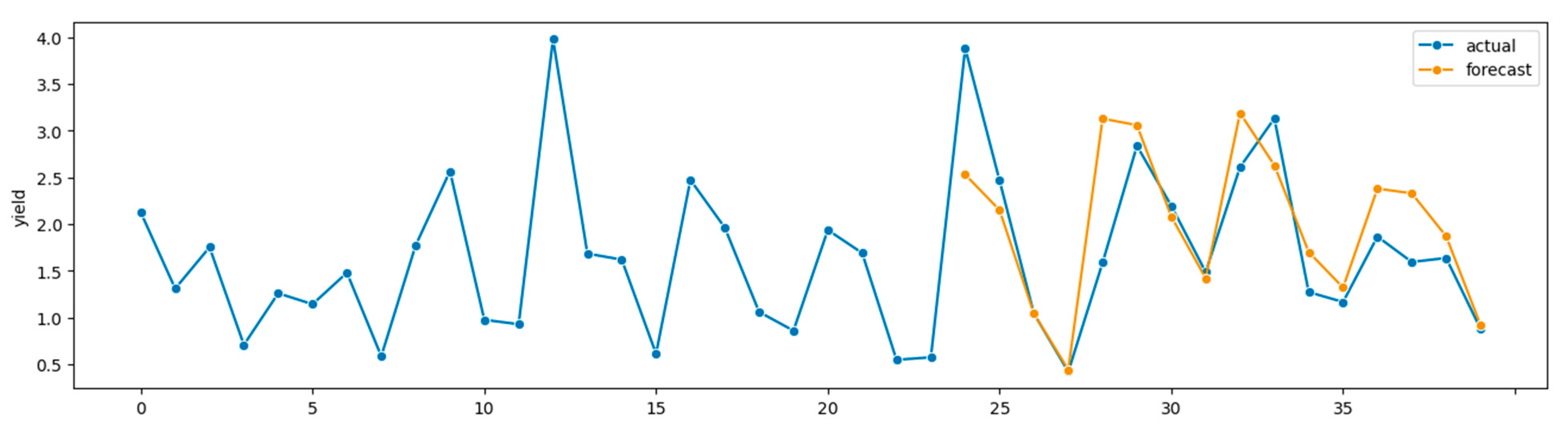Figure 2 depicts a time plot for the SVR forecaster.

Table 3. Univariate sliding window validation results. Beresford, SD. Four training windows of 6 years with each forecast of the following year, from 2008 to 2011. Top three average results in bold.

Target Year	ARIMA	SARIMA	KNN	DT	SVR	XGB	MLP	RF	LR	BRR
2008	49.47 0.62	39.05 0.88	42.22 0.99	36.62 0.99	37.04 0.74	39.38 0.79	43.18 0.99	41.22 0.93	41.01 0.99	37.46 0.99
2009	34.96 0.28	50.64 0.13	37.45 0.18	36.92 0.51	46.08 0.16	54.01 0.36	32.86 0.16	33.80 0.26	43.81 0.16	46.20 0.16
2010	29.80 0.86	14.43 0.90	27.71 0.85	59.04 0.44	25.89 0.82	71.04 0.34	26.83 0.85	39.34 0.65	23.65 0.85	22.56 0.85
2011	29.52 0.59	25.91 0.79	18.53 0.91	24.25 0.48	13.77 0.85	24.14 0.48	31.04 0.85	19.97 0.76	24.10 0.85	20.83 0.86
Average	35.94 0.59	32.51 0.68	31.48 0.73	39.21 0.48	30.70 0.64	47.14 0.49	33.48 0.71	33.58 0.65	33.14 0.71	31.76 0.71

Table 3. Univariate sliding window validation results. Beresford, SD. Four training windows of 6 years with each forecast of the following year, from 2008 to 2011. Top three average results in bold.

Target Year	ARIMA	SARIMA	KNN	DT	SVR	XGB	MLP	RF	LR	BRR
2008	49.47 0.62	39.05 0.88	42.22 0.99	36.62 0.99	37.04 0.74	39.38 0.79	43.18 0.99	41.22 0.93	41.01 0.99	37.46 0.99
2009	34.96 0.28	50.64 0.13	37.45 0.18	36.92 0.51	46.08 0.16	54.01 0.36	32.86 0.16	33.80 0.26	43.81 0.16	46.20 0.16
2010	29.80 0.86	14.43 0.90	27.71 0.85	59.04 0.44	25.89 0.82	71.04 0.34	26.83 0.85	39.34 0.65	23.65 0.85	22.56 0.85
2011	29.52 0.59	25.91 0.79	18.53 0.91	24.25 0.48	13.77 0.85	24.14 0.48	31.04 0.85	19.97 0.76	24.10 0.85	20.83 0.86
Average	35.94 0.59	32.51 0.68	31.48 0.73	39.21 0.48	30.70 0.64	47.14 0.49	33.48 0.71	33.58 0.65	33.14 0.71	31.76 0.71

Figure 2. Time plot, Table 3 SVR. Forecasts 2008–2011, true alfalfa yields 1999–2011.

Figure 2. Time plot, Table 3 SVR. Forecasts 2008–2011, true alfalfa yields 1999–2011.

Table 4 shows the results of the multivariate version of the sliding window validation experiments, where models trained on more than one feature were compared. The established model against which we compared the multivariate version of the ML-based forecasting technique is SARIMA with exogenous variables, or SARIMAX. Results from the same ML models as in the univariate version were compared. These data include precipitation, solar radiation, and temperature, and the location is Beresford, SD from 1999 to 2011, omitting 2002, 2005, and 2006 because those years did not feature four cuts. 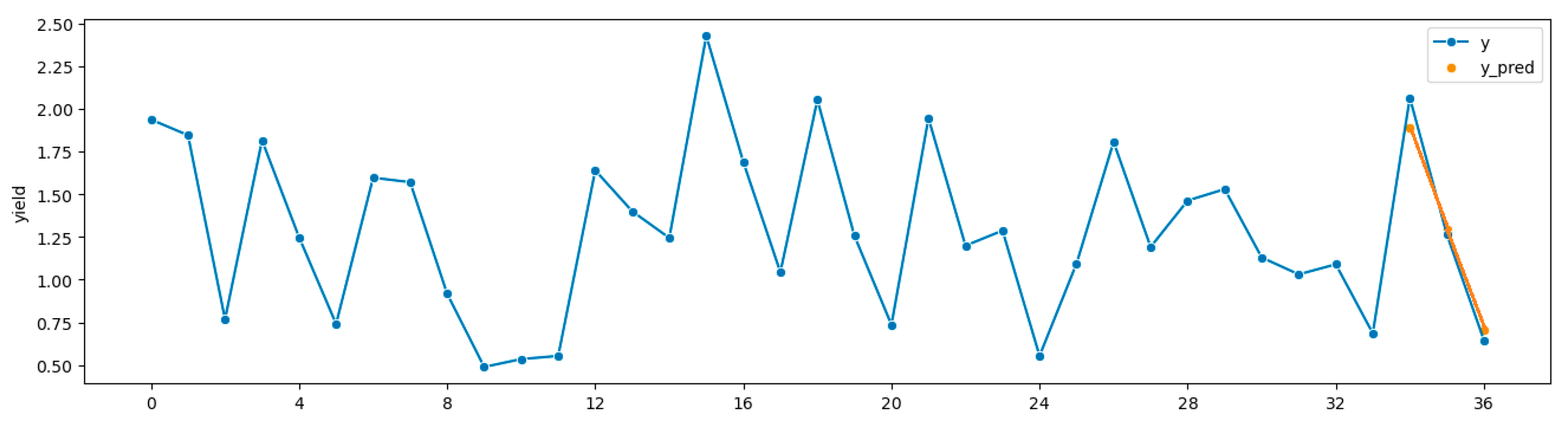Table 4 shows that the ML-based technique with stationarity results in more accurate forecasts than SARIMAX. The top row scores are sMAPE and the bottom row scores are R. RF was the top scorer in these tests, with an average sMAPE of 22.38% over all windows, and Figure 3 depicts its time plot.

Table 4. Multivariate sliding window validation results. Beresford, SD. Four training windows of 6 years with each forecast of the following year, from 2008 to 2011. Top three average results in bold.

Target Year	SARIMAX	KNN	DT	SVR	XGB	MLP	RF	LR	BRR
2008	29.33 0.97	27.47 0.96	9.08 0.99	29.61 0.99	28.24 0.98	30.90 0.99	17.23 0.98	43.79 0.84	32.13 0.99
2009	27.29 0.30	35.45 0.11	34.52 0.85	30.37 0.20	38.43 0.78	26.83 0.27	27.16 0.45	36.33 0.17	45.11 0.16
2010	29.54 0.54	16.06 0.87	48.18 0.49	21.70 0.84	36.61 0.92	18.93 0.86	23.39 0.89	31.36 0.86	22.16 0.85
2011	40.00 0.79	23.80 0.71	44.13 0.99	21.89 0.86	52.26 0.86	20.04 0.76	21.72 0.94	24.99 0.86	19.29 0.86
Average	31.54 0.65	25.70 0.66	33.98 0.83	25.89 0.72	38.89 0.89	24.18 0.72	22.38 0.82	34.12 0.68	29.67 0.72

Table 4. Multivariate sliding window validation results. Beresford, SD. Four training windows of 6 years with each forecast of the following year, from 2008 to 2011. Top three average results in bold.

Target Year	SARIMAX	KNN	DT	SVR	XGB	MLP	RF	LR	BRR
2008	29.33 0.97	27.47 0.96	9.08 0.99	29.61 0.99	28.24 0.98	30.90 0.99	17.23 0.98	43.79 0.84	32.13 0.99
2009	27.29 0.30	35.45 0.11	34.52 0.85	30.37 0.20	38.43 0.78	26.83 0.27	27.16 0.45	36.33 0.17	45.11 0.16
2010	29.54 0.54	16.06 0.87	48.18 0.49	21.70 0.84	36.61 0.92	18.93 0.86	23.39 0.89	31.36 0.86	22.16 0.85
2011	40.00 0.79	23.80 0.71	44.13 0.99	21.89 0.86	52.26 0.86	20.04 0.76	21.72 0.94	24.99 0.86	19.29 0.86
Average	31.54 0.65	25.70 0.66	33.98 0.83	25.89 0.72	38.89 0.89	24.18 0.72	22.38 0.82	34.12 0.68	29.67 0.72

Figure 3. Time plot, Table 4 RF. Forecasts 2008–2011, true alfalfa yields 1999–2011.

Figure 3. Time plot, Table 4 RF. Forecasts 2008–2011, true alfalfa yields 1999–2011.

Table 5 and Table 6 present results from ML-based forecasting with DA (ForDA), which produced the best results, like sMAPE = 9.81%. They show that ForDA beats ML-based forecasting without DA, and that SITS leads to more accurate forecasts than CTGAN or TVAE. The source data in Table 5 comes from Watertown, SD 1999 to 2011 (no 2003 due to insufficient data), and the target is Highmore, SD 1999 to 2011 (no 2000 to 2003, 2005, 2006, 2009 due to insufficient data). When data synthesis is useful due to data scarcity, these synthesis techniques will likely improve results over forecasting with TDA as previous experiments have demonstrated. Table 6 presents the results from the same technique, but with source Highmore and target Watertown, for validation. 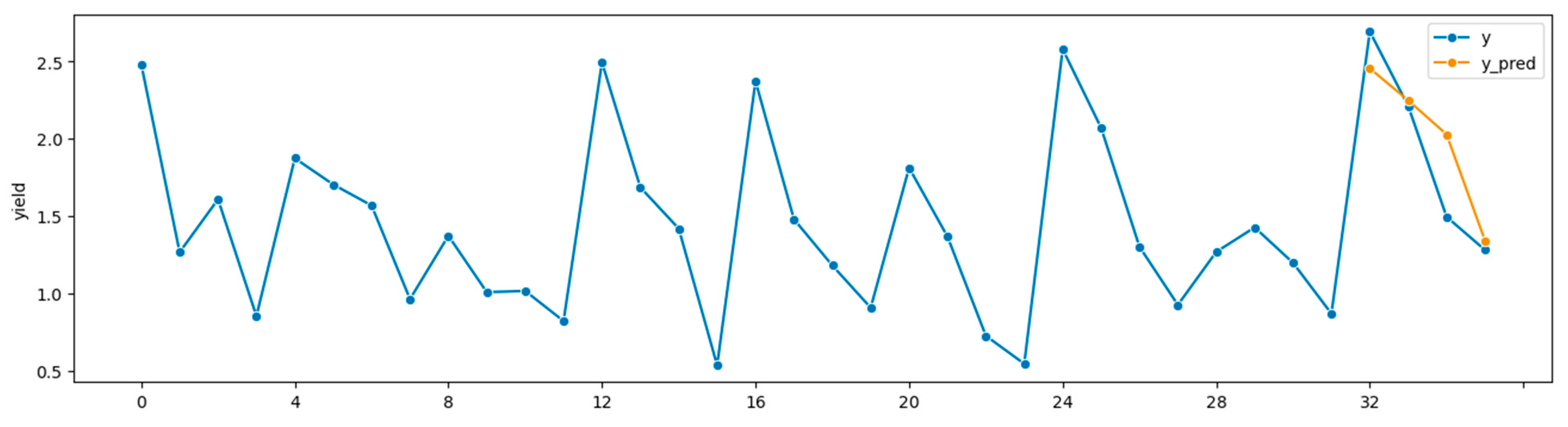Figure 4 depicts the time plot for the most successful ForDA run in Table 6. Table 7 depicts the averages of Table 5 and Table 6.

Table 5. ForDA with SITS vs. CTGAN, TVAE w/XGBoost; 20 k samples, SITS wins (bold). Source: Watertown, SD 1999 to 2011; target: Highmore, SD, 1999 to 2011.

ForDA Synth	sMAPE	R	MAE
SITS	10.22	0.87	0.21
TVAE	16.75	0.74	0.33
CTGAN	15.38	0.75	0.29

Table 5. ForDA with SITS vs. CTGAN, TVAE w/XGBoost; 20 k samples, SITS wins (bold). Source: Watertown, SD 1999 to 2011; target: Highmore, SD, 1999 to 2011.

ForDA Synth	sMAPE	R	MAE
SITS	10.22	0.87	0.21
TVAE	16.75	0.74	0.33
CTGAN	15.38	0.75	0.29

Table 6. ForDA with SITS vs. CTGAN, TVAE w/XGBoost; 20 k samples, SITS wins (bold). Source: Highmore, SD 1999 to 2011; target: Watertown, SD, 1999 to 2011.

ForDA Synth	sMAPE	R	MAE
SITS	9.81	0.94	0.14
TVAE	19.20	0.92	0.26
CTGAN	18.50	0.90	0.25

Table 6. ForDA with SITS vs. CTGAN, TVAE w/XGBoost; 20 k samples, SITS wins (bold). Source: Highmore, SD 1999 to 2011; target: Watertown, SD, 1999 to 2011.

ForDA Synth	sMAPE	R	MAE
SITS	9.81	0.94	0.14
TVAE	19.20	0.92	0.26
CTGAN	18.50	0.90	0.25

Table 7. ForDA with SITS vs. CTGAN, TVAE w/XGBoost averages; 20 k samples, SITS wins (bold). Averages of Table 5 and Table 6.

ForDA Synth	sMAPE	R	MAE
SITS	10.01	0.90	0.18
TVAE	17.98	0.83	0.30
CTGAN	16.94	0.83	0.27

Table 7. ForDA with SITS vs. CTGAN, TVAE w/XGBoost averages; 20 k samples, SITS wins (bold). Averages of Table 5 and Table 6.

ForDA Synth	sMAPE	R	MAE
SITS	10.01	0.90	0.18
TVAE	17.98	0.83	0.30
CTGAN	16.94	0.83	0.27

Figure 4. Best results from ForDA. Source: Highmore, SD 1999 to 2011; target: Watertown, SD, 1999 to 2011 sMAPE = 6.72%.

Figure 4. Best results from ForDA. Source: Highmore, SD 1999 to 2011; target: Watertown, SD, 1999 to 2011 sMAPE = 6.72%.

Table 8 shows average results from round-robin style experiments with ForDA in OH in Wooster (2011 to 2018), North Baltimore (2010 to 2018 without 2015 or 2017 due to insufficient data), and South Charleston (2010 to 2019 without 2017 due to insufficient data); each location is given a turn at being the source and another its target. These experiments showed the best results on much smaller synthesized datasets, so a sample size of 30 was settled on, as was using SITS for data synthesis, since earlier experiments suggested that it produces better results than CTGAN or TVAE for these purposes. The bottom row of Table 8 shows averages of each metric over all round-robin experiments, so it represents the average forecast accuracy in OH. Table 8 forecasts are not as striking as those where SD is the source and Beresford, SD is the target, but they are better than the ML-based forecasts without DA, and they are relatively strong forecasts overall. Also, Table 8 depicts four-point seasons. 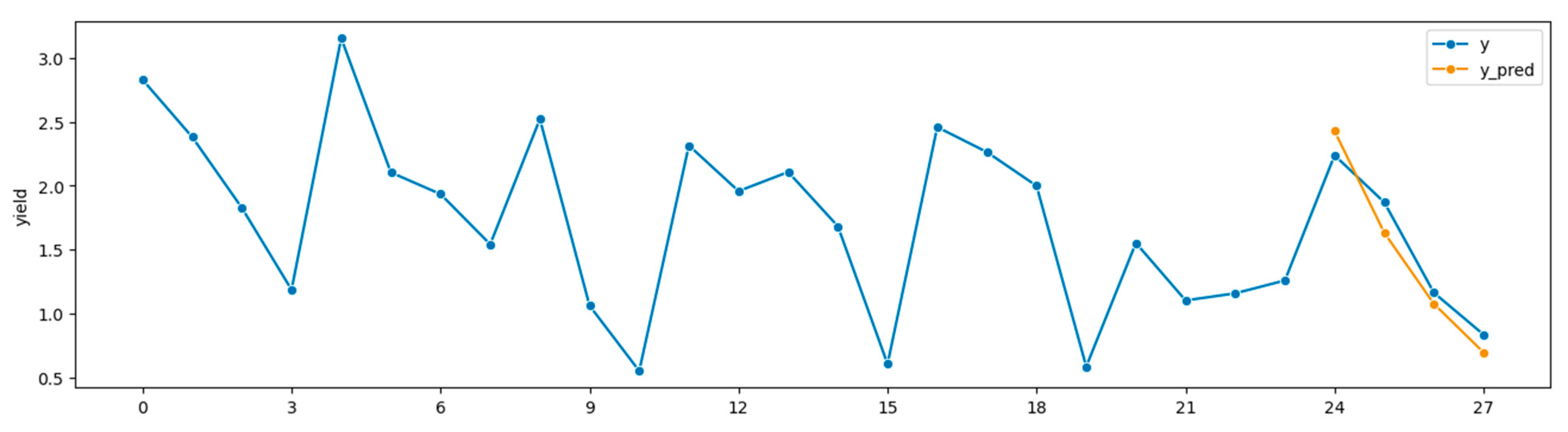Figure 5 shows the best run, which produced sMAPE = 11.45%, MAE = 0.22 tons/acre, and R = 0.88 with source Wooster and target South Charleston. Since Table 8 presents ForDA results with pretraining, all these source/target pairs use XGBoost; however, to determine whether pretraining helps, these same targets and the other seven models were also experimented with, using synthesis only and no pretraining. Those results and their corresponding time plot generally show that pretraining almost always helps, and skipping it produces mostly inferior results, with overall average sMAPE = 25.70% and R = 0.66 as shown in Table 4.

Table 8. ForDA results using SITS. Round-robin experiments in OH. Best two in bold; 2011 to 2018 in Wooster, 2010 to 2018 in North Baltimore, 2010 to 2019 in South Charleston.

Source: Target	SITS(s) Parameter	sMAPE	MAE	R
Wooster: North Baltimore	0.5	16.47	0.19	0.98
Wooster: South Charleston	1.5	16.55	0.30	0.82
North Baltimore: Wooster	1.5	26.51	0.51	0.21
North Baltimore: South Charleston	1.0	18.33	0.55	0.76
South Charleston: Wooster	2.0	22.84	0.44	0.26
South Charleston: North Baltimore	0.5	16.54	0.23	0.86
Average	-	19.54	0.37	0.65

Table 8. ForDA results using SITS. Round-robin experiments in OH. Best two in bold; 2011 to 2018 in Wooster, 2010 to 2018 in North Baltimore, 2010 to 2019 in South Charleston.

Source: Target	SITS(s) Parameter	sMAPE	MAE	R
Wooster: North Baltimore	0.5	16.47	0.19	0.98
Wooster: South Charleston	1.5	16.55	0.30	0.82
North Baltimore: Wooster	1.5	26.51	0.51	0.21
North Baltimore: South Charleston	1.0	18.33	0.55	0.76
South Charleston: Wooster	2.0	22.84	0.44	0.26
South Charleston: North Baltimore	0.5	16.54	0.23	0.86
Average	-	19.54	0.37	0.65

Figure 5. Best run in OH round-robin tests. Source: Wooster 2011 to 2018, target: South Charleston 2010 to 2019, forecasting 2019, sMAPE = 11.45%, MAE = 0.22 tons/acre, R = 0.88.

Figure 5. Best run in OH round-robin tests. Source: Wooster 2011 to 2018, target: South Charleston 2010 to 2019, forecasting 2019, sMAPE = 11.45%, MAE = 0.22 tons/acre, R = 0.88.

As Table 9 shows, LOOCV was attempted next, at the state level for sources and the local level for targets, since it is not feasible to forecast per-cut at the state level, as cut dates, weather, and number of cuts vary within the state. Three states were combined for each source and again experiments were conducted with and without synthesis, rotating among MI, OH, SD, and KY. Those results were promising in at least the case of target North Baltimore, OH, which produced a sMAPE = 15.06%, MAE = 0.16 tons/acre, and R = 0.98. SITS data synthesis clearly improved results in these tests, with an average sMAPE = 25.85%, MAE = 0.36 tons/acre, and R = 0.75 with synthesis versus sMAPE = 33.62, MAE = 0.49 tons/acre, and R = 0.65 without synthesis. Figure 6 shows a time plot from the best run of these experiments.

Table 9. ForDA LOOCV with MI (1999 to 2022), OH (2010 to 2019), SD (1999 to 2011), and KY (2012 to 2018).

Source: Target	SITS(s) param	samples	sMAPE	MAE	R
MI, OH, SD: KY	1.2	500	26.55	0.28	0.51
MI, OH, SD: KY no synth	-	-	19.82	0.19	0.71
MI, SD, KY: NB, OH	0.3	500	15.06	0.16	0.98
MI, SD, KY: NB, OH no synth	-	-	25.47	0.35	0.99
OH, SD, KY: MI	1.5	400	25.21	0.40	0.94
OH, SD, KY: MI no synth	-	-	39.39	0.56	0.88
MI, OH, KY: SD	1.2	500	36.59	0.59	0.55
MI, OH, KY: SD no synth	-	-	49.79	0.84	0.00
Average w/synth	-	-	25.85	0.36	0.75
Average no synth	-	-	33.62	0.49	0.65

Table 9. ForDA LOOCV with MI (1999 to 2022), OH (2010 to 2019), SD (1999 to 2011), and KY (2012 to 2018).

Source: Target	SITS(s) param	samples	sMAPE	MAE	R
MI, OH, SD: KY	1.2	500	26.55	0.28	0.51
MI, OH, SD: KY no synth	-	-	19.82	0.19	0.71
MI, SD, KY: NB, OH	0.3	500	15.06	0.16	0.98
MI, SD, KY: NB, OH no synth	-	-	25.47	0.35	0.99
OH, SD, KY: MI	1.5	400	25.21	0.40	0.94
OH, SD, KY: MI no synth	-	-	39.39	0.56	0.88
MI, OH, KY: SD	1.2	500	36.59	0.59	0.55
MI, OH, KY: SD no synth	-	-	49.79	0.84	0.00
Average w/synth	-	-	25.85	0.36	0.75
Average no synth	-	-	33.62	0.49	0.65

Figure 6. Source: MI, SD, KY; target: OH. SITS w/500 samples synthesized, s = 0.3, sMAPE = 11.89, MAE = 0.16, R = 0.98. Forecasting 2019.

Figure 6. Source: MI, SD, KY; target: OH. SITS w/500 samples synthesized, s = 0.3, sMAPE = 11.89, MAE = 0.16, R = 0.98. Forecasting 2019.

Our statistical analysis of the experiments presented above can be located in Table S6.

5. Future Work

To address the challenges of model robustness under extreme seasonal conditions and adaptability to climate variability, we propose the following directions for future research. These approaches aim to improve predictive reliability across abnormal years, new climate regimes, and geographically diverse environments.

5.1. Enhancing SITS with Causal and Counterfactual Reasoning

Future work should explore the integration of causal inference and counterfactual modeling into SITS. By learning causal relationships between environmental variables (e.g., precipitation, temperature) and crop yields, models can simulate “what-if” scenarios—such as droughts, heatwaves, or early-season frosts. This will help assess yield outcomes under unseen or extreme climate conditions. These methods can be evaluated using historical “abnormal year” datasets, where known anomalies (e.g., 2003 European heatwave) are held out for testing after training on climatologically normal years.

5.2. Implementing Feature-Level Domain Adaptation for Climatic Shifts

Feature-Level Domain Adaptation (FLDA) can be applied to reduce distributional shifts between historical training data and future or out-of-domain climatic conditions. For example, models trained on humid subtropical climates could be adapted to forecast in semi-arid zones experiencing increased drought frequency. FLDA aligns internal model representations between source and target climate regimes, increasing robustness without requiring complete model retraining. Evaluation should involve domain-shift testing—training on a region or period with stable climate patterns and validating on years or locations with known deviations due to climate change.

5.3. Applying Model-Agnostic Meta-Learning (MAML) for Rapid Environmental Adaptation

Model-Agnostic Meta-Learning (MAML) enables models to learn how to learn: i.e., to rapidly adapt to new tasks with minimal data. In agriculture, this may include adapting to a new crop variety, planting schedule, or a sudden climatic anomaly. Unlike traditional retraining, MAML-trained models can fine-tune quickly using only a small number of samples. In future work, we propose using MAML to simulate fast adaptation to newly observed abnormal conditions and evaluating its performance via task-based cross-validation across multiple years and crop environments.

6. Discussion

Over the course of this work, modest promise was shown with the early DA experiments, but DA was harnessed to power the final ForDA technique, which yields very promising results.

Our results generally show that data diversity presents a serious issue. When we train on one set of locations and test on another, this creates a data diversity challenge, often leading to worse results. In estimation experiments where there was disparity or diversity between training and test data, we used SITS (Scale-Invariant Tabular Synthesizer) to synthesize data based on training datasets, as it would be inappropriate and lead to overfitting to synthesize data based on test sets. The rationale for using SITS is that it is scale-invariant, making it particularly suitable for handling data from different locations with varying scales or distributions, such as environmental conditions across states like Michigan, Ohio, South Dakota, and Kentucky. The purpose is to produce more accurate estimators, and our results confirm its effectiveness, with SITS leading to R scores over 100% higher than TVAE in certain experiments (e.g., improving R from 0.36 to 0.63 when estimating past and current yields). In forecasting, we handle data diversity mainly by using the boosting mechanism in XGBoost. When the datasets for the target location are too small, we often pre-train on a different location; however, this increases diversity between training and testing data. For the purpose of producing more accurate forecasts where data are scarce, we leverage XGBoost’s ability to pre-train on a large dataset (often synthesized by SITS) and then boost training using a smaller, less divergent dataset from the target location. This approach is supported by the literature, which has shown that such methods are effective for transfer learning with XGBoost (Huber et al, 2022). Since the actual test target data remain hidden during training, this boosting step is appropriate and does not lead to overfitting. Most importantly, this approach allows us to handle data diversity when training and testing on disparate datasets while still attaining useful, relatively accurate results, as evidenced by ForDA experiments achieving sMAPE scores as low as 9.81%.

One phenomenon observed is that while models in the ARIMA family provide diminishing returns after considering too many lags in these experiments, the ML-based forecasting technique appears to only improve more as the training window widens. Another interesting observation is that ARIMA sometimes outperforms SARIMA, so trying to account for seasonality is not always helpful. On the other hand, though alfalfa yields display some seasonality, looking at the time plots reveals that the trends are not always consistent.

Until the current work, the authors have focused on estimating past and current yields as tabular data. In that problem, R and coefficient of determination (R²) scores closer to 1 are the best and usually indicate a good model that makes accurate predictions.

Readers may note that the results for forecasting the future are sometimes better than results for estimating past and current yields, which may seem surprising; however, better forecasting results are expected when they are locally trained, while the estimators are trained on non-local data. Even though ForDA pretrains on non-local source data, it ultimately trains on a small subset of data local to the target area. As the current authors showed in previous work, local training to estimate past and current yields is still arguably the most accurate, as one would expect, reporting R² scores over 0.98 (J. R. Vance).

While the results herein suggest that the proposed multivariate ML-based forecasting technique and ForDA produce more accurate forecasts than the well-established SARIMAX, this may be a little like comparing apples to oranges. The authors hypothesize that this technique wins because it is fitted to the forecast horizon’s weather features during testing to make its predictions, so it has an advantage over SARIMAX, which only looks at exogenous variables in the lags. On the other hand, the vision for the current project has always been to build a what-if tool like PYCS, where the “ifs” are the weather features in the forecast horizon, whether they are hypothetical or known, and these results indicate that the proposed techniques can forecast “what-if” with high accuracy. XGBoost often performs best with several thousand training samples, but it is not usually a top performer when the data size is very limited. On the other hand, when plenty of training data for pretraining is used and the booster function is employed, XGBoost becomes the winner. Overall, it would make this work easier if all the historical yield data was more consistent and tightly controlled, and if it went back further. While six years is enough training for this technique to beat SARIMAX, that small window might not reveal the potential of ML-based forecasting, and more data and consistency would likely help.

When ForDA was pushed to its limits, using non-local and state-level sources to forecast targets in disparate regions, it showed that ForDA is still potentially useful, but not as accurate as when sources are in-state. Therefore, and not too surprisingly, it is best to use in-state or otherwise very nearby sources and targets. While data synthesis and our SITS algorithm led to higher average accuracies than without synthesis in most experiments, synthesis did not demonstrate a clear advantage in those more challenging validation experiments. However, data synthesis continued to produce the anecdotally best models, which may be important to pay attention to, as one can save these pretrained models and reuse them in the final PYCS application, and they will likely keep and reuse those that lead to the anecdotally best results.

7. Conclusions

Through the techniques developed in this work, more accurate biomass yield forecasts are achieved than previously reported in the literature anywhere to the current authors’ knowledge. The most important contribution herein is probably ForDA, which produced forecasts with sMAPE scores as low as 9.81% versus ML-based forecasting without DA, which achieved 30.70% with the univariate and 22.38% with the multivariate approach. ForDA is the culmination of a series of ML-based techniques developed through this work, each of which incrementally improves forecast results. In the first phase, data synthesis led to improvement in predictions of past and present yields, motivating this team to continue exploring data synthesis and to creating the novel SITS. SITS improved those predictions, improving R scores from 0.36 to 0.63 over TVAE, the runner-up. After phase one, future yields were predicted in all other experiments. In phase two, ML-based models were compared against the traditional ARIMA family of forecasting models, and ML consistently forecasted alfalfa biomass yields more accurately than ARIMA. The univariate version of these experiments showed an improvement in the ML-based approach, with sMAPE scores as low as 16.94% with BRR versus 34.67% with SARIMA. The multivariate version of these experiments also showed an improvement in the ML-based approach, with sMAPE scores as low as 12.81% with KNN versus 28.08% with SARIMAX. ML-based forecasting continued to outperform the ARIMA family as experiments with sliding windows were conducted, further supporting the conclusion that ML leads to more accurate forecasts. Finally, this led to the advent of ForDA, which integrates DA into the ML-based forecasting pipeline and is based on the novel difference forecasting technique described in “Materials and Methods”. Overall, this work describes a successful journey that began with using DA to predict past and current yields, that led to the development of a novel forecasting technique and then culminated in the combination of that technique with DA, as the ForDA pipeline. Large sets of synthesized data, particularly through SITS, significantly enhance yield estimation performance as compared to using solely the original dataset as shown in Table 9.

The authors hope the science presented here will be useful and power the resulting crop yield forecasting application. This work has shown that the proposed techniques could be potentially useful in providing the underlying science that powers a what-if tool, as these multivariate forecasts are based on features, real or hypothetical, in the future. Developing a fully automated version of the PYCS what-if tool would likely require a team of dedicated software developers, but this is possible now that there is an underlying technique to support it. While the current work focuses on alfalfa yields, the final product could be used to predict any crop or any other measurable metric of crop health.