Driplines Layout Designs Comparison of Moisture Distribution in Clayey Soils, Using Soil Analysis, Calibrated Time Domain Reflectometry Sensors, and Precision Agriculture Geostatistical Imaging for Environmental Irrigation Engineering

Abstract

The present study implements novel innovative geostatistical imaging using precision agriculture (PA) under sugarbeet field conditions. Two driplines layout designs (d.l.d.) and soil water content (SWC)–irrigation treatments (A: d.l.d. = 1.00 m driplines spacing × 0.50 m emitters inline spacing; B: d.l.d. = 1.50 m driplines spacing × 0.50 m emitters inline spacing) were applied, with two subfactors of clay loam and clay soils (laboratory soil analysis) for modeling (evaluation of seven models) TDR multi-sensor network measurements. Different sensor calibration methods [method 1(M1) = according to factory; method 2 (M2) = according to Hook and Livingston] were applied for the geospatial two-dimensional (2D) imaging of accurate GIS maps of rootzone soil moisture profiles, soil apparent dielectric Ka profiles, and granular and hydraulic parameters profiles, in multiple soil layers (0–75 cm depth). The modeling results revealed that the best-fitted geostatistical model for soil apparent dielectric Ka was the Gaussian model, while spherical and exponential models were identified to be the most appropriate for kriging modelling, and spatial and temporal imaging was used for accurate profile SWC ${\theta v}_{TDR}$(m³·m⁻³) M1 and M2 maps using TDR sensors. The resulting PA profile map images depict the spatio-temporal soil water and apparent dielectric Ka variability at very high resolutions on a centimeter scale. The best geostatistical validation measures for the PA profile SWC ${\theta v}_{TDR}$ maps obtained were MPE = −0.00248 (m³·m⁻³), RMSE = 0.0395 (m³·m⁻³), MSPE = −0.0288, RMSSE = 2.5424, ASE = 0.0433, Nash–Sutcliffe model efficiency NSE = 0.6229, and MSDR = 0.9937. Based on the results, we recommend d.l.d. A and sensor calibration method 2 for the geospatial 2D imaging of PA GIS maps because these were found to be more accurate, with the lowest statistical and geostatistical errors, and the best validation measures for accurate profile SWC imaging were obtained for clay loam over clay soils. Visualizing sensors’ soil moisture results via geostatistical maps of rootzone profiles have practical implications that assist farmers and scientists in making informed, better and timely environmental irrigation engineering decisions, to save irrigation water, increase water use efficiency and crop production, optimize energy, reduce crop costs, and manage water resources sustainably.

1. Introduction

Human-induced environmental pollution leads to global warming, which, in turn, leads to wider climate change, and this is boosting evapotranspiration, thus speeding up the hydrological cycle and, moreover, climate change research, forecast shift, trends and impacts in both the average rates and the variation in hydrological factors [1]. Additionally, understanding the related processes that take place in agricultural practices, in an effort to enhance irrigation and crop sustainability and productivity (“more crop per drop”), also has an important impact in view of the upcoming climate changes and increasing human population needs [2,3,4,5]. Natural precipitation and irrigation applications provide soil moisture, and both are used for agricultural production, while the effects of climate change and land use changes are leading to soil wetness exhaustion at increasing rates.

So, in the soil–water–plant–atmosphere environment, SWC constitutes one of the many essential factors that comprise the fundamental nexus of the hydrological cycle in terrestrial ecosystems, affecting soil evaporation, land surface water runoff, infiltration, and the energy balance on the land top layer (allocation of latent and sensible heat) [5,6,7,8,9]. In addition, soil water content or soil moisture is one of the principal sources of water for plant development, defining plants’ functionality, morphology, and productivity [5,9,10,11,12].

Over the last thirty-five years, there has been a growing trend in studies addressing the interactions between climate, soil moisture, plants, and landscapes [5,10,12,13,14,15,16,17,18,19,20], but in situ datasets linking physiographical and vegetal traits to longitudinal and time-series patterns of soil moisture are scarce. Thorough insight into soil moisture status (spatially and temporally) is also vital for a broad spectrum of farming, irrigation, and soil and water resource management applications. SWC status (spatial and temporal) [10,12,20,21] in the soil layers of a plant’s rootzone can serve as an index for predicting crop yield and also plays a role in early warning and other systems (for scheduling irrigation, monitoring flooding, or drought). Soil moisture shapes the interactions that occur at the soil surface and in the atmosphere, thus affecting climate and weather [10,22,23,24,25], and is critical in terms of determining soil responsiveness to precipitation runoff, particularly where saturation and excessive runoff phenomena are significant [6,25,26]. The moisture presence in the soil is fundamental for the recirculation of soil nutrients, a prerequisite for prime production [23,27,28,29,30,31,32,33,34,35,36,37,38,39]. Evapotranspiration and its rate are directly influenced by soil moisture because evapotranspiration constitutes a key mechanism of the climate and a link to the soil water, energy, and carbon cycles, and to water supplies. As global warming and climate change are rapidly evolving due to human-induced environmental pollution, soil–water–atmosphere coupling is strengthening, enhancing the influence of soil moisture on soil surface processes and climate change [40,41,42]. Additionally, the atmospheric recirculation of summerly soil moisture will raise the air temperature and cause spatial climatic variations in Central and Eastern Europe [43].

In terms of adapting agriculture to climate change, soil moisture (SM) and precision agriculture (PA) are fundamental factors in environmental irrigation decisions and sustainable crop and soil–water resources management. Soil moisture is measured using various methods, which can be classified into two main classes: (1) direct measuring and (2) indirect measuring. In direct measurement, SM is defined as the weight variation of a soil sample prior to and after drying it. The unique direct method is the gravimetric or thermostatic weight method, which is extensively utilized for the determination of soil moisture content [44]; all other methods belong to the class of indirect methods. The gravimetric method has a test procedure that entails drying a soil sample of specified volume in an oven at 105 °C for 24 h. The soil sample’s water content is obtained by subtracting the oven-dried soil weight from the original soil weight sampled in situ in the field [45]. The soil moisture value can be stated as the percentage of water content per soil volume. This method is cost-efficient, simple, and precise, but it is laborious and time-intensive, unstructural, and hard to apply in rocky soils [46]. The application of this method constitutes a complicated task in heterogeneous land patterns [44].

The indirect measurement methods are performed via calibrations versus different measured parameters [10,47,48] that fluctuate with the soil water content. Indirect measurement methods of soil moisture estimation are classified into two main subclasses: (1) remote sensing (RS) measurements methods, and (2) ground-based measurement methods.

RS measurement methods include the satellite sensors’ usage, radar (microwaves) and passive and active sensors [49]. These methods offer an alternative instrument for materializing rapid assessments of soil properties [50]. All segments of the electromagnetic spectrum can be utilized in SM remote sensing, yet just the microwave bands are best suited for obtaining quantified measurements [50,51], as the prime physical soil characteristics that influence the measurement depend on the soil moisture content. The ground-based measurement methods are soil moisture assessment procedures, where the sensor is in close contact with the soil particles. These methods yield higher-accuracy data. The main ground-based measurement methods are neutron scattering [44,48,52,53], time-domain reflectometry (TDR) [10,20,28,53,54,55,56,57], Frequency-Domain Capacitance [48,56], Frequency-Domain Reflectometry (FDR) [5,47,48], Time-Domain Transmission (TDT) [48,54], capacitance sensor method [5,47,48], ground-penetrating radar [45,48,58,59], tensiometer, Gamma ray attenuation, gypsum block methods [5,48], and the pressure plate method [5,12,20]. Methods for measuring soil profile moisture vary, from destructive sampling, with the use of an auger or a core-tube, to non-destructive methods like neutron scattering, y-ray attenuation and capacitance readings, as well as a variety of sensors, which include heat flux-based sensors, resistance sensors, and TDR detectors placed at various soil layers and depths. Damaging destructive methods are not usually recommended because of the necessity for repeated measurements at the same field locations and the time required to handle the in situ soil samples [53]. TDR (high-accuracy method) and FDR (low-accuracy method) are fundamental methods that were developed to measure the dielectric constant of the soil’s moisture content [5,32,53,54,55,60,61,62,63]. This set of multi-sensory probes and various sensors assesses soil moisture by measuring several features of the electromagnetic signal transmitted, received and analyzed. The transmitted electromagnetic signal through the subsurface soil layers can be received, logged, processed and then subsequently evaluated to determine the bulk permittivity (or dielectric constant), which defines the time of signal propagation, its reflectivity, the shifts in frequencies, the reflect signal’s amplitude and phase, and the incoming and reflected signals [54]. The sensors, instruments and devices can be precisely calibrated, provide accurate SWC measurements at different depths of soil layers and can be recorded on any temporal interval [5], yet they only obtain point measurements, therefore making it challenging to interpret them spatially [62]. So, nowadays, but also in the years to come, there is a growing necessity for maps displaying spatio-temporal soil moisture information of various driplines layout designs to enhance spatial moisture analysis and interpretation in order to assist scientists and farmers in environmental crop–irrigation engineering decisions, water use efficiency of each d.l.d., integrated and sustainable water resource management, crop production and, also, in gaining deeper knowledge of soil–water–crop–atmosphere hydrological functions.

In this pathway, the present study implements new innovative geostatistical imaging using precision agriculture under sugarbeet field conditions with two driplines layout designs and irrigation treatments (A: d.l.d. = 1.00 m driplines spacing × 0.50 m emitters inline spacing; B: d.l.d. = 1.50 m driplines spacing × 0.50 m emitters inline spacing) applied, with two subfactors: clay loam and clay soils (via laboratory soil analysis). Modelling (evaluation of seven models) of TDR multi-sensor network measurements using different sensor calibration methods [M1=according to factory and M2=according to Hook and Livingston] was used, with geospatial two-dimensional imaging for accurate GIS mapping of rootzone soil moisture profiles, soil apparent dielectric Ka, granular and hydraulic parameter profiles, in multiple soil layers (0–75 cm depth), aiming to assist scientists and farmers in environmental irrigation decisions and sustainable crop and soil–water resources management.

2. Materials and Methods

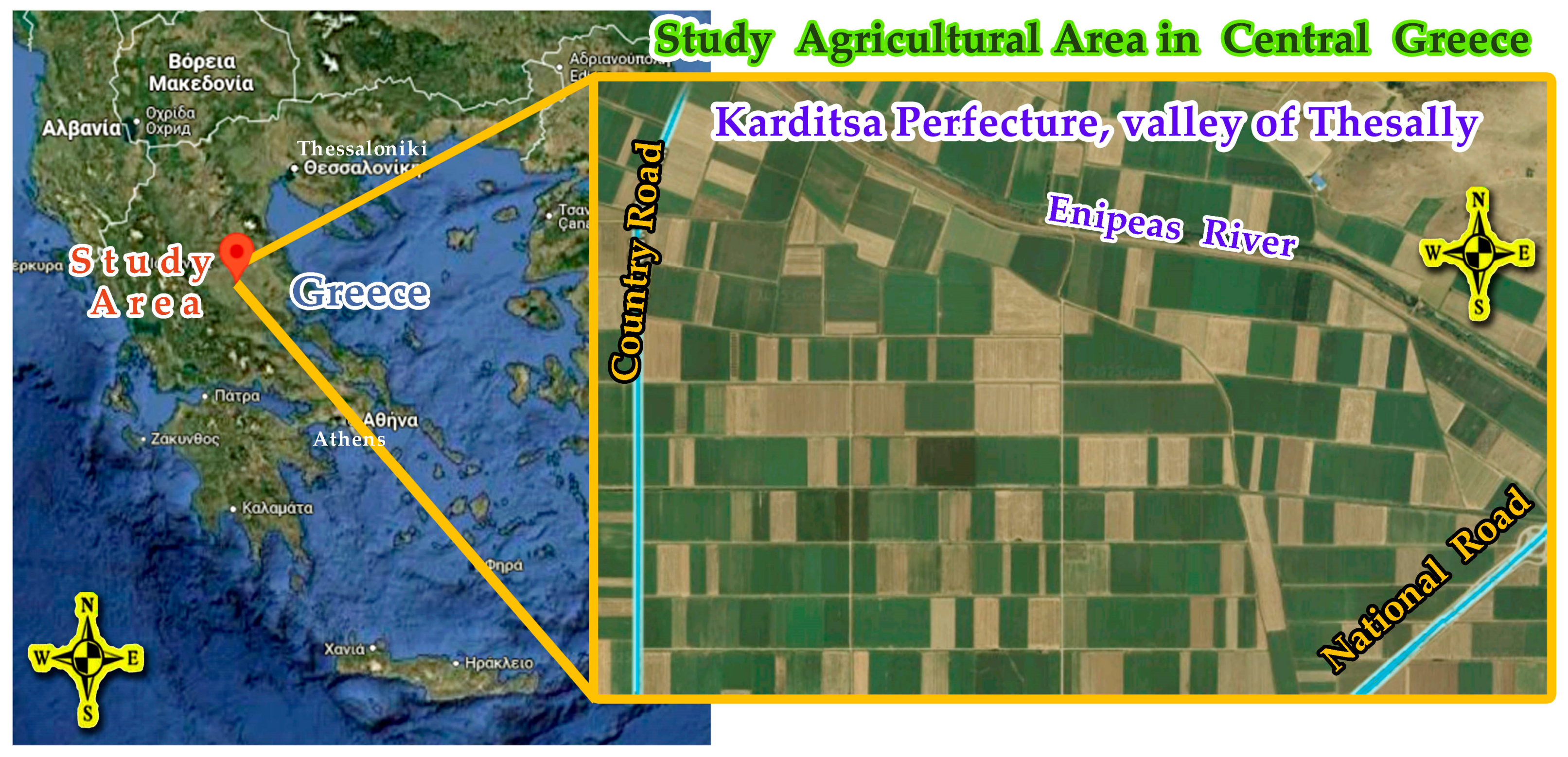
2.1. Study Area and Climatic Conditions

The experiments were conducted at sites located at Karditsa prefecture area in the valley of Thessaly (central Greece). The agricultural study area in central Greece is depicted in Figure 1. The local weather station was the source of the climatic data utilized in this study.

2.2. Sugarbeet Cultivation, Farm Machines, Farm Field Management, Fertilization, and Irrigation Pipeline System Modules and Testing

The plots of the sites were plowed in early November using a three-row reversible mounted plow. In mid-November, a spring-steel tine cultivator (having reversible attachments and wheels having floating wings) was used to till the topsoil of the plots in the experimental sites. Sugarbeet (Beta vulgaris L.) crop was sown in early April with a seed drill, spaced 0.12 m between plants in the row and 0.50 m between rows. Weed control at the plots of the experimental sites was applied by hand throughout the crop growth stages.

The pipeline network with various driplines layout designs of the irrigation system is made up of a main module with (a) a water cyclonic separator; (b) a screen-water filter; (c) several pipe fittings; (d) a main water supply polyethylene (PE) pipeline (Φ = 89 mm with nominal pressure 10.13 bar); (e) primary PE pipes (Φ = 40 mm with nominal pressure 6 bar); (f) secondary PE pipes (Φ = 25 mm with nominal pressure 6 bar); (g) polyethylene heavy wall (hw) driplines (Φ = 20 mm/4 L·h ⁻¹/0.50 m) having integral emitters with a labyrinth design that provides wide fluid pathways to enhance flushing efficiency; and (h) pressure regulators to provide accurate and equable water quantities between sites, thereby maintaining high water and nutrient concentration uniformity along the PE driplines. Prior to the use of the driplines (with the integral emitters) in field treatments, the driplines were extensively tested in the laboratory to ensure their proper functionality. The coefficient of variation (${Cv}_{em}$) of hw dripline emitters was calculated in accordance with I.S.O. standards [64].

2.3. Driplines Layout Designs, Soil Moisture Treatments and Setup Under Field Conditions in Clayey Textured Soils

The two driplines layout designs and soil moisture pattern treatments (A and B) under sugarbeet field conditions are presented in Figure 2. The designs of these two modes were based on farmers’ real applications in the study area. Some farmers in the study area consider it appropriate and use the traditional treatment A mode (d.l.d. = dripline in every other furrow), whereas other farmers consider it appropriate and use the treatment B mode (d.l.d. = dripline in every three furrows) in order to reduce the initial cost of purchasing the driplines and the installation work in their field.

Treatments A and B (Figure 2) were combinations of heavy wall (hw) driplines of 20 mm diameter with internal emitters (flow rate 4 L·h⁻¹ and inline spacing 0.50 m apart), with differing driplines layout placement spacing of every other furrow (distance = 1.00 m) or every three furrows (distance = 1.50 m). Two subfactors of clayey textured soils [clay loam (CL) and clay (C) soils] were used, i.e., [(A Treatment) = 1.00 m driplines spacing × 0.50 m integral emitters spacing under clay loam and clay soils] and (B Treatment) = 1.50 m driplines spacing × 0.50 m integral emitters spacing under clay loam and clay soils)]. The size of the trial sites was 9 m wide (across cultivation rows) and 10.5 m long (lengthwise the cultivation rows), occupying a farm area of 1134 m² (0.1134 ha). The experimental field sites were established with a completely randomized block design (CRBD) layout consisting of two treatments (A versus B) with two subfactors (CL versus C soils). Each treatment had six replications, and the total number of experimental field sites was twelve.

2.4. Sampling of Soil Layers, Laboratory Soil and Hydraulic Analysis

The manufacturer suggests two options for the TDR sensors and instrument calibration and validation. The first option suggests that they can be used with standard factory calibration without any prior validation on most soils for every site [61]. The second option suggests that they can be used with the standard factory settings or any other calibration method, and the sensors should be calibrated and validated for every soil (especially for heavy soils) and site, based on the gravimetrically determined soil water content [61]. Although the second option requires more time and labor, it is more appropriate and accurate for scientific or farmer in-field sensor applications. So, all the sensors and instruments utilized for measuring the SWC (m³·m⁻³), prior to field measurements, should be calibrated on the basis of the gravimetrically determined SWC (m³·m⁻³) using the unique direct measurement method, which is the gravimetric or thermostatic weight method [5]. This method is extensively utilized for estimating the SWC (m³·m⁻³) [44]. The present study utilized the gravimetric method as a standard method to perform the calibration procedures.

Every week for a five-week period, across the sixty (60) TDR sensors network locations, soil-core sampling was conducted to obtain a range of SWC (m³·m⁻³) values of the rootzone soil layers at depths of 0.00–0.15, 0.15–0.30, 0.30–0.45, 0.45–0.60 and 0.60–0.75 m, approximately 0.05 m apart from the TDR sensors locations. A differential global positioning system (DGPS) receiver was utilized simultaneously for soil-core sampling to identify the exact field locations of the soil-core samples. The sampling holes were meticulously re-filled with soil material taken from the same locations. Then, using the gravimetric method, the average (for each one of the five soil depths) volumetric moisture of the soil-core θvg (m³·m⁻³) was obtained in the laboratory. Additionally, the soil’s textural content [clay (Cl), sand (Sa) and silt (Si)] values were found according to standard procedures [65] and via the Bouyoucos hydrometer method [5,65]. The hydraulic properties of the soil samples (saturation (θsat), field capacity (θfc), bulk density (BD), wilting point (θwp), and soil apparent dielectric Ka) were measured in the laboratory according to standard procedures [5,65]. Soil saturation as a percentage equals the weight of water needed to saturate the pores in soil paste divided by the weight of dry soil. The θfc and θwp were measured in the laboratory using the method of a porous ceramic plate at 33.44 KPa for θfc and at 1519.88 KPa for θwp [5,65]. The soil’s saturated hydraulic conductivity (Ks) was measured for 00.00–0.15, 0.15–0.30, 0.30–0.45, 0.45–0.60 and 0.60–0.75 m soil depths using a Guelph permeameter.

2.5. Soil Moisture TDR Sensor Measurements and Calibration Models Under Field Conditions

Soil moisture measurements were taken daily and weekly applying the TDR (time-domain reflectometry) method with a network of in-field TDR sensors. TDR is a non-radioactive method that relies on directly measuring the soil’s apparent dielectric constant (Ka) and then the conversion to volumetric SWC (m³·m⁻³) [5,12,32,54,55,56,61], which has been proven to be both quick and durable, regardless of the soil characteristics, except in unusual soil situations [54,55,56,61]. The TDR was employed as it gives precise measurements with a marginal accuracy error ±1% [5,30,32,54,55,56,61]. The SWC (m³·m⁻³) on a volumetric basis, which is estimated using TDR, entails measuring the propagation velocity (or else time delay) and the attenuation of an electromagnetic step or pulse function applicable across a transmission line in the soil. The TDR device emits an electromagnetic pulse that propagates as an electromagnetic wave within the soil material via a waveguide segment (or else sensor), which acts as a transmission path. The propagation velocity (v), or time delay, and the attenuation of the electromagnetic pulse applied to the waveguide segment (or else sensor) are measured as function of time (t), and then the soil–water content (${\theta v}_{TDR}\left(p\right)$, …, ${\theta v}_{TDR}\left(n\right),$ with p = 1, 2, …, n and n = 5) of the plants’ soil–root area in n layers is calculated with the factory calibration method, or, alternatively, the user can download the time delay values from the TDR instrument and perform the soil moisture calculations using another calibration method. The propagation velocity (v) expressed in Equation (1) refers to the time it takes for an electromagnetic pulse to propagate along the entire length of the sensor (to transmission’s line termination) and then return home.

$$v={\displaystyle \frac{2L}{t}}$$

(1)

where L is the straight-line length traversed of the waveguide sensor, and t is the recorded travelling time of the electromagnetic pulse.

The time lag or time delay is the measurable parameter from the TDR device that is utilized to assess the SWC (m³·m⁻³) [63]. As the moisture in the soil increases, the time required (time delay) for the electromagnetic pulse to travel the length of the waveguide sensor will increase. Moreover, the propagation velocity is standardized with respect to the speed of light and expressed in relation to the apparent dielectric constant ($K_a$) [57], in Equation (2):

$$K_a={(c/v)}^2$$

(2)

where c is the speed of light, and $v$ is the propagation velocity of the electromagnetic pulse.

The most acceptable and used general formula for finding the SWC from the TDR recorded travelling time (or time delay) was derived by Hook and Livingston (1996) [63], where they express $v$ in terms of time intervals, as expressed as Equation (3):

$${\theta v}_{TDR}={\displaystyle \raisebox{1ex}{$\left[\left(T/T_a\right)-\left(T_s/T_a\right)\right]$}\!\left/ \!\raisebox{-1ex}{$(\sqrt{K_w}-1)$}\right.}$$

(3)

where T is the travelling time (or time delay) of TDR’s electromagnetic wave through the soil material and normalized with regard to the theoretical travelling time in the transmission line through air expressed as $T_a$; $T_s$ is the TDR’s recorded travelling time in oven-dried soil; $T_a$ is the theoretical travelling time of TDR’s electromagnetic wave in the transmission line through air; and $K_w$ is water’s dielectric constant at 20 °C.

For soil moisture measurements, a TDR instrument (model MP-917 system from ESI-Environmental Sensors INC, Sidney, BC, Canada), with a measurement data processing unit, a data logger, RG-58 connecting cables and soil moisture profile TDR sensors [61] for soil depths of 0–15, 15–30, 30–45, 45–60 and 60–75 cm [10,20,32,61], was deployed in a sensor network for measuring soil water content at multiple rootzone profile locations.

In each of the first replicate plots of the treatment sites, thirty (30) TDR sensors were carefully installed in the soil.

The TDR instrument measures T (electromagnetic pulse time delay of the transmission line).

The instrument’s factory calibration (method 1) uses, for $T_s/T_a$_, a value of 1.55 ns, which is the average value found by Hook and Livingston (1996) [63], and then the ${\theta v}_{TDR}$ of factory calibration is calculated according to Equation (4).

$${\theta v}_{TDR}={\displaystyle \raisebox{1ex}{$\left[\left(T/T_a\right)-\left(1.55\right)\right]$}\!\left/ \!\raisebox{-1ex}{$(\sqrt{K_w}-1)$}\right.}=\left[\left(T/T_a\right)-\left(1.55\right)\right]\times 0.1256$$

(4)

where T is the travelling time (or time interval, or time delay) of TDR’s electromagnetic wave through the soil material, normalized with regard to the theoretical travelling time in the transmission line through air, expressed as $T_a$; $T_a$ is the theoretical travelling time of TDR’s electromagnetic wave in the transmission line through air; and $K_w$ is water’s dielectric constant.

Additionally, in the present study, a constant value of $K_w$ was applied because the variety of temperatures found in soil profiles was within 23 to 30 °C, so the measurement errors of the apparent soil dielectrics associated with soil temperature variations within the soil profiles were negligible according to Pepin et al. (1995) [66].

Moreover, Figure 3 presents an overview methodological flowchart illustrating the experimental field, with the parameters measured in the field versus the laboratory, soil granular, hydraulic, apparent dielectrics Ka and TDR sensor moisture measurements, statistical and geostatistical modeling methodology, and validation metrics used in this study.

In addition to sensor calibration method 1 (factory or theoretical calibration), a second calibration model (method 2) was studied, as suggested by Hook and Livingston (1996) [63]. This calibration model (method 2) of ${\theta v}_{TDR}$ is presented in Equation (5):

$${\theta v}_{TDR}=\left[\left(T/T_a\right)-\left(T_s/T_a\right)\right]\times 0.1193$$

(5)

where ${\theta v}_{TDR}$ is the water content of soil derived from the TDR-recorded travelling time (or time delay) of TDR’s electromagnetic wave through the soil material; T is the travelling time (or time interval, or time delay) of TDR’s electromagnetic wave through the soil material, normalized with regard to the theoretical travelling time in the transmission line through air expressed as $T_a$; $T_a$ is the theoretical travelling time of TDR’s electromagnetic wave in the transmission line through air; and $T_s$ is the TDR’s recorded travelling time in oven-dried soil.

Moreover, the error function of ${\theta v}_{TDR}$ with respect to T is presented in Equation (6):

$${\displaystyle \raisebox{1ex}{${d\theta v}_{TDR}$}\!\left/ \!\raisebox{-1ex}{$dT$}\right.}={\displaystyle \raisebox{1ex}{$0.1193$}\!\left/ \!\raisebox{-1ex}{$T_a$}\right.}$$

(6)

Additionally, time delay data, soil moisture data and sensors’ X and Y locations of differential global positioning system (DGPS) readings for every site were entered into a digital geodatabase using PA, and the sensors’ mean volumetric SWC θv_(TDR) for each site profile was assessed by interpolating the moisture acquisitions at different depths corresponding to the different soil layers.

2.6. Statistical Analysis and Validation Metrics of Moisture Sensors’ Various Model Calibrations

Statistical analyses of soil parameters, hydraulic parameters, soil apparent dielectrics Ka, and soil moisture data descriptive statistics, Kolmogorov–Smirnov tests, parameter and map correlation, and statistical quantitative validation metrics for sensors’ various model calibrations were performed using the IBM SPSS v.27 (IBM, Armonk, NY, USA) [7,25,33,47,48,49] statistical software package.

Statistical regression of soil moisture data was used to calculate the model calibrations of sensors using methods 1 and 2. The main significant facts to consider about regression analyses are the slope (m), for determining the rate of change, and the correlation coefficient (R), a linearity index of the association between two variables [67]. Some researchers [68,69,70] expressed their concerns regarding the sole usage of R and R² in the framework of measuring the agreement between the observed and predicted values, and other studies discussed the benefits of the MAE (mean absolute error) versus RMSE (root mean square error) for estimating mean model performances [20,71,72]. Therefore, in order to validate sensors’ various model calibrations, a combination of quantitative validation metrics was used by developing algorithms in a script using IBM SPSS v.27 (IBM, Armonk, NY, USA) [7,25,33,47,48,49]. Specifically, seven statistical quantitative validation metrics were used to determine and validate which of the sensors’ various model calibration methods were best approximates to TDR sensors’ estimates of soil moisture values under field conditions, in comparison to the gravimetric laboratory measurements. The statistical quantitative validation metrics used were MAE, mean bias of absolute relative error (Pbias), RMSE, uncertainty at 95% confidence level (U₉₅), root mean squared relative error (RMSRE), relative root mean squared error (rRMSE), and the t-statistic (t-Stat).

2.7. Geostatistics Modeling for Soil Characteristics and Moisture GIS Maps Utilizing Precision Agriculture, Exploratory Data Analysis, Interpolation, Modelling and Validation Measures

The sampled, measured, analyzed laboratory soil data and sensors’ soil moisture data measurements at every site were digitized, geomapped, and modelled in a GIS environment using PA and stored in a digital geodatabase based on the samples’ attributes and field coordinates.

Ordinary Kriging (OrKr) is one of the most popular interpolation models based on Kriging methodology for predicting the spatial distribution patterns of soil attributes, soil water content, and other parameters [5,6,10,12,36]. Thus, for each experimental site, miscellaneous GIS soil parameter maps of the textural and hydraulic attributes (twelve parametric maps for each site), soil apparent dielectrics Ka maps (ten maps of Ka), and soil water content variability maps (ten maps of soil moisture ${\theta v}_{TDR}$ using sensor calibration method 1 according to factory [61], and ten maps of soil moisture ${\theta v}_{TDR}$ using sensor calibration method 2 according to Hook and Livingston (1996) [63]), were developed. The spatial fitting was implemented with the application of various geostatistical Ordinary Kriging models (seven models were evaluated) to estimate an approximate assessment of the location’s unknown value from observed field values applying exploratory geospatial and geostatistical pattern analyses, modeling and two-dimensional GIS mapping [5,20,72].

In addition, the presence of a univariate normality pattern can be graphically confirmed by boxplots and normal QQ plots and numerically using kurtosis and skewness statistical measures [73,74]. Following normalization of the data allocation, different semi-variogram models from a mathematical library of models characterizing spatial associations in geostatistical modelling were trialed and validated. To explain the spatial soil parameters and soil moisture variation at the different sites, mainly semi-variogram and interpolation scaling techniques were applied. The Kriging methodologies [5,20,75,76,77,78,79,80,81,82] are founded on the underlying assumptions that the values of the parameter characteristics (in the present study: soil’s textural and hydraulic variables, soil apparent dielectrics Ka, and soil moisture contents, of the different sites and TDR measurements) in the without-sampling zones are a good weighted average of the found values in the sampling zones of various sites. OrKr is one of the most widespread Kriging methods [5,20,72,80,81,82]. At each location X0 of each site, where no sample of the specific parameter was collected, the Z value of the soil moisture content or other soil parameters shall be calculated using Equation (7):

$$Z_{\left(X0\right)}=\sum _{s=1}^N{\mathrm{w}}_s{Z}_{\left(Xs\right)}, s=1,2,\dots ,N$$

(7)

where $Z_{\left(X0\right)}$ = the calculated value by the OrKr model of the random variables (RV) Z at the non-sampling location X0 of each site; ${\mathrm{w}}_s$ = the N weights assigned to the location $Z_{\left(Xs\right)}$ of each site.

The weights ${\mathrm{w}}_s$ shall be taken equal to unity (Equation (8)) to guarantee unbiased scaling and are calculated by the variance minimization of the estimate.

$$\sum _{s=1}^N{\mathrm{w}}_s=1.0, s=1,2,\dots ,N$$

(8)

The randomized variables $Z_{\left(X\right)}$ of each site can be divided into two components, namely the trend rate Trd_(X) and the residual rate Rsd_(X) [79], as stated in Equation (9):

$${\mathit{Z}}_{\left(\mathit{X}\right)}={\mathit{T}\mathit{r}\mathit{d}}_{\left(\mathit{X}\right)}+{\mathit{R}\mathit{s}\mathit{d}}_{\left(\mathit{X}\right)}$$

(9)

OrKr presumes the stationarity of the data average and assumes that the trend component Trd_(X) is a stable but unspecified value. Non-stationary limitations are derived by constraining the stationarity to a localized spatial neighborhood and rolling it to the entire study area of each site. The residual component Rsd_(X) is modeled as a stable randomized variable with zero average and undergoes the endogenous stationarity hypothesis; thus, its spatial dependence is determined by the semi-variance ${\gamma }_{\left(h\right)}$ under the assumption of a stationary average Trd_(X) [72]. The semi-variance ${\gamma }_{\left(h\right)}$ is an unbiased estimator mathematical function that is 0.5 of the mean squared difference between sample parametric paired data values [77,82], as defined in Equation (10):

$${\gamma }_{\left(h\right)}={\displaystyle \frac{1}{2N\left(h\right)}}\sum _{j=1}^{N\left(h\right)}\left[{Z\left(x_j\right)-Z\left(x_j+h\right)}^2\right] , j=1,2,\dots ,N(h)$$

(10)

where ${\gamma }_{\left(h\right)}$ = semi-variance at a given distance h; h = a given distance applied using a specific tolerance; $N\left(h\right)$ = number of sample parametric pairs at a given distance h from each other; $Z\left(x_j\right) and Z\left(x_j+h\right)$ are sample parametric values of two points $\left[\right(x_j) and \left(x_j+h\right)]$ separated by distance h.

To investigate and evaluate the spatial variability of soil and hydraulic properties across sites, OrKr semi-variograms were calculated for each soil, as well as for the soil water content measured by the TDR sensors each week during the measurement period. The twenty-four final precision agriculture GIS site maps of soil’s textural and hydraulic parameter datasets, the ten soil apparent dielectrics Ka maps, as well as the twenty PA SWC ${\theta v}_{TDR}$ GIS site maps (ten maps of SWC ${\theta v}_{TDR}$ using method 1 of sensor calibration according to factory [61], and ten maps of SWC ${\theta v}_{TDR}$ using method 2 of sensor calibration according to Hook and Livingston (1996) [63]) were modeled and generated. The best-fitted semi-variogram models were utilized to describe the spatial patterns of numerous soil and hydraulic attributes, soil apparent dielectrics Ka and soil’s water content measured using TDR sensors for each soil property dataset at each site.

For every soil property dataset at each site, seven semi-variogram models were trialed. These semi-variogram models were Gaussian, exponential, stable, pentaspherical, tetraspherical, spherical and circular, reflecting the different variability spatially induced by nature of the soil property, which is related to the prevailing environmental conditions of each site. The different model efficiencies obtained via Ordinary Kriging methodology were validated by cross-validation, computation of statistical measures (forecast model errors) and model performance testing with training and validation datasets. In addition, the reliability of the results of geostatistical models involves validation measures with statistical analyses of residual errors, gaps between predicted and observed values, and categorization of the prediction between over- and underestimates, as discussed in previous studies [7,13,70,71,72,73,74,75,76,83,84,85,86]. These validation statistical model metrics are Nash–Sutcliffe Model efficiency (En-s or NSE) [5,87,88,89], mean prediction error (MPE), RMSE, relative root mean square error (RRMSE) as a metric of prediction accuracy between parameters with different formats, mean standardized prediction error (MSPE) as a metric of unbiased forecasts, root mean square standardized error (RMSSE) as a benchmark for a proper assessment of the forecast variability [13,70,71,72,73,74,75,76], average standard error (ASE) as a measure of the accuracy of the true population mean [7], and mean squared deviation ratio (MSDR) as a measure of each model’s total error (relative to spread in predicted data) [5,12,81]. The MSPE and RMSSE measures are applied to assess unbiasedness and uncertainty, respectively. The MPE and MSPE should converge to zero for an optimal prediction; Nash–Sutcliffe Model efficiency, RMSSE and MSDR with larger values close to 1.0 are better; a smaller RMSE yields a better optimal prediction; a smaller RRMSE yields greater accuracy; a smaller ASE signifies greater model accuracy; and an MSDR close to 1.0 indicates a model’s lower total error (relative to spread in predicted data) and a better model. Moreover, at the validation phase, for each model, a performance simulation with 1000 iterations was executed for each soil property and the TDR’s soil moisture dataset to obtain greater possible fitting of the training (50% of the full dataset) and validation (50% of the full dataset) data for each site, taking into consideration the average fit, the best RMSE and the R-square.

3. Results and Discussion

3.1. Climate of Experimental Sites and of Emitters’ Testing

The study region is characterized by a typically Mediterranean climate [5,6,90] with a cool winter climate, a warm summer with frequent periods of hot air temperatures with low rainfall in spring and summer. The region’s mean annual rainfall is 724.77 mm and also presents a mean monthly rainfall of 60.40 mm (values vary between 22.16 and 103.10 mm), a mean monthly air temperature of 15.74 °C (values vary between 4.68 and 26.12 °C), a mean monthly maximum air temperature of 28.33 °C (values vary between 16.49 and 38.28 °C), a mean monthly minimum air temperature of 5.01 °C (values vary between −6.12 and 15.66 °C), a mean monthly maximum relative humidity of 88.18% (values vary between 83.33 and 91.21%) and a mean monthly minimum relative humidity of 49.05% (values vary between 36.35 and 64.75%). Over the last 10-year period, the mean daily maximum air temperature reached 28.35 °C (values vary between 9.30 and 42.70 °C), and the mean daily minimum air temperature reached 4.99 °C (values vary between −17.00 °C and 16.50 °C). The amount of rainfall and its temporal spread over the four crop growth stages (April to October) do not fully satisfy the crop’s water requirements for rainfed cultivation and proper growth, so irrigation and sufficient soil moisture in the rootzone are a necessity for achieving high yields [7,25,33,59,82]. Regarding the performance of the integrated emitters in the heavy wall driplines of the drip irrigation system, the laboratory results showed that emitters had a flow rate of 4 L·h⁻¹ at a test pressure of 122 kPa, in accordance with I.S.O. standards [64], ensuring high water uniformity and nutrient distribution along the heavy wall driplines.

3.2. Soil’s Granular and Hydraulic Analyses

Soil texture and hydraulic parameters, which affect nearly every aspect of soil management and especially soil moisture and irrigation decisions [5], were classified as clayey textured soils in two classes as clay loam (CL) and clay (C) soils [5,91,92,93]. The soil attributes of the trial sites differed widely, and a closer examination of the outcomes of the soil’s granular and hydraulic analyses in the laboratory showed that the sites’ soil was appropriate for the growth of sugarbeet [5,90,93]. The soil laboratory analyses results showed that the clay (size: <0.002 mm) (%), silt (size: 0.002–0.02 mm) (%), saturation θsat (% vol.), and field capacity θfc (% vol.) of both textures (clay loam and clay soils) exhibited high mean values (≥27.66), while the remaining soil characteristics showed low mean values (<27.66) for both soil textures. It should be noted that the outcomes for θfc and θwp resulting from the hydraulic analysis of the soil are in accordance with the typical ranges reported by Allen et al. (1998) [92].

The soil hydraulic conductivity is valuable for calculating the drainage of the soil’s root horizons, irrigation quantities, water runoff from rainfall, and deep drainage, which are factors that contribute to salinity [5,93,94]. The saturated hydraulic conductivity Ks results of the sites’ soils were classified as “moderate” for clay loam soils and as “very slow” for clay soils, which showed similar Ks values to those reported by Geeves et al., 2007 [95].

The soil erodibility (Kfactor) mean site values of clay loam soils (Kfactor = 0.0372 (±0.00047) Mg·ha·h·ha⁻¹·MJ⁻¹·mm⁻¹) and of clay soils (Kfactor = 0.0420 (±0.00076) Mg·ha·h·ha⁻¹·MJ⁻¹·mm⁻¹) were categorized as moderate and as high Kfactor, respectively, based on the universal soil loss equation (USLE) [96,97]. It is remarked that the soil erodibility results were within the normal limits given by Rosewell and Loch (2002) [98]. In addition, soil erodibility is an important factor that is compensated by soil moisture, because when there is increased moisture in the soil, soil erodibility and residue decomposition increase.

The StDs of the considered attributes vary widely (

Table 1. Descriptive statistics of soil granular and hydraulic characteristics for various soil textures.

SN	Parameter	Range	Minimum	Maximum	Mean	StD *	Variance	CV (%)	CV Category
		Clay Loam (CL) Soils of Sites A and B
1	Clay (<0.002 mm) (%)	10.32	29.66	39.98	34.00	2.67	7.15	7.87	Low
2	Gravel (% wt)	0.24	0.01	0.25	0.09	0.05	0.00	54.36	High
3	Sand pr (0.2–2 mm) (%)	3.91	10.32	14.22	12.00	0.97	0.94	8.07	Low
4	Silt (0.002–0.02 mm) (%)	8.71	36.46	45.17	39.94	2.06	4.26	5.17	Low
5	Soil erodibility [Kfactor] (Mg·ha·h·ha−1·MJ−1·mm−1)	0.01	0.03	0.04	0.04	0.00	0.00	8.99	Low
6	Vfs sand (0.02–0.2 mm) (%)	3.80	12.08	15.89	14.07	0.84	0.71	5.98	Low
7	Bulk density (g·cm−3)	0.22	1.24	1.46	1.34	0.05	0.00	3.48	Low
8	Field capacity θfc (% vol.)	3.61	37.25	40.86	38.87	0.84	0.71	2.17	Low
9	Plant available water (m3·m−3)	0.03	0.12	0.15	0.14	0.01	0.00	4.48	Low
10	Saturation θsat (% vol.)	6.69	47.37	54.06	51.75	1.63	2.64	3.14	Low
11	Sat. hydraulic conductivity Ks (10−3·cm·s−1)	17.30	4.37	21.67	14.15	3.85	14.81	27.19	Moderate
12	Wilting point θwp (% vol.)	5.01	22.34	27.36	24.38	1.18	1.39	4.83	Low
	Parameter	Clay (C) soils of sites A and B
13	Clay (<0.002 mm) (%)	7.32	41.63	48.94	44.36	2.75	7.56	6.20	Low
14	Gravel (% wt)	0.07	0.01	0.08	0.05	0.03	0.00	58.86	High
15	Sand pr (0.2–2 mm) (%)	1.64	7.65	9.30	8.45	0.69	0.48	8.20	Low
16	Silt (0.002–0.02 mm) (%)	5.54	32.67	38.21	35.18	1.76	3.08	4.99	Low
17	Soil erodibility [Kfactor] (Mg·ha·h·ha−1·MJ−1·mm−1)	0.01	0.04	0.04	0.04	0.00	0.00	5.75	Low
18	Vfs sand (0.02–0.2 mm) (%)	2.57	10.74	13.31	12.01	1.20	1.45	10.02	Low
19	Bulk density (g·cm−3)	0.04	1.68	1.72	1.70	0.01	0.00	0.73	Low
20	Field capacity θfc (% vol.)	1.53	33.45	34.98	33.93	0.55	0.30	1.61	Low
21	Plant available water (m3·m−3)	0.01	0.11	0.12	0.12	0.00	0.00	3.68	Low
22	Saturation θsat (% vol.)	3.06	35.64	38.71	37.24	0.92	0.84	2.47	Low
23	Sat. hydraulic conductivity Ks (10−3·cm·s−1)	0.83	0.08	0.91	0.33	0.26	0.07	78.83	High
24	Wilting point θwp (% vol.)	2.72	20.74	23.46	21.97	0.90	0.80	4.07	Low

* StD = standard deviation of the data, (N = 60 for each parameter).

). A small standard deviation indicates that the data values are close to the mean value, whereas a big StD indicates that the data values are scattered over a wide spread. The highest StD found was 3.848 for saturated hydraulic conductivity Ks in clay loam soils and 2.750 for clay content (size: <0.002 mm) in clay soils. The statistic coefficient of variation (CV) represents the variation in a soil attribute and is grouped into three main categories [20,99]: (a) low category (CV < 15%), (b) moderate category (CV = 15–35%), and (c) high category (CV > 35%). The output of the statistical analysis (as descriptive statistics) is presented in Table 1.

The statistic coefficient of variation (CV) represents the variation in a soil attribute and is grouped into three main categories [20,99]: (a) low category (CV < 15%), (b) moderate category (CV = 15–35%), and (c) high category (CV > 35%). The resulting CV percentages revealed that data variation ranking yielded ten of the twelve tested soil attributes of clay loam soils as low CV and also ten of the twelve tested soil attributes of clay soils as low CV. High CVs were found for gravel (% wt) data up to 54.355% for CL soils and 58.859% for C soils. The CVs of saturated hydraulic conductivity Ks (10⁻³·cm·s⁻¹) were found to be 27.188% for CL soils and 78.834% for C soils. Both coefficients of variation of gravel (% wt) showed variability ranked in the high category (CV > 35%) in both CL and C soils. The variation coefficients of saturation hydraulic conductivity Ks (10⁻³·cm·s⁻¹) ranked as high and moderate for C and CL soils, respectively. Environmental and/or anthropogenic influences, such as agricultural management, soil composition, soil chemical, granular and hydraulic properties and processes, and the impacts of the changing climate, could possibly contribute to their high variance.

3.3. Exploratory Data Analysis and Precision Agriculture Geostatistical Modelling of Soil’s Granular and Hydraulic Parameters

An exploratory data analysis was performed prior to geostatistical analysis and modeling. Two significant statistical measures of the tested soil characteristics in the experimental plots are skewness and kurtosis [80,81,100]. Skewness statistics were positively altered (right-tailed skewness) from 0.042 to 1.486 for the following soil properties (in ascending order): soil erodibility [Kfactor] (Mg·ha·h·ha⁻¹·MJ⁻¹·mm⁻¹), gravel (% wt), clay (%), and bulk density (g·cm⁻³). Conversely, the skewness changed negatively (left-tailed skewness) from −1.596 to −0.074 for the next soil properties (in ascending order): saturation θsat (% vol.), field capacity θfc (% vol.), plant available water PAW (m³·m⁻³), Vfs sand (%), sat. hydraulic conductivity Ks (10⁻³·cm·s⁻¹), sand pr (%), silt (%), and wilting point θwp (% vol.), (%). The results for the two statistics indicated that eight out of twelve parametric datasets (soil, granular, and hydraulic characteristics) required transformation to verify that the assumption of variance equality for data values is satisfactory and that their data points are normally distributed [5,101]. Moreover, the results of Kolmogorov–Smirnov tests showed that these soil property datasets had a non-normal data distribution [72,102,103,104,105]. Therefore, in these datasets, box–cox and logarithmic transformations were applied [72,101,102]. The transformed parameters with logarithmic transformation were BD (g·cm⁻³), θfc (% vol.), PAW (m³·m⁻³), clay (%), gravel (% wt) and Vfs sand (%). The transformed parameters with box–cox transformation were θsat (% vol.) and Ks (10⁻³·cm·s⁻¹).

In agro-ecosystems, the spatial diversity of soil attributes can be estimated by using geostatistical analysis and modelling interpolation [5,12,20,30,92,101,103]. Ordinary Kriging (OrKr) interpolation proved to be the most widely implemented interpolation model for estimating the spatial layout of soil, water, and crop attribute diversity [5,20,28,30,101,105,106,107,108,109,110]. The selection of the OrKr model to be employed is driven by the properties and statistical data metrics and the favored spatial model [20]. The results of the granular analysis for all soils at all sites obtained the following mean values: clay (<0.002 mm) = 35.723 (±0.609)%, gravel = 0.082 (±0.006)% wt, sand pr (0.2–2 mm) = 11.404 (±0.209)%, silt (0.002–0.02 mm) = 39.144 (±0.347)%, very fine sand (0.02–0.2 mm) = 13.729 (±0.153)%, and Kfactor = 0.0380 (±0.0005) Mg·ha·h·ha⁻¹·MJ⁻¹·mm⁻¹. Therefore, the accurate estimation of these soil variables depends on the existence of spatial dependencies and correlations between the sample observed data at each site, as determined by the semi-variogram [104]. The created twelve PA spatial variability maps for 0–75 cm depth of soil “Granular Group” (Figure 4a–f) revealed that clay (%) and silt (%) maps were alike in terms of spatially variation patterns. Such spatially consistent variation is due to the fact that these soil characteristics are interrelated, and, additionally, they were found to have a correlation coefficient (r_cc) [72,73,74] of very strong negative correlation (r_cc = −0.909).

In Figure 4a, the clay content (%) map patterns were also found to have strong negative correlation r_cc = −0.707 (p = 0.01 (two-tailed)) with sand pr (size: 0.2–2 mm) content (%) map patterns and with very fine sand (size: 0.02–0.2 mm) content (%) map patterns having r_cc = −0.675. PA soil maps generated for the “Granular Group” features revealed that the maps of the clay fraction (size: <0.002 mm) (Figure 4a) and silt fraction (size: 0.002–0.02 mm) (Figure 4c) were very alike in terms of spatial variation patterns, with very strong negative correlations among all sites and treatments. This consistent spatial variation is due to the fact that these two soil characteristics are closely related in nature and showed very strong negative correlation r_cc = −0.909 (p = 0.01 (two-tailed)). Furthermore, the spatial variability in sand pr and Vf sand maps were in contrast to the variability in the clay fraction maps (size: <0.002 mm) given their reversed nature, with an enhancement in one lowering the content of the other. For the sand pr (%) map patterns (Figure 4b), except the outcome that shows strong negative correlation r_cc = −0.707 with the clay (%) maps, they present moderate positive correlations with silt (%), Vf sand (%) and gravel (%) maps.

The silt (size: 0.002–0.02 mm) (%) map patterns’ (Figure 4c) correlation, except the outcome that presents very strong negative correlation r_cc = −0.909 only with the clay (size: <0.002 mm) (%) map patterns, presents moderate positive correlation with sand pr (size: 0.2–2 mm) (%) and Vf sand (size: 0.02–0.2 mm) (%) maps. A correlation matrix of soil “Ggranular Ggroup” parametric maps is presented in

Table 2. Correlation matrix of granular group parameter maps.

Correlations of Granular Group Parameters Maps	Clay (<0.002 mm) (%)	Gravel (% wt)	Sand pr (0.2–2 mm) (%)	Silt (0.002–0.02 mm) (%)	Kfactor (Mg·ha·h·ha−1·MJ−1·mm−1)	Vfs Sand (0.02–0.2 mm) (%)
Clay (<0.002 mm) (%)	1
Gravel (% wt)	−0.100	1
Sand pr (0.2–2 mm) (%)	−0.707 **	0.440 **	1
Silt (0.002–0.02 mm) (%)	−0.909 **	0.114	0.580 **	1
Soil erodibility [Kfactor] (Mg·ha·h·ha−1·MJ−1·mm−1)	−0.169	−0.479 **	−0.237	0.038	1
Vfs sand (0.02–0.2 mm) (%)	−0.675 **	−0.425 **	0.543 **	0.492 **	0.228	1

** Correlation is significant at 0.01 level (2-tailed).

.

As discussed previously, the four fractions (clay, silt, sand pr and Vf sand) of soil particles are a fixed number (100%), and they are inversely related to one another, except for sand pr with very fine sand and silt. Therefore, it was an expected result that maps of silt (%), sand pr (%), and Vf sand (%) were found to be very strongly, strongly and strongly negatively correlated with clay (size: <0.002 mm) (%) maps (Figure 4a).

The hydraulic attribute analysis of the sites’ soils obtained the following mean values: θfc = 38.044 (±0.261)% vol., wilting point θwp = 23.976 (±0.187)% vol., saturation θsat = 49.331 (±0.731)% vol., PAW = 0.1346 (±0.0013) m³·m⁻³ and bulk specific gravity or bulk density BD = 1.400 (±0.018) g·cm⁻³. A correlation matrix of the soil “Hhydraulic Ggroup” parametric maps is presented in

Table 3. Correlation matrix of hydraulic group parameter maps.

Correlations of Hydraulic Group Parameters Maps	Bulk Density (g·cm−3)	Field Capacity θfc (% vol.)	Plant Available Water (m3·m−3)	Saturation θsat (% vol.)	Ks (10−3·cm·s−1)	Wilting Point θwp (% vol.)
Bulk density (g·cm−3)	1
Field capacity θfc (% vol.)	−0.680 **	1
Plant available water (m3·m−3)	−0.770 **	0.243	1
Saturation θsat (% vol.)	−0.718 **	0.787 **	0.484 **	1
Sat. Hydraulic conductivity Ks (10−3·cm·s−1)	−0.681 **	0.360 **	0.790 **	0.775 **	1
Wilting point θwp (% vol.)	−0.485 **	0.916 **	0.020	0.547 **	0.082	1

** Correlation is significant at 0.01 level (2-tailed).

.

The generated twelve PA variability maps of soil “Hhydraulic Ggroup” parameters (Figure 5a–f) revealed that θfc (% vol.) maps and θwp (% vol.) maps were alike in their spatial variation patterns. The generated maps of field capacity θfc (Figure 5b) depict highly congruent spatial variation patterns with wilting point θwp (Figure 5c) maps (r_cc = 0.916). The field capacity θfc (% vol.) map patterns (Figure 5b) at the p = 0.01 level (two-tailed), present significant very strong positive correlation with wilting point θwp (% vol.) map patterns (Figure 5c).

Also θfc (% vol.) map presents significant strong positive correlation r_cc = 0.787 with saturation θsat (% vol.) and strong negative correlation r_cc = −0.680 with soil’s bulk density BD (g·cm⁻³) maps (Table 3).

The bulk density BD (g·cm⁻³) map patterns (Figure 5d) are strongly negatively correlated with the other hydraulic parameters maps [field capacity θfc (% vol.), plant available water PAW (m³·m⁻³), saturation θsat (% vol.), and saturated hydraulic conductivity Ks (10⁻³·cm·s⁻¹)], except the wilting point θwp (% vol.) maps, which present a moderate negative correlation. The wilting point θwp (% vol.) map patterns (Figure 5c), except the outcome that presents significant strong positive correlation r_cc = 0.916 with field capacity θfc (% vol.) maps (Figure 5b), present moderate positive and negative correlations with saturation θsat (% vol.) maps (Figure 5a) and BD (g·cm⁻³) maps (Figure 5d), respectively.

The developed maps of PAW (m³·m⁻³) (Figure 5f) show a congruent strong positive variation pattern with the Ks (10⁻³·cm·s⁻¹) maps in Figure 5e (r_cc = 0.790) and a strong negative pattern with soil’s BD (g·cm⁻³) maps in Figure 5d (r_cc = −0.770), whereas they presented moderate positive correlation patterns with saturation θsat (% vol.) maps (Figure 5a).

The saturation θsat (% vol.) map patterns (Figure 5a) at the p = 0.01 level (two-tailed), except the outcome that presents significant strong positive correlation r_cc = 0.787 with field capacity θfc (% vol.) maps (Figure 5b) and saturated hydraulic conductivity Ks (10⁻³·cm·s⁻¹) maps (Figure 5e), also present strong but negative correlation with bulk density BD (g·cm⁻³) map patterns (Figure 5d).

The generated twenty-four precision agriculture rootzone profile site maps of soil’s hydraulic and textural parameter datasets visualize the spatial variation in the examined soil variables and could be potentially applied to site-specific TDR sensor measurements and on management zones (MZs) in precision agriculture.

Soil’s hydraulic and textural parameter PA rootzone profile site maps offer precise spatial information of crop’s rootzone textural and hydraulic environmental conditions and of important hydraulic limits and parameters. The role of soil particle-size distribution is dominant in controlling soil moisture in the rootzone, regardless of the soil moisture conditions. This study’s findings will be helpful to farmers and could be applied in precision agriculture in order to choose appropriate irrigation technologies or practices and in order to decide and plan accurate crop rootzone irrigation and fertigation management, to save irrigation water, increase water use efficiency and crop production, optimize energy, reduce crop costs and manage water resources sustainably.

3.4. Results and Discussion of TDR Sensor Measurements of Rootzone Soil Water Content (${\theta v}_{TDR}$) Under Sugarbeet Field Conditions Using Various Methods of TDR Sensor Calibration

The gravimetric θvg in clay loam soils varied from 0.1288 to 0.4018 m³·m⁻³ (mean CL soils θvg = 0.2604 (±0.0039) m³·m⁻³ in combined treatments A and B of experimental sites), and the gravimetric θvg in clay soils varied from 0.2226 to 0.3485 m³·m⁻³ (mean C soils θvg = 0.2848 (±0.0041) m³·m⁻³ in combined treatments A and B of experimental sites).

The coefficient of variation for the gravimetric soil-core water content θvg (m³·m⁻³) was classified as moderate CV for clay loam soils and also for all soils (combined data of CL and C soils), but for clay soils, it was classified as low CV in all experimental sites.

The TDR sensor field measurements of SWC ${\theta v}_{TDR}$ (m³·m⁻³) based on method 1 of sensor calibration [61] in clay loam soils varied from 0.1660 to 0.4650 m³·m⁻³ (mean CL soils ${\theta v}_{TDR }$ = 0.3155 (±0.0046) m³·m⁻³ in combined treatments A and B of experimental sites), and the ${\theta v}_{TDR}$ (m³·m⁻³) using method 1 of sensor calibration [61] in clay soils varied from 0.2700 to 0.3884 m³·m⁻³ (mean C soils ${\theta v}_{TDR}$ = 0.3480 (±0.0047) m³·m⁻³ in combined treatments A and B of experimental sites).

The statistical analyses [73] of laboratory outcomes for the gravimetric soil-core water content θvg (m³·m⁻³) and TDR sensor field measurements of soil moisture ${\theta v}_{TDR}$ (m³·m⁻³) M1 and M2 based on method M1 [61] and M2 [63] of sensor calibration, as descriptive statistics results, are presented in

Table 4. Results of gravimetric soil-core water content θvg (m³·m⁻³), and TDR sensor field measurement outcomes of SWC ${\theta v}_{TDR}$ (m³·m⁻³) M1 and M2, with sensor calibration methods 1 and 2, in sites A and B.

SN	Treatment (Tr.)	N	Range	Minimum	Maximum	Mean	StD	Variance	CV (%)	CV (Category)
Soil-Cores water content θvg (m3·m−3) results using gravimetric method [5,65]
1	Tr. A-All soils	150	0.2730	0.1288	0.4018	0.2586	0.0602	0.0036	23.2680	Moderate
2	Tr. A-Clay Loam soils	125	0.2730	0.1288	0.4018	0.2551	0.0639	0.0041	25.0335	Moderate
3	Tr. A-Clay soils	25	0.1258	0.2226	0.3485	0.2762	0.0320	0.0010	11.5794	Low
4	Tr. B-All soils	150	0.2556	0.1323	0.3879	0.2703	0.0569	0.0032	21.0348	Moderate
5	Tr. B-Clay Loam soils	125	0.2556	0.1323	0.3879	0.2656	0.0604	0.0037	22.7529	Moderate
6	Tr. B-Clay soils	25	0.0925	0.2406	0.3331	0.2934	0.0228	0.0005	7.7762	Low
7	Combined Tr.A & B -All soils	300	0.2730	0.1288	0.4018	0.2645	0.0587	0.0034	22.2082	Moderate
8	Combined Tr.A & B -Clay Loam soils	250	0.2730	0.1288	0.4018	0.2604	0.0623	0.0039	23.9171	Moderate
9	Combined Tr.A & B -Clay soils	50	0.1258	0.2226	0.3485	0.2848	0.0288	0.0008	10.1236	Low
TDR sensors field measurements results, of soil water content ${\theta v}_{TDR}$ (m3·m−3) based on method 1 of sensor calibration according to Factory (Environmental Sensors Inc., 1997) [61]
10	Tr. A-All soils	150	0.2800	0.1700	0.4500	0.3113	0.0701	0.0049	22.5166	Moderate
11	Tr. A-Clay Loam soils	125	0.2800	0.1700	0.4500	0.3062	0.0743	0.0055	24.2723	Moderate
12	Tr. A-Clay soils	25	0.1051	0.2700	0.3751	0.3369	0.0339	0.0011	10.0640	Low
13	Tr. B-All soils	150	0.2990	0.1660	0.4650	0.3305	0.0670	0.0045	20.2754	Moderate
14	Tr. B-Clay Loam soils	125	0.2990	0.1660	0.4650	0.3248	0.0710	0.0050	21.8533	Moderate
15	Tr. B-Clay soils	25	0.0954	0.2930	0.3884	0.3590	0.0289	0.0008	8.0409	Low
16	Combined Tr.A & B -All soils	300	0.2990	0.1660	0.4650	0.3209	0.0691	0.0048	21.5414	Moderate
17	Combined Tr.A & B -Clay Loam soils	250	0.2990	0.1660	0.4650	0.3155	0.0731	0.0053	23.1760	Moderate
18	Combined Tr.A & B -Clay soils	50	0.1184	0.2700	0.3884	0.3480	0.0331	0.0011	9.5143	Low
TDR sensors field measurements results, of soil water content ${\theta v}_{TDR}$ (m3·m−3) based on method 2 of sensor calibration according to Hook and Livingston (1996) [63]
19	Tr. A-All soils	150	0.2661	0.1615	0.4276	0.2958	0.0666	0.0044	22.5166	Moderate
20	Tr. A-Clay Loam soils	125	0.2661	0.1615	0.4276	0.2910	0.0706	0.0050	24.2723	Moderate
21	Tr. A-Clay soils	25	0.0998	0.2566	0.3564	0.3201	0.0322	0.0010	10.0640	Low
22	Tr. B-All soils	150	0.2841	0.1577	0.4419	0.3141	0.0637	0.0041	20.2754	Moderate
23	Tr. B-Clay Loam soils	125	0.2841	0.1577	0.4419	0.3087	0.0675	0.0046	21.8533	Moderate
24	Tr. B-Clay soils	25	0.0906	0.2784	0.3690	0.3411	0.0274	0.0008	8.0409	Low
25	Combined Tr.A & B -All soils	300	0.2841	0.1577	0.4419	0.3050	0.0657	0.0043	21.5414	Moderate
26	Combined Tr.A & B -Clay Loam soils	250	0.2841	0.1577	0.4419	0.2998	0.0695	0.0048	23.1760	Moderate
27	Combined Tr.A & B -Clay soils	50	0.1125	0.2566	0.3690	0.3306	0.0315	0.0010	9.5143	Low

.

The CV of TDR sensor measurements for water content ${\theta v}_{TDR}$ (m³·m⁻³) using calibration method M1 [61] was classified as moderate CV for CL soils and also for all soils (combined data of CL and C soils), but for C soils, it was classified as low CV in all experimental sites. The TDR sensor field measurements of SWC ${\theta v}_{TDR}$ (m³·m⁻³) using calibration method M2 [63] in clay loam soils varied from 0.1577 to 0.4419 m³·m⁻³ (mean CL soils ${\theta v}_{TDR }$ = 0.2998 (±0.0044) m³·m⁻³ in combined treatments A and B of experimental sites), and the ${\theta v}_{TDR}$ (m³·m⁻³) using method 2 of sensor calibration [63] in clay soils varied from 0.2566 to 0.3690 m³·m⁻³, with mean C soils ${\theta v}_{TDR}$ = 0.3306 (±0.0044) m³·m⁻³ in combined treatments A and B at the experimental sites. The CV of TDR sensor measurements for water content ${\theta v}_{TDR}$ (m³·m⁻³) using sensor calibration method 2 [63] was classified as moderate CV class for CL and all soils, but for C soils, it was classified as low CV in all experimental sites. In addition, Figure 6a–f show representative diagrams of treatments A and B for the first experimental week using sensor calibration method M2 [63].

Figure 6a,b show diagrams of the corrected time delays (ns) of TDR sensors versus soil-core water content θvg (m³·m⁻³), using linear regression analysis for the relationship between soil-core water content θvg (m³·m⁻³) and TDR sensors with corrected time delay $\left(T/T_a\right)$ (ns) for clay loam soils, clay soils and all soils. The proportion of the variation in the soil-core water content θvg that is predictable from the TDR sensors corrected for time delay $\left(T/T_a\right) \left(\mathrm{n}\mathrm{s}\right)$ for all soils in treatment A and B was high for both treatments. The coefficients of determination for all soils in treatment A and B were found to be R²_A = 0.9445 and R²_B = 0.9516, respectively. The regression dash lines for clay loam soils and clay soils are shown in Figure 6a,b to highlight the variations in slope and intercept between soils textures and treatments. In treatment A (site A) and treatment B (site B), there are significant slope differences between clay loam and clay soils. Significant slope differences have also been reported in other studies [111,112].

In Figure 6c,d are depicted representative diagrams of soil-core water content θvg (m³·m⁻³) versus soil apparent dielectric constant Ka for the first experimental week. The exponential regression dash lines for clay loam and clay soils are shown in Figure 6c,d to highlight the variations in slope and intercept between soil textures and treatments. In Figure 6c,d, the soil apparent dielectric constant Ka values compare well with the measured soil-core water content θvg (m³·m⁻³) values. The proportion of the variation in the soil apparent dielectric constant Ka that is predictable from the soil-core water content θvg (m³·m⁻³) for all soils in treatment A and B was high for both treatments. The coefficients of determination for all soils in treatment A and B were found to be R²_A = 0.9337 and R²_B = 0.9447, respectively.

In Figure 6e,f, diagrams of soil-core water content θvg (m³·m⁻³) versus measurements of TDR sensors’ soil water content ${\theta v}_{TDR}$—M2 (m³·m⁻³) are presented, as are their relationships, using linear regression analysis for clay loam and clay soils. The regression dash lines for clay loam and clay soils are shown in Figure 6e,f to illustrate the differences in slope and intercept between soil textures and treatments. In Figure 6e,f, the TDR sensors’ SWC ${\theta v}_{TDR}$—M2 (m³·m⁻³) values determined via method 2 of sensor calibration according to Hook and Livingston (1996) [63] compare well with the measured soil-core water content θvg (m³·m⁻³). The proportion of the variation in the TDR sensors’ SWC ${\theta v}_{TDR}$—M2 (m³·m⁻³) that is predictable from the soil-core water content θvg (m³·m⁻³) for all soils in treatments A and B was high for both treatments. The coefficients of determination for all soils in treatments A and B were found to be R²_A = 0.944 and R²_B = 0.952, respectively. In both treatments A (site A) and B (site B), there are significant slope differences between clay loam and clay soils. Significant slope differences have also been reported in other studies [111,112].

3.5. Validation Statistical Measures of Different Calibration Methods of TDR Sensors Under Sugarbeet Field Conditions

The statistical quantitative validation metrics (various errors, uncertainty at 95% confidence level (U₉₅), and t-statistic) of TDR sensors’ field measurements under sugarbeet field conditions were found to be lower for clay loam soils than for clay soils.

M1 is method 1 of sensor calibration according to the factory [61], and M2 is method 2 of sensor calibration according to Hook and Livingston (1996) [63].

The use of M1 factory calibration [61] for TDR sensor calibration in clay loam and also in clay soils resulted in the highest and widest range of MAE, Pbias, RMSE, U95, RMSRE, rRMSE and t-statistic, in comparison with M2 calibration according to Hook and Livingston (1996) [63].

The results of the validation statistical measures for different calibration methods of TDR sensors (M1 and M2) under sugarbeet field conditions for treatments A and B (A: d.l.d. = 1.00 m driplines spacing × 0.50 m emitters inline spacing; B: d.l.d. = 1.50 m driplines spacing × 0.50 m emitters inline spacing) are presented in

Table 5. Validation statistical measures of TDR sensors field measurements results of soil water content (${\theta v}_{TDR}$) using different sensor calibration methods (M1 and M2) in sites A and B for various soil textures.

Treatment (Tr.)		Validation Statistical Measures of TDR Sensor Measurements Results of Soil Water Content (${\mathit{\theta }\mathit{v}}_{\mathit{T}\mathit{D}\mathit{R}}$) Using Different Calibration Methods (M1 1 & M2 2) of TDR Sensors
	N	MAE		Pbias		RMSE		U95		RMSRE		rRMSE		t-Statistic
		M1	M2	M1	M2	M1	M2	M1	M2	M1	M2	M1	M2	M1	M2
Tr. A All soils	150	0.0577	0.0426	0.2376	0.1761	0.0610	0.0461	0.1315	0.0970	0.2478	0.1883	24.91	18.80	15.60	13.15
Tr. A Clay Loam soils	125	0.0563	0.0415 3	0.2364	0.1750	0.0599	0.0452	0.1274	0.0943	0.2477	0.1884	24.91	18.81	13.37	11.28
Tr. A Clay soils	25	0.0649	0.0484	0.2435	0.1816	0.0664	0.0501	0.3070	0.1987	0.2484	0.1875	24.80	18.70	9.36	7.49
Tr. B All soils	150	0.0648	0.0487	0.2530	0.1906	0.0670	0.0509	0.1482	0.1093	0.2577	0.1962	26.00	19.75	20.58	17.99
Tr. B Clay Loam soils	125	0.0636	0.0478	0.2531	0.1907	0.0660	0.0502	0.1449	0.1072	0.2585	0.1971	26.06	19.82	17.53	15.28
Tr. B Clay soils	25	0.0707	0.0533	0.2528	0.1905	0.0715	0.0540	0.3640	0.2340	0.2540	0.1918	25.64	19.39	13.89	12.14
Tr.A & B All soils	300	0.0612	0.0457	0.2453	0.1834	0.0641	0.0485	0.1328	0.0992	0.2528	0.1923	25.50	19.31	24.98	21.42
Tr.A & B Clay Loam soils	250	0.0599	0.0447	0.2447	0.1828	0.0631	0.0478	0.1299	0.0973	0.2531	0.1928	25.53	19.35	21.41	18.36
Tr.A & B Clay soils	50	0.0678	0.0508	0.2482	0.1860	0.0690	0.0521	0.2354	0.1593	0.2512	0.1897	25.25	19.07	16.27	13.48

¹ M1 = Method 1 of sensor calibration according to factory [61], ² M2 = Method 2 of sensor calibration according to Hook and Livingston (1996) [63], ³ The bold values of the validation geostatistical measures are the best values found among sensor calibration methods and soil textures.

.

Estimates of sensors ${\theta v}_{TDR}$ (m³·m⁻³) obtained for clay loam and clay soils using the factory calibration [61] M1 method as in Equation (4) were compared with field soil-core observations, resulting in RMSE values ranging from 0.0599 to 0.0660 m³·m⁻³ for clay loam soils and 0.0664 to 0.0715 m³·m⁻³ for clay soils. Our above validation RMSE values for TDR sensor calibration according to the factory [61] are within the values 0.032 to 0.078 m³·m⁻³ found in other studies [5,86,111].

On the contrary, the use of TDR sensor calibration according to Hook and Livingston (1996) [63] in clay loam and clay soils resulted in the lowest and narrowest range of MAE, Pbias (MARE), RMSE, U95, RMSRE, rRMSE and t-statistic (Table 5). Estimates of sensors ${\theta v}_{TDR}$ (m³·m⁻³) obtained for clay loam and clay soils using the M2 method of sensor calibration according to Hook and Livingston (1996) [63] were compared with field soil-core observations, resulting in RMSE values ranging from 0.0452 to 0.0502 m³·m⁻³ for clay loam soils and 0.0501 to 0.0540 m³·m⁻³ for clay soils. Our validation RMSE values for TDR sensor calibration according to Hook and Livingston (1996) [63] are within the values 0.0326 to 0.0581 m³·m⁻³ found in other studies [5,111].

3.6. Results and Discussion of Exploratory Data Analysis and Precision Agriculture Geostatistical Modelling of TDR Sensor Measurements of Rootzone Soil Water Content (${\theta v}_{TDR}$) Under Sugarbeet Field Conditions Using Various Methods of TDR Sensor Calibration

Prior to the geostatistical analysis, exploratory data analysis and also modeling of TDR sensor measurements of rootzone SWC ${\theta v}_{TDR}$ in sugarbeet field conditions were conducted using different TDR sensor calibration methods.

Two significant statistical indicators of the tested soil moisture in the experimental plots are skewness and kurtosis [80,81,82,83,84,85,86,87,88,89,90,91,101]. After the assessment of skewness and kurtosis, a similar result for both statistical metrics suggested that none of the ten parametric datasets of soil ${\theta v}_{TDR}$ (m³·m⁻³) using M1 and M2 had to be subjected to transformation because their data points were normally allocated [5,100,101].

Moreover, results of the Kolmogorov–Smirnov (K-S) tests validated that these soil moisture ${\theta v}_{TDR}$ (m³·m⁻³) M1 and M2 datasets had normal data distributions, because K-S test results did not reject the null hypothesis of normality [72,102,103,104,105] for these soil ${\theta v}_{TDR}$ (m³·m⁻³) M1 and M2 datasets.

Regarding soil apparent dielectric Kα, the results of Kolmogorov–Smirnov tests showed that Kα in the third week had a non-normal data distribution and required transformation to verify that the assumption of variance equality for data values is satisfactory and that their data points are normally distributed [5,101]. Therefore, in the Kα (3rd_week) datasets, the logarithmic transformations were applied [72,101,102].

3.7. Results and Discussion of Best-Fitted Semi-Variogram Models, Spatial Dependence, Geostatistical Mapping–Validation of Soil’s Hydraulic and Granular Characteristics, and Soil’s Water Content (${\theta v}_{TDR}$) Using Various Sensor Calibration Methods and Model Cross-Validation

In order to examine and evaluate the spatial variation in the different soil characteristics (granular and hydraulic characteristics), soil dielectrics Kα, and soil water contents ${\theta v}_{TDR}$ (m³·m⁻³) datasets of the sites using method M1 of sensor calibration according to factory [61] and method M2 of sensor calibration according to Hook and Livingston (1996) [63], semi-variograms were calculated for each model tested by applying the OrKr interpolation method.

According to the modelling results, the best-fitting semi-variogram models obtained for the granular group parameters were the circular, exponential, pentaspherical and spherical models.

The best-fitted semi-variogram models found for the hydraulic parameter group were exponential, circular, and spherical models.

According to the modelling results, the best-fitting semi-variogram model obtained for the soil’s apparent dielectric conductivity Kα (w.m.u.) [w.m.u. = without measuring units] was the Gaussian model for all experimental weeks.

Moreover, the best-fitting semi-variogram model obtained for the SWC ${\theta v}_{TDR}$—M1 (m³·m⁻³) group using sensor calibration method M1 according to the factory [61] was the spherical for the first week of experiments and the exponential for the second to fifth experimental weeks, and the best for the SWC ${\theta v}_{TDR}$—M2 (m³·m⁻³) group using sensor calibration method M2 according to Hook and Livingston (1996) [63] was the spherical for the first, third and fifth week of experiments and the exponential for the second and fourth experimental weeks.

The best-fitted geostatistical models, the percentage of the group’s best-fitted model, the group’s parameter list, the nugget-to-sill ratio (N:S ratio) of the semi-variogram model, the spatial dependence, and the RRMSE modeling results of all examined parameters are presented in

Table 6. Group parameter list, best-fitted geostatistical models, percentage of group’s best-fitted model (%), model’s N:S ratio, spatial dependence, RRMSE and RRMSE class.

SNP	Group’s Parameters List	Best-Fitted Geostatistical Models	Percentage of Group’s Best-Fitted Model (%)	Model’s N:S Ratio	Spatial Dependence	RRMSE	RRMSE Class
	Granular group
1	Clay (size: <0.002 mm) (%)	Circular	16.667	0.02	Strong	6.46	Good
2	Kfactor (Mg·ha·h·ha−1·MJ−1·mm−1)	Exponential	33.333	0.14	Strong	6.84	Good
3	Vf sand (size: 0.02–0.2 mm) (%)			0.24	Strong	7.74	Good
4	Sand pr (size: 0.2–2 mm) (%)	Pentaspherical	33.333	0.11	Strong	8.54	Good
5	Silt (size: 0.002–0.02 mm) (%)			0.11	Strong	3.91	Good
6	Gravel (% wt)	Spherical	16.667	0.99	Weak	71.24	Poor
	Hydraulic group
7	Plant available water (m3·m−3)	Circular	16.665	0.98	Weak	7.21	Good
8	Bulk density (g·cm−3)	Exponential	66.670	0.35	Medium	9.66	Good
9	Field capacity θfc (% vol.)			0.07	Strong	3.89	Good
10	Saturation θsat (% vol.)			0.99	Weak	3.58	Good
11	Sat.Hydr. Cond. Ks (10−3·cm·s−1)			0.44	Medium	50.04	Poor
12	Wilting point θwp (% vol.)	Spherical	16.665	0.04	Strong	3.88	Good
	Soil’s apparent dielectric Kα
13	Kα (w.m.u.) of 1st week	Gaussian	100.000	0.14	Strong	15.24	Moderate
14	Kα (w.m.u.) of 2nd week			0.17	Strong	16.65	Moderate
15	Kα (w.m.u.) of 3rd week			0.06	Strong	20.68	Moderate
16	Kα (w.m.u.) of 4th week			0.12	Strong	14.32	Good
17	Kα (w.m.u.) of 5th week			0.16	Strong	15.76	Moderate
	SWC ${\theta v}_{TDR}$ Group using Sensor calibration method 1 1 [61]
18	${\theta v}_{TDR}-\mathrm{M}1$ (m3·m−3) of 1st week	Spherical	20.000	0.03	Strong	14.01	Good
19	${\theta v}_{TDR}-\mathrm{M}1$ (m3·m−3) of 2nd week	Exponential	80.000	0.01	Strong	14.56	Good
20	${\theta v}_{TDR}-\mathrm{M}1$ (m3·m−3) of 3rd week	Exponential		0.02	Strong	13.83	Good
21	${\theta v}_{TDR}-\mathrm{M}1$ (m3·m−3) of 4th week	Exponential		0.02	Strong	13.43	Good
22	${\theta v}_{TDR}-\mathrm{M}1$ (m3·m−3) of 5th week	Exponential		0.02	Strong	14.34	Good
	SWC ${\theta v}_{TDR}$ Group using Sensor calibration method 2 2 [63]
23	${\theta v}_{TDR}-\mathrm{M}2$ (m3·m−3) of 1st week	Spherical	20.000	0.02	Strong	13.77	Good
24	${\theta v}_{TDR}-\mathrm{M}2$ (m3·m−3) of 2nd week	Exponential	20.000	0.02	Strong	14.66	Good
25	${\theta v}_{TDR}-\mathrm{M}2$ (m3·m−3) of 3rd week	Spherical	20.000	0.03	Strong	12.83	Good
26	${\theta v}_{TDR}-\mathrm{M}2$ (m3·m−3) of 4th week	Exponential	20.000	0.03	Strong	13.54	Good
27	${\theta v}_{TDR}-\mathrm{M}2$ (m3·m−3) of 5th week	Spherical	20.000	0.15	Strong	13.80	Good

¹ Method 1 = Sensor calibration of factory [61], ² Method 2 = Sensor calibration of Hook and Livingston (1996) [63].

.

The generated PA maps of the soil’s granular group (Figure 4a–f), hydraulic group (Figure 5a–f), soil’s apparent dielectric con. Kα (w.m.u.) group (Figure 7a–e), TDR sensors’ SWC ${\theta v}_{TDR}$—M1 (m³·m⁻³) group using calibration method M1 (Figure 8a–e), and TDR sensors’ SWC ${\theta v}_{TDR}$—M2 (m³·m⁻³) group using calibration method M2 (Figure 9a–e), were modeled and created using the best-fit models, which described the spatial patterns of the various soil properties and soil moisture water contents. The precision agriculture profile map images depict the spatial and temporal soil water content variability and soil apparent dielectric con. Kα variability on the centimeter scale with very high resolution. For each of the field’s soil (granular and hydraulic), soil dielectrics Kα and SWC parameter datasets, seven semi-variogram models were trialed, analyzed and validated.

These models were the stable, exponential, circular, pentaspherical, tetraspherical, spherical, and Gaussian, mirroring the varying spatial variability induced by the nature of soil’s granular, hydraulic, Kα and SWC parameters, which was also in association with the field’s prevailing environmental conditions. By studying the results of soil apparent dielectric con. Kα high-accuracy maps (Figure 7a–e) in the experimental weeks, it is obvious that the lowest soil Kα values are located in the center of the distance (and downward) between the water sources (left and right emitters), depicted in red and brown (dark, medium and light) colors. The red and brown patterns of the lowest soil apparent dielectric con. Kα values obtained are located mostly in the clay loam soils, in both treatments, and vary extensively between the experimental weeks. By studying the resulting SWC ${\theta v}_{TDR}$—M1 (m³·m⁻³) (Figure 8a–e) and SWC ${\theta v}_{TDR}$—M2 (m³·m⁻³) (Figure 9a–e) high accuracy maps of the experimental weeks, it is obvious that the soil water content does not only vary in the vertical axis (various soil layers in various depths) but also changes in the horizontal plane.

Moreover, it is observed that the lowest soil moisture values obtained for SWC ${\theta v}_{TDR}$—M1 (m³·m⁻³) (Figure 8a–e) and also for SWC ${\theta v}_{TDR}$—M2 (m³·m⁻³) (Figure 9a–e) high-accuracy maps of the experimental weeks are located in the center of the distance (and downward) between the water sources (left and right emitters), as expected, depicted in green (dark, medium and light) and light-yellow colors. The green and light-yellow patterns of the lowest soil moisture values obtained for SWC ${\theta v}_{TDR}$—M1 and M2 (m³·m⁻³) are located mostly at the clay loam soils, in both treatments, and vary extensively between the experimental weeks. It is also observed that the spatial extent of the light-yellow and green patterns (lower soil moisture values) is smaller in treatment A because the distance between the water sources (left and right emitters) is shorter (1.0 m) than in treatment B (1.5 m). A remarkable outcome is that both the resulting SWC ${\theta v}_{TDR}$—M1 (m³·m⁻³) (Figure 8a–e) and SWC ${\theta v}_{TDR}$—M2 (m³·m⁻³) (Figure 9a–e) high-accuracy maps present patterns of moderate similarities with the map patterns of the wilting point θwp (% vol.) maps (Figure 4c) in the third and fourth experimental weeks, having moderate negative correlation coefficients (r_cc(3rd_week) = −0.43, r_cc(4th_week) = −0.40). The SWC ${\theta v}_{TDR}$—M1 (m³·m⁻³) (Figure 8a–e), and SWC ${\theta v}_{TDR}$—M2 (m³·m⁻³) (Figure 9a–e) high-accuracy maps present patterns of moderate similarities with the patterns of silt (size: 0.002–0.02 mm) content (%) maps (Figure 4c) in the third and fourth experimental weeks, having moderate negative correlations. Moreover, the SWC ${\theta v}_{TDR}$—M1 (m³·m⁻³) (Figure 8a–e) and SWC ${\theta v}_{TDR}$—M2 (m³·m⁻³) (Figure 9a–e) high-accuracy maps present patterns of moderate similarities of positive correlations with the patterns of clay (size: <0.002 mm) (%) maps (Figure 4a) in all experimental weeks. Soil granular (physical and pedological) and hydraulic properties are intrinsically interrelated [5,20,72,112,113,114,115,116,117,118]. Other studies [5,10,114,118] have found positive correlations between soil water content and clay content in 0–100 cm soil layers [114,118] and in 0–75 cm soil layers [5,10].

Moreover, the SWC ${\theta v}_{TDR}$—M1 (m³·m⁻³) (Figure 8a–e) and SWC ${\theta v}_{TDR}$—M2 (m³·m⁻³) (Figure 9a–e) high-accuracy maps present patterns of negative correlations with the patterns of sand pr (size: 0.2–2 mm) (%) maps (Figure 4b) in all experimental weeks. Other studies have also found negative correlations between the SWC and sand content in 0–75 cm soil layers [5,10] and 0–100 cm soil layers [114,118]. By comparing the results of the two sensor calibration methods, we recommend method M2 for TDR sensor calibration according to Hook and Livingston (1996) [63] because it was found to be more accurate with the lowest statistical and geostatistical validation errors and the best validation measures for accurate profile SWC ${\theta v}_{TDR}$ (m³·m⁻³) maps, which were obtained for both clay loam and clay soils. The methods and results of the present study can assist scientists and farmers in driplines layout designs and on rootzone moisture high-accuracy visualizations and correlations in clayey textured soils to be used for better environmental irrigation engineering decisions and sustainable crop and soil–water resource management. The outcomes of soil and ${\theta v}_{TDR}$ parameters, best-fitted geostatistical models for rootzone 2D SWC mapping, and validation geostatistical measures [En-s (Nash–Sutcliffe Model efficiency), MPE, RMSE, MSPE, RMSSE, ASE and MSDR] are presented in

Table 7. Results of soil’s granular, hydraulic, Ka and ${\theta v}_{TDR}$ parameters, best-fitted geostatistical models for rootzone 2D mapping, and validation geostatistical measures.

SN	Parameter (Units)	Best-Fitted Geostatistical Model	Validation Geostatistical Measures
			En-s (NSE)	MPE	RMSE	MSPE	RMSSE	ASE	MSDR
1	Clay (<0.002 mm) (%)	Circular	0.8418	−0.26065	1.8613	−0.0568	1.4680	2.8899	0.5194
2	Kfactor (Mg·ha·h·ha−1·MJ−1·mm−1)	Exponential	0.5580	−0.00002	0.0024	−0.0051	1.4251	0.0025	0.7352
3	Vf sand (0.02–0.2 mm) (%)	Exponential	0.5157	0.04575	0.8203	0.0335	4.4719	0.9356	1.0235
4	Sand pr (0.2–2 mm) (%)	Pentaspherical	0.6010	0.09175	1.0249	0.0464	2.8196	1.2033	1.3856
5	Silt (0.002–0.02 mm) (%)	Pentaspherical	0.9095 3	−0.01955	0.8009	−0.0018	1.6513	1.3217	0.8578
6	Gravel (% wt)	Spherical	−0.2433	0.00684	0.0520	0.0320	6.6458	0.0866	4.2821
7	PAW (m3·m−3)	Circular	0.4247	0.00029	0.0078	0.0354	1.8364	0.0092	1.7170
8	Bulk density (g·cm−3)	Exponential	0.1924	−0.00610	0.1252	−0.0312	4.6771	0.1200	5.4839
9	Field capacity θfc (% vol.)	Exponential	0.4936	0.12182	1.4464	0.0415	2.5016	1.6178	1.5813
10	Saturation θsat (% vol.)	Exponential	0.8845	−0.10719	1.9076	−0.0539	1.8234	1.9697	0.8472
11	Ks (10−3·cm·s−1)	Exponential	0.0955	0.18019	5.9151	0.0204	8.1641	5.7881	0.8296
12	Wilting point θwp (% vol.)	Spherical	0.8001	0.05867	0.6422	0.0410	2.2446	1.0224	0.7379
13	Kα (w.m.u.) of 1st week	Gaussian	0.6595	−0.14041	2.5287	−0.0285	1.9781	2.7217	0.7266
14	Kα (w.m.u.) of 2nd week	Gaussian	0.6224	−0.22495	2.8017	−0.0506	2.0151	3.0314	0.8060
15	Kα (w.m.u.) of 3rd week	Gaussian	0.4953	−0.10091	3.2106	−0.1231	3.3503	2.5906	1.1399
16	Kα (w.m.u.) of 4th week	Gaussian	0.6848	−0.12164	2.5641	−0.0252	1.8037	2.6964	0.7120
17	Kα (w.m.u.) of 5th week	Gaussian	0.6568	−0.26544	2.6868	−0.0695	6.2618	2.7800	0.7725
18	${\theta v}_{TDR}-$ M1 1 (m3·m−3) of 1st week	Spherical	0.5855	−0.00089	0.0438	0.0017	12.5532	0.0581	0.7488
19	${\theta v}_{TDR}-$ M2 2 (m3·m−3) of 1st week	Spherical	0.5989	−0.00303	0.0409	−0.0472	2.9942	0.0434	0.9412
20	${\theta v}_{TDR}-$ M1 (m3·m−3) of 2nd week	Exponential	0.5731	−0.00258	0.0460	−0.0286	4.3778	0.0560	0.8244
21	${\theta v}_{TDR}-$ M2 (m3·m−3) of 2nd week	Exponential	0.5683	−0.00248	0.0440	−0.0288	2.5424	0.0532	0.8415
22	${\theta v}_{TDR}-$ M1 (m3·m−3) of 3rd week	Exponential	0.5624	−0.00390	0.0448	−0.0542	2.5592	0.0565	1.0337
23	${\theta v}_{TDR}-$ M2 (m3·m−3) of 3rd week	Spherical	0.6229	−0.00434	0.0395	−0.0748	5.1296	0.0441	1.0986
24	${\theta v}_{TDR}-$ M1 (m3·m−3) of 4th week	Exponential	0.5624	−0.00328	0.0447	−0.0449	2.2958	0.0562	1.0382
25	${\theta v}_{TDR}-$ M2 (m3·m−3) of 4th week	Exponential	0.5562	−0.00371	0.0428	−0.0553	9.3349	0.0536	1.0352
26	${\theta v}_{TDR}-$ M1 (m3·m−3) of 5th week	Exponential	0.5850	−0.00363	0.0458	−0.0476	3.3552	0.0539	0.7873
27	${\theta v}_{TDR}-$ M2 (m3·m−3) of 5th week	Spherical	0.6156	−0.00363	0.0419	−0.0599	3.9487	0.0433	0.9937

¹ M1 = Sensors’ Factory calibration [61], ² M2 = Sensors’ calibration according to Hook and Livingston (1996) [63], ³ The bold values are the best values of the validation geostatistical measures for each group.

.

In the soil apparent dielectric con. Kα group, the validation geostatistical measure En-s was classified as “Ssatisfying” [5,88] for the Gaussian geostatistical model applied for the Kα (w.m.u.) 2D maps (Figure 7a–e) in all experimental weeks.

In the SWC ${\theta v}_{TDR}$—M1 (m³·m⁻³) group using sensor calibration method M1 according to the factory [61], the validation geostatistical measure En-s was classified as “Ssatisfying” [5,88] for the spherical and exponential geostatistical models applied for the ${\theta v}_{TDR}$—M1 (m³·m⁻³) of the first through fifth week 2D maps (Figure 8a–e).

In the SWC ${\theta v}_{TDR}$—M2 (m³·m⁻³) group using sensor calibration method M2 according to Hook and Livingston (1996) [63], the En-s (NSE) was classified as “Ssatisfying” [5,88] for the spherical geostatistical model applied for the ${\theta v}_{TDR}$—M2 (m³·m⁻³) 2D maps (Figure 9a,c,e) of the first, third and fifth week and also for the exponential geostatistical model applied for the ${\theta v}_{TDR}$—M2 (m³·m⁻³) 2D maps (Figure 9b,d) in the second and fourth week. Our validation NSE values (Table 7) for soil moisture SWC ${\theta v}_{TDR}$(m³·m⁻³) using method M1 (0.5624 to 0.5855) and method M2 (0.5562 to 0.6229) of sensor calibration, respectively, are within the NSE values 0.42 to 0.87 found in other studies for soil moisture validation [5,88].

In the granular group, the best values of mean prediction error MPE = −0.00002, RMSE = 0.0024, RMSSE = 1.4251, and ASE = 0.0025 were found for the 2D maps of soil erodibility (Mg·ha·h·ha⁻¹·MJ⁻¹·mm⁻¹) (Figure 4f), and the best MSPE error (MSPE = −0.0018) was found for the silt (%) 2D maps (Figure 4c). In another study regarding soil texture [112], the reported Kriging RMSE error values for sand, silt and clay were 3.25, 3.16 and 0.67, respectively, which compare well with our RMSE values of 1.0249, 0.8009 and 1.8613. In another study on soil erodibility [119], the reported Kriging RMSE error values of Kfactor maps ranged from 0.0086 to 0.0101, which were worse than the mean RMSE = 0.0024 found for soil erodibility in the present study. In the hydraulic group, the best MPE, RMSE, and ASE values were for the PAW (m³·m⁻³) 2D maps (Figure 5f), the best MSPE error was found for the Ks (10⁻³·cm·s⁻¹) 2D maps (Figure 5e), and the best RMSSE was found for saturation θsat (% vol.) 2D maps (Figure 5a).

In the SWC ${\theta v}_{TDR}$—M1 (m³·m⁻³) group using method M1 of sensor calibration [61], the best MPE, RMSE and MSPE errors were for the ${\theta v}_{TDR}$—M1 (m³·m⁻³) 2D maps (Figure 8a) in the first week, and the best RMSSE and ASE errors were for the ${\theta v}_{TDR}$—M1 (m³·m⁻³) 2D maps (Figure 8d,e) in the fourth and fifth weeks, respectively. In the SWC ${\theta v}_{TDR}$—M2 (m³·m⁻³) group using method M2 of sensor calibration [63], the best MPE, MSPE and RMSSE errors were for the second-week 2D maps (Figure 9b), and the best RMSE and ASE errors were for the ${\theta v}_{TDR}$—M2 (m³·m⁻³) 2D maps (Figure 9c,e) in the third and fifth week.

In the granular group, the three best MSDR values, 1.0235, 0.8578 and 0.7352, were obtained for the exponential, pentaspherical and exponential geostatistical models applied to the very fine sand (%) (Figure 4d), silt (%) (Figure 4c), and for the soil erodibility (Mg·ha·h·ha⁻¹·MJ⁻¹·mm⁻¹) 2D maps (Figure 4f), respectively. In another study on soil erodibility [119], the reported Kriging MSDR values for Kfactor maps ranged from 0.99 to 1.13, which were better than the MSDR = 0.7352 found for our Kfactor maps in the present study, but it should be mentioned that the other study [119] used more soil samples (234 out of our 60) and soil depths of 10 to 20 cm, as opposed to 0 to 75 cm in our study, which, in our case, for the wider soil depth (55 to 65 cm) studied, was expected to show higher spatial variability and, thus, worse MSDR for our soil erodibility maps.

In the hydraulic group, the three best MSDR values, 0.8472, 0.8296 and 0.7379, were for the exponential, exponential and spherical models applied to the saturation θsat (% vol.), Ks (10⁻³·cm·s⁻¹) and wilting point θwp (% vol.) 2D maps (Figure 5a,e,c), respectively.

In the SWC ${\theta v}_{TDR}$—M1 (m³·m⁻³) group using sensor calibration method M1 [61], the three best MSDRs, 1.0337, 1.0382 and 0.8244, were for the exponential geostatistical model applied to the SWC ${\theta v}_{TDR}$—M1 (m³·m⁻³) 2D maps (Figure 8b,c,d) in the second, third, and fourth weeks, respectively. In the SWC ${\theta v}_{TDR}$—M2 (m³·m⁻³) group using method M2 of sensor calibration [63], the three best MSDRs, 0.9937, 1.0352 and 0.9412, were for the spherical, exponential and spherical geostatistical models applied to the SWC ${\theta v}_{TDR}$—M2 (m³·m⁻³) 2D maps (Figure 9a,d,e) in the first, fourth and fifth weeks, respectively.

Regarding the validation geostatistical measures of the granular group, hydraulic group, Ka group, SWC ${\theta v}_{TDR}$—M1 (m³·m⁻³) group using sensor calibration method M1 [61], and SWC ${\theta v}_{TDR}$—M2 (m³·m⁻³) group using sensor calibration method M2 [63], it was found that the best results for the parametric 2D maps depend on the dataset structure and features and on the mathematical nature of the particular geostatistical measures used. Most of the time, it is difficult to finalize only one parameter with the best results of the validation geostatistical measures. There is considerable discussion about which is the best geostatistical validation measure [5,6,10,20,28,30,67,68,69,70,71,72,73,79,80,81,82,83,84,85,86,87,88,89,99,100,101,102,103,104,110]. The results of the mean MPE, MSPE, and ASE errors are all around 0.0, as we should probably have expected, and we can consider them approximately the same. The average RMSE errors are short, between 0.0395 and 0.0460 (m³·m⁻³), with low differences, especially in the cases of the models applied for soil water content ${\theta v}_{TDR}$—M1 of first week (RMSE = 0.0438 (m³·m⁻³)) and ${\theta v}_{TDR}$—M2 (m³·m⁻³) of third week (RMSE = 0.0395 (m³·m⁻³)) 2D maps; they are clearly worse (larger) for the ${\theta v}_{TDR}$—M1 subsets, as we expected.

Higher differences were found in En-s (NSE) model efficiency, and major differences were found in the RMSSE errors and MSDR values. Based on these criteria, the exponential and pentaspherical geostatistical models are recommended for the Kriging and spatial mapping for soil’s granular parameters, and the exponential and spherical geostatistical models are the models that we should use for Kriging and spatial mapping for soil’s hydraulic parameters. As for soil water content, the spherical and exponential geostatistical models are recommended for Kriging and spatial and temporal mapping for SWC ${\theta v}_{TDR}$ (m³·m⁻³) when method M1 [61] and method M2 [63] of sensor calibration are applied. Moreover, the SWC ${\theta v}_{TDR}$—M2 (m³·m⁻³) was found to be more accurate than SWC ${\theta v}_{TDR}$—M1 (m³·m⁻³) with the lowest statistical and geostatistical errors and the best validation measures in clay loam and clay soils. Finally, the best validation measures for SWC ${\theta v}_{TDR}$ (m³·m⁻³) were obtained for clay loam soils compared to those of clay soils, indicating that field sensor measurements, geostatistical modelling and mapping of SWC ${\theta v}_{TDR}$ (m³·m⁻³) are more accurate in clay loam soils.

Various soil granular, hydraulic and soil moisture applications and monitoring in other crops were performed by other studies for corn [5,10,30,38], cotton [12,36,38], coriander [20,32] and sugarbeet in traditional monitoring [90]. The use of emerging technologies such as wireless sensors and remote sensing analysis using drones is included in future research directions. Soil moisture monitoring and the evolution of internet of things (IoT) systems as well as wireless sensor networks (WSNs) have made it possible to obtain real-time soil water content data using on-site sensors. Wireless sensors have great potential for future use, especially when the technology becomes more advanced and the purchasing cost is reduced. As for soil moisture applications of remote sensing analysis using drones, they have the potential to be used for large-area monitoring, but a great limitation and disadvantage is that the existing RS sensors for drones can capture the surface soil moisture, so they are not suitable for deep rootzone soil moisture profile monitoring and applications. Embedding soil moisture sensors in IoT and WSN systems offer huge potential for streamlining soil water content data acquisition, reducing farmers’ labor and time costs. This incorporation allows for the collection of accurate, real-time soil water content data and other critical parameters, such as weather data of crops’ local climatic conditions. Farmers and researchers can benefit from soil moisture monitoring from any place through dedicated mobile and laptop software applications, improving the efficiency of soil water content monitoring.

As for the present study’s limitations, the number of soil samples could be a difficult task in sampling labor and the economic cost of laboratory analyses for some farmers, but the benefits of the applied approach could be very valuable in environmental irrigation engineering decision making for a more accurate and timely decision on actual crop irrigation and crop input sustainable management. The climatic conditions of the study area were the same for both treatments and for all experimental field sites. Additionally, the structural and possible agronomic effects were the same for all treatments and experimental field sites, so these could not have affected the results differently for the various treatments. Moreover, in the years to come, there will be a growing necessity for accurate maps displaying spatio-temporal profiles of soil water content sensor information to enhance spatio-temporal moisture analysis and interpretation in order to assist scientists and farmers in making smart, better, and, in appropriate time, environmental irrigation engineering decisions.

Additionally, regarding irrigation energy optimization, nowadays and in the future, the agricultural sector must address the need for sustainable and energy-efficient agricultural practices [120]. Visualizing sensors’ soil water content results via precision agriculture geostatistical maps of rootzone profiles has practical implications that assist farmers and scientists to make informed, better and timely environmental irrigation engineering decisions and optimize energy (with energy-efficient agricultural practices), save irrigation water, increase water use efficiency and crop production, reduce crop costs and manage water resources sustainably. The present methodology and research could be applied to other crops under field conditions and in various climatic conditions and possibly with other SWC sensors to find possible improvements. Our proposed methodology is essential for soil and climate-smart agriculture, allowing for the adaptation of accurate precision irrigation engineering based on current soil moisture rootzone profiles and environmental climatic conditions, providing optimum water use and increasing the resilience of crops to environmental changes.

4. Conclusions

The precise measurement and knowledge of the spatio-temporal distribution of the SWC (m³·m⁻³) are crucial in many sectors of both the environment and agriculture. The modelling results revealed that the best fitted semi-variogram models were exponential, pentaspherical, circular and spherical for the granular soil attributes; exponential, spherical and circular for the hydraulic soil attributes; and Gaussian for the soil apparent dielectrics Ka. The results showed that the spherical and exponential geostatistical models were identified to be the most appropriate for Kriging modelling and spatial and temporal imaging for accurate profile SWC ${\theta v}_{TDR}$(m³·m⁻³) M1 and M2 maps with TDR sensors using calibration method 1 (according to factory) and calibration method 2 (according to Hook and Livingston (1996) [63]). The resulting PA profile map images depict the spatio-temporal soil water and soil apparent dielectric Ka variability with very high resolutions on the centimeter scale. The best geostatistical validation measures of PA profile SWC ${\theta v}_{TDR}$ maps obtained were MPE = −0.00248 (m³·m⁻³), RMSE = 0.0395 (m³·m⁻³), MSPE = −0.0288, RMSSE = 2.5424, ASE = 0.0433, Nash–Sutcliffe Model efficiency NSE = 0.6229, and MSDR = 0.9937. A remarkable outcome is that both the SWC ${\theta v}_{TDR}$—M1 (m³·m⁻³) and SWC ${\theta v}_{TDR}$—M2 (m³·m⁻³) high-accuracy maps present patterns of moderate negative correlation similarities with the map patterns of the wilting point θwp (% vol.) maps at correlation significant p < 0.01 (two-tailed). Soil’s hydraulic and textural parameter precision agriculture rootzone profile site maps offer precise spatial information of crops’ rootzone textural and hydraulic environmental conditions and rootzone’s important hydraulic limits and parameters. The role of soil particle-size distribution is dominant in controlling soil moisture in the rootzone, regardless of soil moisture conditions. This study’s findings will be helpful to farmers and scientists and can mainly be applied in precision agriculture applications in order to choose appropriate irrigation technologies and/or practices and in order to decide and plan accurate crop rootzone irrigation and fertigation management.

Based on the results, the driplines layout design of a dripline in every furrow, as in treatment A (d.l.d. = 1.00 m driplines spacing × 0.50 m emitters inline spacing) and method 2 of sensor calibration according to Hook and Livingston (1996) [63], is recommend for the geospatial 2D imaging of PA GIS maps, because it was found to be more accurate, with the lowest statistical and geostatistical validation errors. The best validation measures for the accurate profile SWC ${\theta v}_{TDR}-\mathrm{M}1 \mathrm{a}\mathrm{n}\mathrm{d} \mathrm{M}2$ (m³·m⁻³) imaging were obtained for clay loam soils compared to those for clay soils. The methods and results of the present study can assist scientists and farmers in driplines layout design decisions and on rootzone moisture distribution high-accuracy visualization and correlation insights in clay loam and clay-textured soils. Moreover, in the years to come, there will be a growing necessity for accurate maps displaying spatio-temporal profiles of soil water content sensor information to enhance spatio-temporal moisture analysis and interpretation, aiming to assist scientists and farmers in smart and better, and in appropriate time, environmental irrigation decisions. Visualizing sensors’ soil water content results via geostatistical maps of rootzone profiles has practical implications that assist farmers and scientists in making informed, better and timely environmental irrigation decisions. This can also optimize energy, save irrigation water, increase water use efficiency and crop production, reduce crop costs and manage water resources sustainably. Our proposed methodology is essential for soil and climate-smart agriculture, allowing for the adaptation of accurate precision irrigation engineering based on sensor-measured soil moisture rootzone profiles and environmental climatic conditions, providing optimal water use and increasing the resilience of crops to environmental changes.

References

1. Easterling, D.R.; Meehl, G.A.; Parmesan, C.; Changnon, S.A.; Karl, T.R.; Mearns, L.O. Climate extremes: Observations, modeling, and impacts. Science 2000, 289, 2068–2074. [Google Scholar] [CrossRef]
2. Tilman, D.; Fargione, J.; Wolff, B.; D’Antonio, C.; Dobson, A.; Howarth, R.; Schindler, D.; Schlesinger, W.H.; Simberloff, D.; Swackhamer, D. Forecasting Agriculturally Driven Global Environmental Change. Science 2001, 292, 281–284. [Google Scholar] [CrossRef] [PubMed]
3. Howden, S.M.; Soussana, J.F.; Tubiello, F.N.; Chhetri, N.; Dunlop, M.; Meinke, H. Adapting agriculture to climate change. Proc. Natl. Acad. Sci. USA 2007, 104, 19691–19696. [Google Scholar] [CrossRef]
4. Koutseris, Ε.; Filintas, A.; Dioudis, P. Antiflooding prevention, protection, strategic environmental planning of aquatic resources and water purification: The case of Thessalian basin, in Greece. Desalination 2010, 250, 318–322. [Google Scholar] [CrossRef]
5. Filintas, A. Land Use Evaluation and Environmental Management of Biowastes, for Irrigation with Processed Wastewaters and Application of Bio-Sludge with Agricultural Machinery, for Improvement-Fertilization of Soils and Crops, with the Use of GIS-Remote Sensing, Precision Agriculture and Multicriteria Analysis. Ph.D. Thesis, University of the Aegean, Mitilini, Greece, 2011. [Google Scholar]
6. Stamatis, G.; Parpodis, K.; Filintas, A.; Zagana, E. Groundwater quality, nitrate pollution and irrigation environmental management in the Neogene sediments of an agricultural region in central Thessaly (Greece). Environ. Earth Sci. 2011, 64, 1081–1105. [Google Scholar] [CrossRef]
7. Dymond, S.F.; Bradford, J.B.; Bolstad, P.V.; Kolka, R.K.; Sebestyen, S.D.; DeSutter, T.M. Topographic, edaphic, and vegetative controls on plant available water. Ecohydrology 2017, 10, e1897. [Google Scholar] [CrossRef]
8. Liu, X.; Lai, Q.; Yin, S.; Bao, Y.; Qing, S.; Bayarsaikhan, S.; Bu, L.; Mei, L.; Li, Z.; Niu, J.; et al. Exploring grassland ecosystem water use effiency using indicators of precipitation and soil moisture across the Mongolian Plateau. Ecol. Indic. 2022, 142, 109207. [Google Scholar] [CrossRef]
9. Earles, J.M.; Stevens, J.T.; Sperling, O.; Orozco, J.; North, M.P.; Zwieniecki, M.A. Extreme mid-winter drought weakens tree hydraulic–carbohydrate systems and slows growth. New Phytol. 2018, 219, 89–97. [Google Scholar] [CrossRef]
10. Filintas, A. Soil Moisture Depletion Modelling Using a TDR Multi-Sensor System, GIS, Soil Analyzes, Precision Agriculture and Remote Sensing on Maize for Improved Irrigation-Fertilization Decisions. Eng. Proc. 2021, 9, 36. [Google Scholar] [CrossRef]
11. Raczka, N.C.; Carrara, J.E.; Brzostek, E.R. Plant–microbial responses to reduced precipitation depend on tree species in a temperate forest. Glob. Change Biol. 2022, 28, 5820–5830. [Google Scholar] [CrossRef]
12. Filintas, A.; Nteskou, A.; Kourgialas, N.; Gougoulias, N.; Hatzichristou, E. A Comparison between Variable Deficit Irrigation and Farmers’ Irrigation Practices under Three Fertilization Levels in Cotton Yield (Gossypium hirsutum L.) Using Precision Agriculture, Remote Sensing, Soil Analyses, and Crop Growth Modeling. Water 2022, 14, 2654. [Google Scholar] [CrossRef]
13. Adams, P.W.; Flint, A.L.; Fredriksen, R.L. Long-term patterns in soil moisture and revegetation after a clearcut of a Douglas-fir forest in Oregon. For. Ecol. Manag. 1991, 41, 249–263. [Google Scholar] [CrossRef]
14. Rodriguez-Iturbe, I.; D’Odorico, P.; Porporato, A.; Ridolfi, L. On the spatial and temporal links between vegetation, climate, and soil moisture. Water Resour. Res. 1999, 35, 3709–3722. [Google Scholar] [CrossRef]
15. Detto, M.; Montaldo, N.; Albertson, J.D.; Mancini, M.; Katul, G. Soil moisture and vegetation controls on evapotranspiration in a heterogeneous Mediterranean ecosystem on Sardinia, Italy. Water Resour. Res. 2006, 42, W08419. [Google Scholar] [CrossRef]
16. Tromp-van Meerveld, H.J.; McDonnell, J.J. On the interrelations between topography, soil depth, soil moisture, transpiration rates and species distribution at the hillslope scale. Adv. Water Resour. 2006, 29, 293–310. [Google Scholar] [CrossRef]
17. Troch, P.A.; Martinez, G.F.; Pauwels, V.R.N.; Durcik, M.; Sivapalan, M.; Harman, C.; Brooks, P.D.; Gupta, H.; Huxman, T. Climate and vegetation water use efficiency at catchment scales. Hydrol. Process. 2009, 23, 2409–2414. [Google Scholar] [CrossRef]
18. Breshears, D.B.; Myers, O.B.; Barnes, F.J. Horizontal heterogeneity in the frequency of plant-available water with woodland intercanopy-canopy vegetation patch type rivals that occurring vertically by soil depth. Ecohydrology 2009, 2, 503–519. [Google Scholar] [CrossRef]
19. Cavanaugh, M.L.; Kurc, S.A.; Scott, R.L. Evapotranspiration partitioning in semiarid shrubland ecosystems: A two-site evaluation of soil moisture control on transpiration. Ecohydrology 2011, 4, 671–681. [Google Scholar] [CrossRef]
20. Filintas, A.; Gougoulias, N.; Kourgialas, N.; Hatzichristou, E. Management Soil Zones, Irrigation, and Fertigation Effects on Yield and Oil Content of Coriandrum sativum L. Using Precision Agriculture with Fuzzy k-Means Clustering. Sustainability 2023, 15, 13524. [Google Scholar] [CrossRef]
21. Deardorff, J.W. A parameterization of ground-surface moisture content for use in atmospheric prediction models. J. Appl. Meteorol. (1962–1982) 1977, 16, 1182–1185. [Google Scholar] [CrossRef]
22. Delworth, T.; Manabe, S. Climate variability and land surface processes. Adv. Water Resour. 1993, 16, 3–20. [Google Scholar] [CrossRef]
23. Jung, M.; Reichstein, M.; Ciais, P.; Seneviratne, S.I.; Sheffield, J.; Goulden, M.L.; Bonan, G.; Cescatti, A.; Chen, J.; De Jeu, R.; et al. Recent decline in the global land evapotranspiration trend due to limited moisture supply. Nature 2010, 467, 951–954. [Google Scholar] [CrossRef] [PubMed]
24. Mittelbach, H.; Lehner, I.; Seneviratne, S.I. Comparison of four soil moisture sensor types under field conditions in Switzerland. J. Hydrol. 2012, 430–431, 39–49. [Google Scholar] [CrossRef]
25. Koutseris, Ε.; Filintas, A.; Dioudis, P. Environmental control of torrents environment: One valorisation for prevention of water flood disasters. WIT Trans. Ecol. Environ. 2007, 104, 249–259. [Google Scholar] [CrossRef]
26. Scott, R.L. Using watershed water balance to evaluate the accuracy of eddy covariance evaporation measurements for three semiarid ecosystems. Agric. For. Meteorol. 2010, 150, 219–225. [Google Scholar] [CrossRef]
27. Garten, C.T., Jr.; Classen, A.T.; Norby, R.J. Soil moisture surpasses elevated CO2 and temperature as a control on soil carbon dynamics in a multi-factor climate change experiment. Plant. Soil 2009, 319, 85–94. [Google Scholar] [CrossRef]
28. Dioudis, P.; Filintas, A.; Koutseris, E. GPS and GIS based N-mapping of agricultural fields’ spatial variability as a tool for non-polluting fertilization by drip irrigation. Int. J. Sustain. Dev. Plann. 2009, 4, 210–225. [Google Scholar] [CrossRef]
29. Holsten, A.; Vetter, T.; Vohland, K.; Krysanova, V. Impact of climate change on soil moisture dynamics in Brandenburg with a focus on nature conservation areas. Ecol. Model. 2009, 220, 2076–2087. [Google Scholar] [CrossRef]
30. Filintas, A.; Dioudis, P.; Prochaska, C. GIS modeling of the impact of drip irrigation, of water quality and of soil’s available water capacity on Zea mays L, biomass yield and its biofuel potential. Desalination Water Treat. 2010, 13, 303–319. [Google Scholar] [CrossRef]
31. Falloon, P.; Jones, C.D.; Ades, M.; Paul, K. Direct soil moisture controls of future global soil carbon changes: An important source of uncertainty. Glob. Biogeochem. Cycles 2011, 25, GB3010. [Google Scholar] [CrossRef]
32. Filintas, A.; Wogiatzi, E.; Gougoulias, N. Rainfed cultivation with supplemental irrigation modelling on seed yield and oil of Coriandrum sativum L. using precision agriculture and GIS moisture mapping. Water Supply 2021, 21, 2569–2582. [Google Scholar] [CrossRef]
33. Broedel, E.; Tomasella, J.; Cândido, L.A.; Randow, C. Deep soil water dynamics in an undisturbed primary forest in central mazonia: Diffrences between normal years and the 2005 drought. Hydrol. Process. 2017, 31, 1749–1759. [Google Scholar] [CrossRef]
34. Rigden, A.J.; Salvucci, G.D.; Entekhabi, D.; Short Gianotti, D.J. Partitioning evapotranspiration over the continental United States using weather station data. Geophys. Res. Lett. 2018, 45, 9605–9613. [Google Scholar] [CrossRef]
35. Jiao, L.; An, W.; Li, Z.; Gao, G.; Wang, C. Regional variation in soil water and vegetation characteristics in the Chinese Loess Plateau. Ecol. Indic. 2020, 115, 106399. [Google Scholar] [CrossRef]
36. Filintas, A.; Nteskou, A.; Katsoulidi, P.; Paraskebioti, A.; Parasidou, M. Rainfed and Supplemental Irrigation Modelling 2D GIS Moisture Rootzone Mapping on Yield and Seed Oil of Cotton (Gossypium hirsutum) Using Precision Agriculture and Remote Sensing. Eng. Proc. 2021, 9, 37. [Google Scholar] [CrossRef]
37. Falkenmark, M.; Rockström, J. Balancing Water for Humans and Nature. The New Approach in Ecohydrology; Earthscan: London, UK, 2004; p. 247. [Google Scholar]
38. Kalavrouziotis, I.K.; Filintas, A.T.; Koukoulakis, P.H.; Hatzopoulos, J.N. Application of multicriteria analysis in the Management and Planning of Treated Municipal Wastewater and Sludge reuse in Agriculture and Land Development: The case of Sparti’s Wastewater Treatment Plant, Greece. Fresenious Environ. Bull. 2011, 20, 287–295. [Google Scholar]
39. Bonan, G. Ecological Climatology: Concepts and Applications, 1st ed.; Cambridge University Press: Cambridge, UK, 2002; p. 690. [Google Scholar]
40. Zhang, J.; Wu, L.; Dong, W. Land-atmosphere Coupling and Summer Climate Variability over East Asia. J. Geophys. Res. 2011, 116, D05117. [Google Scholar] [CrossRef]
41. Vogel, M.M.; Orth, R.; Cheruy, F.; Hagemann, S.; Lorenz, R.; van den Hurk, B.J.J.M.; Seneviratne, S.I. Regional Amplification of Projected Changes in Extreme Temperatures Strongly Controlled by Soil Moisture-Temperature Feedbacks. Geophys. Res. Lett. 2017, 44, 1511–1519. [Google Scholar] [CrossRef]
42. Zhou, S.; Williams, A.P.; Berg, A.M.; Cook, B.I.; Zhang, Y.; Hagemann, S.; Lorenz, R.; Seneviratne, S.I.; Gentine, P. Land–atmosphere Feedbacks Exacerbate Concurrent Soil Drought and Atmospheric Aridity. Proc. Natl. Acad. Sci. USA 2019, 116, 18848–18853. [Google Scholar] [CrossRef]
43. Seneviratne, S.; Lüthi, D.; Litschi, M.; Schar, C. Land–atmosphere Coupling and Climate Change in Europe. Nature 2006, 443, 205–209. [Google Scholar] [CrossRef]
44. Schmugge, T.; Jackson, T.J.; McKim, H.L. Survey of methods for soil moisture determination. Water Resour. Res. 1980, 16, 961–979. [Google Scholar] [CrossRef]
45. Lunt, I.A.; Hubbard, S.S.; Rubin, Y. Soil moisture content estimation using ground-penetrating radar reflection data. J. Hydrol. 2005, 307, 254–269. [Google Scholar] [CrossRef]
46. Stafford, J.V. Remote, non-contact and in situ measurement of soil moisture content: A review. J. Agric. Eng. Res. 1988, 41, 151–172. [Google Scholar] [CrossRef]
47. Evett, S.R.; Parkin, G.W. Advances in soil water content sensing: The continuing maturation of technology and theory. Vadose Zone J. 2005, 4, 986–991. [Google Scholar] [CrossRef]
48. Muñoz-Carpena, R. Field Devices for Monitoring Soil Water Content; Publication #BUL343; Agricultural and Biological Engineering Department, University of Florida: Gainesville, FL, USA, 2012; Available online: https://edis.ifas.ufl.edu/publication/AE266 (accessed on 22 April 2025).
49. Puma, M.J.; Celia, M.A.; Rodriguez-Iturbe, R.; Guswa, A.J. Functional relationship to describe temporal statistics of soil moisture averaged over different depths. Adv. Water Resour. 2005, 28, 553–566. [Google Scholar] [CrossRef]
50. Mattikalli, N.M.; Engman, E.T.; Ahuja, L.R.; Jackson, T.J. Microwave remote sensing of soil moisture for estimation of profile soil property. Int. J. Remote Sens. 1998, 19, 1751–1767. [Google Scholar] [CrossRef]
51. Engman, E.T.; Gurney, R.J. Remote Sensing in Hydrology Remote Sensing Applications; Chapman & Hall: London, UK, 1991; p. 225. [Google Scholar]
52. Chanasyk, D.S.; Naeth, M.A. Field measurement of soil moisture using neutron probe. Can. J. Soil Sci. 1996, 76, 317–323. [Google Scholar] [CrossRef]
53. Evett, S.R. Some Aspects of Time Domain Reflectometry (TDR), Neutron Scattering, and Capacitance Methods of Soil Water Content Measurement. In Comparison of Soil Water Measurement Using the Neutron Scattering, Time Domain Reflectometry and Capacitance Methods; IAEA-TECDOC-1137; International Atomic Energy Agency (IAEA): Vienna, Austria, 2000. [Google Scholar]
54. Topp, G.C.; Davis, J.L.; Annan, A.P. Electromagnetic determination of soil water content: Measurements in coaxial transmission lines. Water Resour. Res. 1980, 16, 574–582. [Google Scholar] [CrossRef]
55. Topp, G.C.; Davis, J.L. Measurement of soil water content using time-domain reflectometry: A field evaluation. Soil Sci. Soc. Am. J. 1985, 49, 19–24. [Google Scholar] [CrossRef]
56. Zegelin, S.J.; White, I.; Russel, G.F. A critique of the time domain reflectometry technique for determining field soil-water content. In Advances in Measurement of Soil Physical Properties: Bringing Theory into Practice; SSSA Special Publication: Madison, WI, USA, 1992; Volume 30, pp. 187–208. [Google Scholar]
57. Robinson, D.A.; Gardner, C.M.K.; Cooper, J.D. Measurement of relative permittivity in sandy soils using TDR, Capacitance and Theta Probe: Comparison, including the effect of bulk soil electrical conductivity. J. Hydrol. 1999, 223, 198–211. [Google Scholar] [CrossRef]
58. Huisman, J.A.; Hubbard, S.S.; Redman, J.D.; Annan, P.A. Measuring soil water content with ground penetrating radar: A review. Vadose Zone J. 2003, 2, 476–491. [Google Scholar] [CrossRef]
59. Klotzsche, A.; Jonard, F.; Looms, M.C.; van der Kruk, J.; Huisman, J.A. Measuring Soil Water Content with Ground Penetrating Radar: A Decade of Progress. Vadose Zone J. 2018, 17, 1–9. [Google Scholar] [CrossRef]
60. Dean, T.J.; Bell, J.P.; Baty, A.B.J. Soil moisture measurement by an improved capacitance technique: I. Sensor design and performance. J. Hydrol. 1987, 93, 67–78. [Google Scholar] [CrossRef]
61. Environmental Sensors, Inc. MP-917 Soil Moisture Instrument Operational Manual; E.S.I.: Sidney, BC, Canada, 1997. [Google Scholar]
62. Western, W.A.; Grayson, R.B.; Blöschl, G. Scaling of soil moisture: A hydrologic perspective. Annu. Rev. Earth Planet. Sci. 2002, 30, 149–180. [Google Scholar] [CrossRef]
63. Hook, W.R.; Livingston, N.J. Errors in converting time domain reflectometry measurements of propagation velocity to estimates of soil water content. Soil Sci. Soc. Am. J. 1996, 60, 35–41. [Google Scholar] [CrossRef]
64. ISO 9261; Agricultural Irrigation Equipment Emitting Pipe Systems-Specifications and Test Methods. International Organization for Standardization (ISO): Geneva, Switzerland, 1991.
65. Page, A.L.; Miller, R.H.; Keeney, D.R. Methods of Soil Analysis Part 2: Chemical and Microbiological Properties; Agronomy, ASA and SSSA: Madison, WI, USA, 1982; p. 1159. [Google Scholar]
66. Pepin, S.; Livingston, N.J.; Hook, W.R. Temperature-dependent errors in time domain reflectometry determination of soil water. Soil Sci. Soc. Am. J. 1995, 59, 38–43. [Google Scholar] [CrossRef]
67. Webster, R. Statistics to support soil research and their presentation. Eur. J. Soil Sci. 2001, 52, 331–340. [Google Scholar] [CrossRef]
68. Willmott, C.J.; Wicks, D.E. An empirical method for the spatial interpolation of monthly precipitation within California. Phys. Geogr. 1980, 1, 59–73. [Google Scholar] [CrossRef]
69. Willmott, C.J. On the validation of models. Phys. Geogr. 1981, 2, 184–194. [Google Scholar] [CrossRef]
70. Willmott, C.J. Some comments on the evaluation of model performance. Bull. Am. Meteorol. Soc. 1982, 63, 1309–1313. [Google Scholar] [CrossRef]
71. Willmott, C.J.; Matsuura, K. Advantages of the mean absolute error (MAE) over the root mean square error (RMSE) in assessing average model performance. Clim. Res. 2005, 30, 79–82. [Google Scholar] [CrossRef]
72. Filintas, A.; Gougoulias, N.; Kourgialas, N.; Hatzichristou, E. Management Zones Delineation, Correct and Incorrect Application Analysis in a Coriander Field Using Precision Agriculture, Soil Chemical, Granular and Hydraulic Analyses, Fuzzy k-Means Zoning, Factor Analysis and Geostatistics. Water 2023, 15, 3278. [Google Scholar] [CrossRef]
73. Norusis, M.J. IBM SPSS Statistics 19 Advanced Statistical Procedures Companion; Pearson: London, UK, 2011. [Google Scholar]
74. Davis, J.C. Statistics and Data Analysis in Geology; Wiley: New York, NY, USA, 1986. [Google Scholar]
75. Krige, D.G. A statistical approach to some basic mine problems on the Witwatersrand. J. Chem. Metall. Min. Soc. S. Afr. 1951, 52, 119–139. [Google Scholar]
76. Krige, D.G. Two-dimensional weighted moving average trend surfaces for ore evaluation. J. S. Afr. Inst. Min. Metall. 1966, 66, 13–38. [Google Scholar]
77. Matheron, G. Principles of geostatistics. Econ. Geol. 1963, 58, 1246–1266. [Google Scholar] [CrossRef]
78. Matheron, G. Les Variables Régionalisées et leur Estimation; Masson: Paris, France, 1965. [Google Scholar]
79. McBratney, A.B.; Webster, R. Choosing functions for semivarigrams of soil properties and fitting them to sampling estimates. J. Soil Sci. 1986, 37, 617–639. [Google Scholar] [CrossRef]
80. Olea, R.A. Geostatistics for Engineers and Earth Scientists; Kluwer Academic Publishers: Boston, MA, USA, 1999. [Google Scholar]
81. Oliver, M.A. (Ed.) Geostatistical Applications in Precision Agriculture; Springer: Dordrecht, Germany, 2010. [Google Scholar]
82. Oliver, M.A.; Webster, R. A tutorial guide to geostatistics: Computing and modeling variograms and kriging. Catena 2014, 113, 56–69. [Google Scholar] [CrossRef]
83. Carlson, D.H.; Thurow, T.L.; Knight, R.W.; Heitschmidt, R.K. Effect of honey mesquite on the water balance of Texas Rolling Plains rangeland. J. Range Manag. 1990, 43, 491–496. [Google Scholar] [CrossRef]
84. Huxman, T.E.; Wilcox, B.P.; Breshears, D.D.; Scott, R.L.; Snyder, K.A.; Small, E.E.; Hultine, K.; Pockman, W.T.; Jackson, R.B. Ecohydrological implications of woody plant encroachment. Ecology 2005, 86, 308–319. [Google Scholar] [CrossRef]
85. Scott, R.L.; Huxman, T.E.; Cable, W.L.; Emmerich, W.E. Partitioning of evapotranspiration and its relation to carbon dioxide exchange in a Chihuahuan Desert shrubland. Hydrol. Process. 2006, 20, 3227–3243. [Google Scholar] [CrossRef]
86. Filintas, A. Geostatistics Precision Agriculture Modeling on Moisture Root Zone Profiles in Clay Loam and Clay Soils, Using Time Domain Reflectometry Multisensors and Soil Analysis. Hydrology 2025, 12, 183. [Google Scholar] [CrossRef]
87. Nash, J.E.; Sutcliffe, J.V. River flow forecasting through conceptual models Part I—A discussion of principles. J. Hydrol. 1970, 10, 282–290. [Google Scholar] [CrossRef]
88. Motovilov, Y.G.; Gottschalk, L.; Engeland, K.; Rodhe, A. Validation of a Distributed Hydrolofical Model Against Spatial Observations. Agric. For. Meteorol. 1999, 98, 257–277. [Google Scholar] [CrossRef]
89. Moriasi, D.N.; Arnold, J.G.; Van Liew, M.W.; Bingner, R.L.; Harmel, R.D.; Veith, T.L. Model evaluation guidelines for systematic quantification of accuracy in watershed simulations. Trans. ASABE 2007, 50, 885–900. [Google Scholar] [CrossRef]
90. Dioudis, P.; Filintas, A.; Papadopoulos, A.; Sakellariou-Makrantonaki, M. The influence of different drip irrigation layout designs on sugar beet yield and their contribution to environmental sustainability. Fresen. Environ. Bull. 2010, 19, 818–831. [Google Scholar]
91. Doorenbos, J.; Kassam, A.H. Yield Response to Water, FAO Irrigation and Drainage Paper 33; Food and Agriculture Organisation of the United Nations (FAO): Rome, Italy, 1986. [Google Scholar]
92. Allen, R.; Pereira, L.; Raes, D.; Smith, M. Crop Evapotranspiration; Drainage & Irrigation Paper Nº56; FAO: Rome, Italy, 1998. [Google Scholar]
93. Cass, A. Interpretation of some soil physical indicators for assessing soil physical fertility. In Soil Analysis: An Interpretation Manual, 2nd ed.; Peverill, K.I., Sparrow, L.A., Reuter, D.J., Eds.; CSIRO Publishing: Melbourne, Australia, 1999; pp. 95–102. [Google Scholar]
94. Blanco-Canqui, H.; Gantzer, C.J.; Anderson, S.H.; Alberts, E.E.; Ghidey, F. Saturated Hydraulic Conductivity and Its Impact on Simulated Runoff for Claypan Soils. Soil Sci. Soc. Am. J. 2002, 66, 1596–1602. [Google Scholar] [CrossRef]
95. Geeves, G.W.; Craze, B.; Hamilton, G.J. Soil physical properties. In Soils—Their Properties and Management, 3rd ed.; Charman, P.E.V., Murphy, B.W., Eds.; Oxford University Press: Melbourne, Australia, 2007; pp. 168–191. [Google Scholar]
96. Wischmeier, W.H.; Smith, D.D. Predicting Rainfall Erosion Losses: A Guide to Conservation Planning; Agriculture Handbook 537; USDA-ARS-58; Department of Agriculture, Science and Education Administration: Washington, DC, USA, 1978. [Google Scholar]
97. USDA. Department of Agriculture—Agricultural Research Service: Revised Universal Soil Loss Equation, Version 2 (RUSLE2). 2013. Available online: https://www.ars.usda.gov/ARSUserFiles/60600505/RUSLE/RUSLE2_Science_Doc.pdf (accessed on 22 April 2025).
98. Rosewell, C.J.; Loch, R.J. Estimation of the RUSLE soil erodibility factor. In Soil Physical Measurement and Interpretation for Land Evaluation: A Laboratory Handbook; McKenzie, N.J., Cresswell, H., Coughlan, K., Eds.; CSIRO Publishing: Melbourne, Australia, 2002; pp. 360–369. [Google Scholar]
99. Wilding, L.P. Spatial variability: Its documentation, accommodation and implication to soil survey. In Soil Spatial Variability; Nielsen, D.R., Bouma, J., Eds.; Pudoc: Wagenigen, The Netherlands, 1985; pp. 166–189. [Google Scholar]
100. Webster, R.; Oliver, M.A. Geostatistics for Environmental Scientists, 2nd ed.; John Wiley & Sons: Chichester, UK, 2007; p. 271. Available online: https://onlinelibrary.wiley.com/doi/book/10.1002/9780470517277 (accessed on 22 April 2024).
101. Soropa, G.; Mbisva, O.M.; Nyamangara, J.; Nyakatawa, E.Z.; Nyapwere, N.; Lark, R.M. Spatial variability and mapping of soil fertility status in a high-potential smallholder farming area under sub-humid conditions in Zimbabwe. SN Appl. Sci. 2021, 3, 396. [Google Scholar] [CrossRef]
102. Loague, K.; Green, R.E. Statistical and graphical methods for evaluating solute transport models: Overview and application. J. Contam. Hydrol. 1991, 7, 51–73. [Google Scholar] [CrossRef]
103. Bogunovic, I.; Mesic, M.; Zgorelec, Z.; Jurisic, A.; Bilandzija, D. Spatial variation of soil nutrients on sandy-loam soil. Soil Tillage Res. 2014, 144, 174–183. [Google Scholar] [CrossRef]
104. Isaaks, E.H.; Srivastava, R.M. An Introduction to Applied Geostatistics; Oxford University Press: New York, NY, USA, 1989. [Google Scholar]
105. Hatzopoulos, N.J. Topographic Mapping, Covering the Wider Field of Geospatial Information Science & Technology (GIS&T); Universal Publishers: Irvine, CA, USA, 2008. [Google Scholar]
106. Lu, G.Y.; Wong, D.W. An adaptive inverse-distance weighting spatial interpolation technique. Comput. Geosci. 2008, 34, 1044–1055. [Google Scholar] [CrossRef]
107. Qu, M.K.; Li, W.D.; Zhang, C.R.; Wang, S.Q. Effect of land use types on the spatial prediction of soil nitrogen. GISci. Remote Sens. 2012, 49, 397–411. [Google Scholar] [CrossRef]
108. Ferreiro, J.P.; Pereira De Almeida, V.; Cristina Alves, M.; Aparecida De Abreu, C.; Vieira, S.R.; Vidal Vázquez, E. Spatial variability of soil organic matter and cation exchange capacity in an Oxisol under different land uses. Commun. Soil. Sci. Plant Anal. 2016, 47 (Suppl. S1), 75–89. [Google Scholar] [CrossRef]
109. Yang, P.G.; Byrne, J.M.; Yang, M. Spatial variability of soil magnetic susceptibility, organic carbon and total nitrogen from farmland in northern China. Catena 2016, 145, 92–98. [Google Scholar] [CrossRef]
110. Goovaerts, P. Geostatistical tools for characterizing the spatial variability of microbiological and physico-chemical soil properties. Biol. Fertil. Soils 1998, 27, 315–334. [Google Scholar] [CrossRef]
111. Heathman, G.C.; Starks, P.J.; Brown, M.A. Time domain reflectometry field calibration in the Little Washita River experimental watershed. Soil Sci. Soc. Am. J. 2003, 67, 52–61. [Google Scholar] [CrossRef]
112. Zhang, S.-W.; Shen, C.-Y.; Chen, X.-Y.; Ye, H.-C.; Huang, Y.-F.; Lai, S. Spatial Interpolation of Soil Texture Using Compositional Kriging and Regression Kriging with Consideration of the Characteristics of Compositional Data and Environment Variables. J. Integr. Agric. 2013, 12, 1673–1683. [Google Scholar] [CrossRef]
113. Lin, H. Earth’s critical zone and hydropedology: Concepts, characteristics, and advances. Hydrol. Earth Syst. Sci. 2010, 14, 25–45. [Google Scholar] [CrossRef]
114. Venkatesh, B.; Lakshman, N.; Purandara, B.K.; Reddy, V.B. Analysis of observed soil moisture patterns under different land covers in Western Ghats, India. J. Hydrol. 2011, 397, 281–294. [Google Scholar] [CrossRef]
115. Zhao, P.; Shao, M.-A.; Horton, R. Performance of soil particle-size distribution models for describing deposited soils adjacent to constructed dams in the China Loess Plateau. Acta Geophys. 2011, 59, 124–138. [Google Scholar] [CrossRef]
116. Montenegro, S.; Ragab, R. Impact of possible climate and land use changes in the semi arid regions: A case study from North Eastern Brazil. J. Hydrol. 2012, 434–435, 55–68. [Google Scholar] [CrossRef]
117. Yao, X.; Fu, B.; Lü, Y.; Chang, R.; Wang, S.; Wang, Y.; Su, C. The multi-scale spatial variance of soil moisture in the semi-arid Loess Plateau of China. J. Soils Sediments 2012, 12, 694–703. [Google Scholar] [CrossRef]
118. Zhang, X.; Zhao, W.; Wang, L.; Liu, Y.; Liu, Y.; Feng, Q. Relationship between soil water content and soil particle size on typical slopes of the Loess Plateau during a drought year. Sci. Total Environ. 2019, 648, 943–954. [Google Scholar] [CrossRef] [PubMed]
119. Addis, H.K.; Klik, A. Predicting the spatial distribution of soil erodibility factor using USLE nomograph in an agricultural watershed, Ethiopia. Int. Soil Water Conserv. Res. 2015, 3, 282–290. [Google Scholar] [CrossRef]
120. Rodríguez-Pérez, Á.M.; García-Chica, A.; Caparros-Mancera, J.J.; Rodríguez, C.A. Turbine-Based Generation in Greenhouse Irrigation Systems. Hydrology 2024, 11, 149. [Google Scholar] [CrossRef]
Figure 1. Map of the agricultural study area in central Greece.
Agriengineering 07 00229 g001
Figure 2. Driplines layout designs and soil moisture sensors in: (a) treatment A (dripline in every furrow), and (b) treatment B (dripline in every three furrows).
Agriengineering 07 00229 g002
Figure 3. Methodological flowchart illustrating the experimental field, with the parameters measured in the field versus the laboratory, soil granular, hydraulic, dielectrics Ka and TDR sensor moisture measurements, statistical and geostatistical modeling methodology and validation metrics used in this study.
Agriengineering 07 00229 g003
Figure 4. Twelve precision agriculture profile maps (A and B sites) of soil characteristics: (a) clay (<0.002 mm), (b) sand pr (0.2–2 mm), (c) silt (0.002–0.02 mm), (d) Vfs sand (0.02–0.2 mm), (e) gravel content, and (f) soil erodibility [Kfactor].
Agriengineering 07 00229 g004
Figure 5. Twelve precision agriculture profile maps (A and B sites) of soil characteristics: (a) saturation θsat; (b) field capacity θfc; (c) wilting point θwp; (d) bulk density BD; (e) sat. hydraulic conductivity Ks; and (f) plant available water PAW.
Agriengineering 07 00229 g005
Figure 6. Representative diagrams of treatment A and B for method 2 [63] of sensors’ calibration in 1st experimental week: (a,b) TDR sensors corrected for time delay vs. soil-core water content θvg, (c,d) θvg vs. soil dielectric constant Ka, (e,f) θvg vs. TDR sensors SWC θvTDR.
Agriengineering 07 00229 g006
Figure 7. Ten precision agriculture soil apparent dielectric Ka profile maps (A and B sites) with emitters (4 L·h−1/0.50 m) and plant locations of: (a) of the 1st week; (b) of the 2nd week; (c) of the 3rd week; (d) of the 4th week; and (e) of the 5th week.
Agriengineering 07 00229 g007
Figure 8. Ten precision agriculture soil moisture profile maps (A and B sites) using sensor calibration method 1 according to factory [61] with emitters (4 L·h−1/0.50 m) and plant locations of: (a) θvTDR of the 1st week; (b) θvTDR of the 2nd week; (c) θvTDR of the 3rd week; (d) θvTDR of the 4th week; and (e) θvTDR of the 5th week.
Agriengineering 07 00229 g008
Figure 9. Ten precision agriculture soil moisture profile maps (A and B sites) using sensor calibration method 2 according to Hook and Livingston (1996) [63] with emitters (4 L·h−1/0.50 m) and plant locations of: (a) θvTDR of the 1st week; (b) θvTDR of the 2nd week; (c) θvTDR of the 3rd week; (d) θvTDR of the 4th week; and (e) θvTDR of the 5th week.
Agriengineering 07 00229 g009