Methodological Advancements in Testing Agricultural Nozzles and Handling of Drop Size Distribution Data

Abstract

Plant protection products are necessary to guarantee food security, but their drift into the environment, usually in the form of aerosol, poses a threat to the health of bystanders and surrounding ecosystems. Appropriate testing of plant protection equipment and of its possible configurations is key to reducing drift while guaranteeing treatment efficacy. A key role in drift generation and treatment quality is played by the drop size distribution (DSD) of the employed spray nozzles. The DSD of nozzles can and should be tested before being employed by various methods. This paper recounts the recent experience in testing the DSD generated by two types of agricultural nozzles by an Oxford Lasers N60V Particle/Droplet Image Analysis (PDIA) system. The analyses put in place aimed at identifying the optimal instrument settings and adapting the methodology to the relevant ISO 25358:2018 standard. The cumulated DSD of the two nozzle types have then been fitted with a logistic function, with the aim to obtain nozzle performance models. The fitting has proven highly reliable, with correlation coefficients $R^2\ge 0.98$. These models are a satisfactory starting point to compare the performance of different PPEs. In perspective, the fitted nozzle models can help bridge the mathematical gap with other aspects of PPE performance, such as aerosol generation and downwind transport.

1. Introduction

The application of plant protection products (PPPs) is an integral part of agricultural practices to control pests and improve the quality and yield of crops [1]. It has been reported that almost 45% of the losses in global food supply are prevented by the use of pesticides [1]. During the application, the off-target movement of the agrochemicals by the action of the wind, i.e., spray drift, is a serious concern [2]. The spray drift is the main source of environmental pollution as it contaminates soil and water and enters the food supply chain posing a serious threat to human health [3,4]. It is of paramount significance to employ the right spraying technologies and spraying parameters to minimize the drift and improve the efficiency of the pesticide treatment and resource management [5].

Drift assessment studies are carried out indoors in a wind tunnel and outdoors in the field employing different methodologies, varied analytical techniques, and statistical models [6,7,8]. In-field drift assessment studies [9,10,11,12,13] provide a realistic view but are heavily affected by multiple uncontrolled external factors. In contrast, indirect drift assessment methods such as wind tunnel measurement [10,14,15], spray nozzle characterisation [2,9,16,17,18], and drift test bench measurement [9] have been proposed for the drift assessment of various sprayers under different configurations. These indirect drift assessment methods provide more repeatable and precise results and can be used as an alternative to field drift assessment. Furthermore, various fluorescent tracers are used as an alternative to agrochemicals in drift assessment studies to have a more realistic view as they can mimic the behaviour of real pesticides [19,20,21,22].

There are multiple factors that can affect the off-target movement of pesticide particles such as spraying parameters, spraying method, pesticide formulation, field topography, and weather conditions [4]. PPPs are distributed as spray particles formed as a result of atomization via hydraulic nozzles [1]. Indeed, the rate of the on-target deposition and off-target drift is greatly influenced by the average size of the droplets produced during spraying [5]. The smaller the droplets, the more likely they are to be taken away from the treated area by the action of wind due to the greater impact of the aerodynamic drag as compared to the weight of the droplet. The highest volume of off-target drift is caused by nozzles producing the droplets from 50 μm to 200 μm [4]. Therefore, the choice of the appropriate nozzles and operating parameters is of utmost significance to ensure the efficacy of the pesticide treatment and drift management [5].

In general, nozzles are categorised based on spray pattern and flow rate. On the basis of the spray pattern, nozzles are mainly grouped as hollow cone or flat fan and air inclusion nozzles. However, in order to mitigate the rising concerns associated with spray drift, the use of nozzles with air induction ports is being recommended. Air induction nozzles use the Venturi process to introduce air into the spray to produce larger droplets that are less prone to drift and disintegrate on impact, ideally ensuring an equivalent coverage to conventional nozzles while limiting drift. The dimensional analyses of Drop Size Distributions (DSDs) produced by different nozzles are usually conducted in laboratory settings by standard testing procedures under ISO 25358:2018 [23]. The DSD of a nozzle is essentially a histogram of the probability of finding a droplet in a spray that is of a specific diameter. By numerical integration, the DSD can be evolved into a Cumulative Size Distribution (CSD), which can, for example, yield information on the overall proportion of droplets smaller than a specific size contained in a spray. One suitable technique is Particle/Droplet Image Analysis (PDIA), also known as shadowgraphy, a non-invasive imaging technique widely employed to analyse the characteristics (size, shape, and velocity) of the DSD produced by different nozzles. The technique is based on capturing backlit images of the droplets produced by a strong light source and digitally analysing the images [6,24].

During past experiences, the wind tunnel facility of the Agroforestry Innovations Laboratory of the Free University of Bozen-Bolzano (Italy) was used to analyse the aerosol generated by a commercial sprayer equipped with two different sets of nozzles, namely conventional, hollow cone (henceforth HC), and air-inclusion flat fan (AI in the following), while operating in the same conditions. The drop size distributions generated by the two nozzle families were sampled by PDIA [17] and the aerosol released downwind was sampled by cascade impaction [6], with the intention of describing the differences in behaviour of the two nozzle types at two levels of detail and gain a broader understanding of the drift phenomenon. A cascade impactor is a multistage instrument used to sample the particles based on their size as smaller particles pass to the next stage by inertia while leaving the larger ones in the upper stage [25,26,27].

However, methodological criticalities in the design and conduction of the experiments were raised, namely a weak, non-standard protocol for the analysis of nozzle DSD and the lack of integration between the two phases of the study. This paper addresses the first of these issues and lays the mathematical groundwork for addressing the second. First, an ISO-compliant DSD sampling protocol was adopted. To address the second issue, data fitting of the CSD of the nozzles was introduced. Data fitting enables the exploration of trends in experimental data and the development of simplified yet reliable component performance models; it is therefore the first step toward bridging the mathematical gap between some aspects of the performance of the machine; for example, in the case of the interaction between generated droplets and air flow distribution from the machine. This aspect is peculiarly important in the evaluation and (re)development of standardised testing methodologies for sprayer evaluation and certification. The resulting insights will be key to validating other sprayer performance models and measurement systems.

2. Materials and Methods

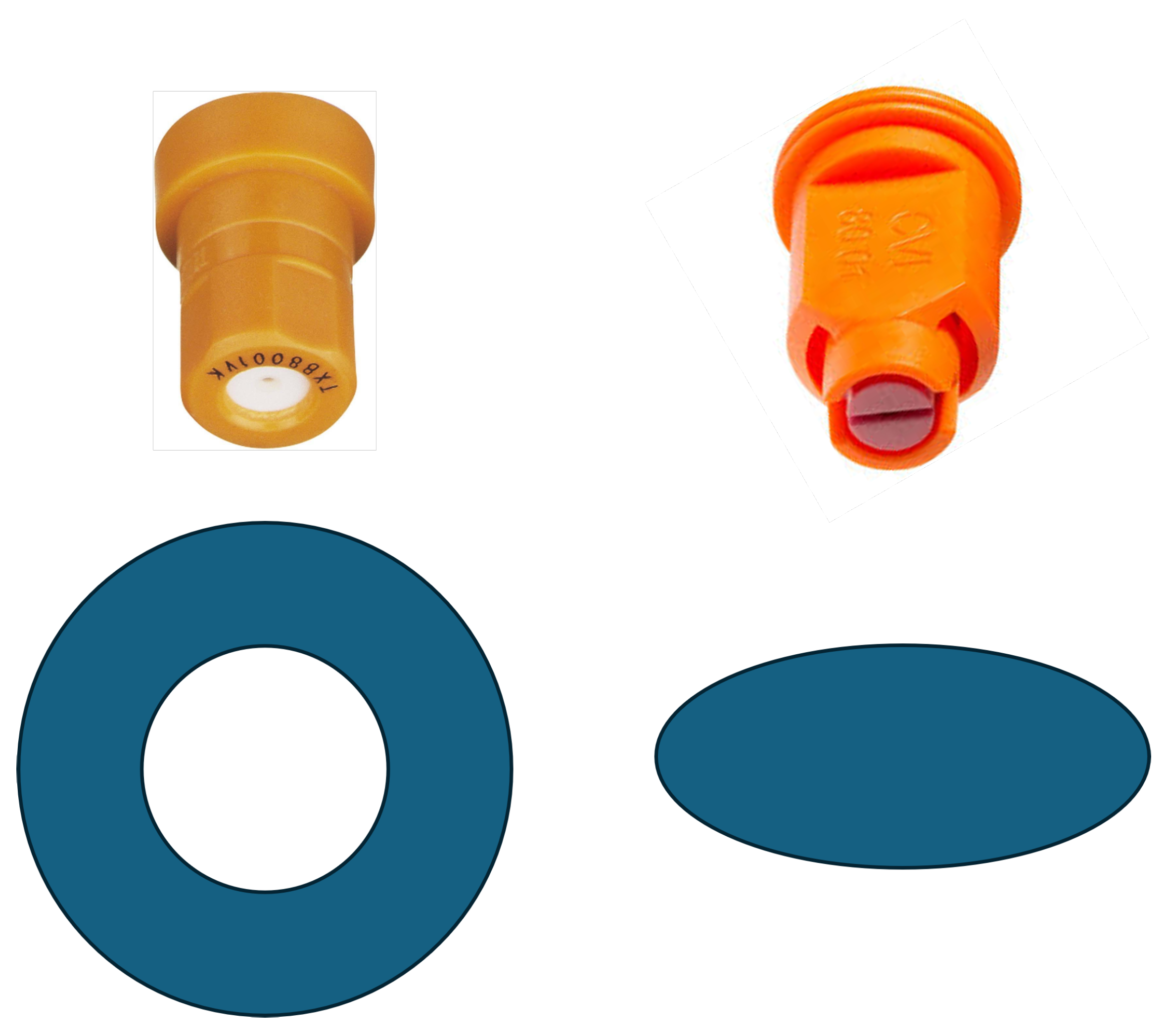
2.1. Investigated Nozzles

The experiments involved two sets of different nozzles, differing by mechanism of action and spray geometry: one was a conventional, hollow-cone model TXB8001VK by Teejet^® Technologies (Wheaton, IL, USA), henceforth “HC”; and the other was an air-inclusion, flat fan model CVI8001 by Albuz^® Spray (Solcera, Evreux Cedex, France), named “AI” in the following. The nozzles and respective spray shapes are shown in Figure 1. For the scopes of all tests of the present study, clear, tap water without visible solids in suspension was sprayed through the nozzles at 700 $\mathrm{k}$$\mathrm{Pa}$. This choice was made to maintain consistency with the previous work, which employed the same nozzles at the same pressure.

The peculiarity of the air-inclusion nozzle is that it produces larger droplets by encapsulating air during the atomisation process, which are supposedly less susceptible to drift, and which disintegrate on impact ensuring a similar coverage to conventional nozzles. This specific model sprays a flat fan of ellipsoidal cross-section; as opposed to the HC which sprays a hollow cone with a circular, hollow cross-section.

2.2. Nozzle Characterisation by PDIA

The characterisation aimed at obtaining the DSD of the selected nozzles. In previous studies [6,28], single nozzles were mounted in an ad hoc test bench and analysed by a VisiSize N60V PDIA system by Oxford Lasers Ltd. (Didcot, Oxfordshire, UK). More details on the construction of the test bench and general operation of the N60 can be found in [28]. The sampling frequency of the instrument is not directly controllable by the user and varies slightly, depending on the computational power available to the system. The sampling is around 30 frames per second for the mode that was used, with some images being possibly rejected if no droplets are successfully recognised by the algorithm. The test length depends on the amount of successfully identified droplets.

In addition to the previous studies, a specific functionality of the VisiSize software was employed to merge the datasets from single analyses. Specifically, different sections of the spray footprint, equally spaced along the line of sight of the PDIA system, were analysed (6 for HC, 5 for AI). The results of the single “slices” were merged into a single dataset. Three nozzle specimens of each type were analysed in this way. This was needed to obtain the overall datasets of different nozzle specimens, different test repetitions on the same specimen or different cross-sections of the spray fan from a single nozzle.

The approach used in the past studies showed that the nozzle was placed at 30 $\mathrm{c}$$\mathrm{m}$ from the PDIA’s FOV. Inconsistent results on certain nozzles led to the conclusion that, at this distance, the flow could be still evolving and breaking up. Furthermore, the standard magnification setting of 0.58× was deemed satisfactory for sampling some classes of nozzles but proved unreliable in acquiring smaller droplets, as detailed below. More specifically, the resolution of the instrument only allowed to identify droplets above 41 μm, while it was found that some nozzle types can spray a consistent fraction of volume around that diameter.

The information gathered from the CSD data of a nozzle can indicate (i) which fraction of the output volume is contained in droplets whose diameter is less than a specific threshold, and (ii) how accurate the nozzle is in generating droplets of a specific diameter, limiting the generation of coarser or finer ones. Since the dimension of a droplet (more specifically, its surface-to-volume ratio [29]) immersed in air substantially determines the time the droplet will spend mid-air [30], it is well known that finer droplets will be more susceptible to drift away from the treated area. Therefore, the volume fraction, denoted as $V_y$, where y is the corresponding diameter in μm, can aid in assessing the “driftability” of a nozzle, once a suitable threshold has been defined. The many parameters involved in the problem of drift [31] make it unreasonable to find a universal threshold, so a wide range of thresholds can be found across the literature, usually ranging from $V_{100}$ used in [32] to $V_{150}$ employed in [24]. The second piece of information, i.e., the ability to generate droplets of a specific diameter, is effectively conveyed by the volume percentiles, referred to as dV_x, where $x\in [0,1]$. ISO 25358 defines the dV_x as the “droplet diameter where the fraction” x “of the spray volume is in smaller droplet sizes”; in other words, x part the output volume resides in droplets of at most dV_x $\mathsf{\mu }\mathrm{m}\mathrm{i}$n diameter. The Relative Span (RS) is a measure of how dispersed the DSD is, and is calculated from the volume percentiles as follows:

$$RS={\displaystyle \frac{d{V}_{90}-d{V}_{10}}{d{V}_{50}}}$$

(1)

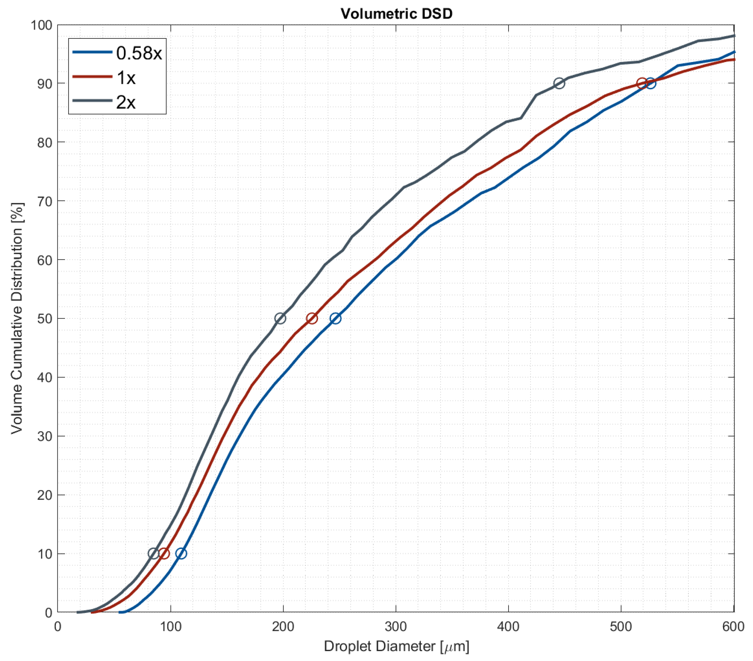
2.3. Toward ISO-Compliance: Optimisation of Instrumental Protocol

ISO 25358:2018 “Droplet-size spectra from atomizers - Measurement and classification” provides guidelines for reliable and repeatable measurements of DSD from agricultural spray nozzles and method for classifying the DSD. The classification is based on commercial nozzles operated with tap water in specific conditions. The DSD of each listed nozzle represents the threshold between two adjacent classes, which range from extra-fine (XF) to ultra-coarse (UC). However, this latter part will not be addressed, as framing the nozzles employed under this classification is out of the scope of this work. This, instead of providing numerical values for the DSD thresholds, ensures that different sampling systems, with different accuracies, in different laboratories all provide the same classification. For this reason, a reliable protocol is crucial. For all the tests listed in this work, the requirement of successful identification of a minimum of 10,000 droplets was enforced. The temperature and relative humidity could not be recorded, but it was ensured to perform the tests in comparable conditions (i.e., consecutively on the same day), with an ambient temperature not deviating from (20 ± 2) °C and humidity not exceeding 50%.

On top of the previous experiences with PDIA [6,17], a comparative analysis has been performed to select the most appropriate hardware-specific instrument settings (namely lens magnification option) and test bench layout.

Three nozzles specimens, model CVI8001, were tested at 700 $\mathrm{k}$$\mathrm{Pa}$, combining two distances from the optical system along the spray fan centreline (300 mm and 400 $\mathrm{m}$$\mathrm{m}$, chiefly constrained by the dimensions of the test bench) and three magnification settings available on the shadowgraph (0.58×, 1×, and 2×); a total of 18 tests was performed, with the data from the different specimens being merged into a unique dataset by the appropriate VisiSize™ functionality. The nozzle type was selected due to its larger droplet diameter range with respect to the HC, as evidenced by previous experiences.

In particular, the questions that motivated this test were as follows:

• Which distance between nozzle orifice and PDIA instrument ensures the sampling of the fully developed flow?
• Which zoom level of the adjustable lens ensures proper sampling of the drop size distributions?

Regarding the first question, ISO 25358 demands that the flow is given sufficient room to properly atomise, suggesting distances between 300 mm and 500 $\mathrm{m}$$\mathrm{m}$. Concerning the second question, each of the lens options can reliably identify droplets in a different diameter range; the three ranges investigated are partially overlapping. The smallest and largest observable equivalent diameters, together with other relevant parameters, of each lens option are reported in

Table 1. Summary of the most relevant parameters for the three standard magnification options under examination. All the data were obtained from the factory calibration files, while the average of particles per frame are referred to the executed tests.

	Lens Magnification Options
	0.58×	1×	2×
Minimum diam. [$\mathsf{\mu }\mathrm{m}]$	41.15	19.26	10.73
Maximum diam. [$\mathsf{\mu }\mathrm{m}]$	3543	2081	1003
Field of view [$\mathsf{\mu }\mathrm{m}$ × $\mathsf{\mu }\mathrm{m}]$	18,662 × 10,631	10,965 × 6246	5280 × 3008
$\mathsf{\mu }\mathrm{m}$-to-pixel factor	9.561	5.617	2.705
Average particles/frame [n]	33.3	11.3	1.3

. The necessity of striking a compromise arises from some points: (a) limiting the loss of too big or too small droplets, ensuring a comprehensive overview of the droplet spectrum; (b) sampling a representative spatial density; (c) ensuring a reasonable duration of the test. The 2× magnification was ruled out, since the trials at this magnification captured an average of 1.3 particles/frame, thus requiring long times to capture a significant number of droplets. All the tests at this magnification barely reached 4000 droplets before being manually stopped after 5 min, while for each other configuration, at least 15,000 droplets were sampled.

2.4. Notes on the Logistic Curve

The logistic curve was formulated in [33] and has ever since seen widespread applications in many fields. Reference [34] successfully employed it to model the CSD of conventional, hollow cone spray nozzles.

Since this paper deals with curve fitting with respect to droplet diameters, we can express a general form of the logistic function of a variable D as follows:

$$y\left(D\right)={\displaystyle \frac{L}{1+e^{-k(D-D_0)}}}$$

(2)

where L represents the upper asymptote (carrying capacity), k is the slope of the curve, and $D_0$ is a value of D so that the curve reaches half capacity, that is $y\left(D_0\right)=L/2$. In other words, $D_0$ has the same physical meaning of dV₅₀, i.e., the volume-based median diameter (VMD). More coefficients can be included, but this formulation is particularly apt to the treated case: since the CSD of a nozzle is, by definition, ranging from 0 to 1, this first coefficient will be locked at $L=1$. The scope of the work is to fit the other two coefficients, k and $D_0$.

2.5. Data Fitting

Data for the two nozzle types were fitted with both models proposed, comparing the goodness of fit, in a similar fashion to what was done by [34]. Having tested three nozzle specimens (cfr. Section 2.2), and therefore having three datasets for each nozzle type, two were used to fit the coefficients, and the remaining one was used to validate the resulting model. The original, separated datasets used in this phase of the work are visualised, for reference, in Figure 2. The datasets present similar, yet not totally superimposed, behaviours, and are therefore apt at performing and evaluating the fits and their respective robustness. Especially the AI data manifest a certain variability in the steepness of the curve, which suggests that a relatively simple expression like the logistic function will not be able to capture the whole diversity in nozzle behaviour. By definition of cumulative distribution, the curves should add up to 1; this however did not happen in all datasets. This is a numerical issue possibly due to the calculations implemented in VisiSize, which operate on a limited number of significant digits.

To execute the fitting, a simple MATLAB R2023a pipeline was developed, leveraging the Curve Fitting Toolbox™. The script allows to select the data, initialise the appropriate model to fit and the relative options, execute the fitting and compare the results. Data are imported from the VisiSize automated test reports as per [28] into a structure array.

The first two structures in the array are fitted separately, handing two separate fitted models with the respective goodness of the fitted (GoF) results. The GoF metrics which will be used are $R^2$ and the Root Mean Square Error (RMSE). The coefficients obtained in the two training fittings are then averaged and used to build a third, new model, using the last structure for validation. The GoF of this third fitting is then calculated.

3. Results and Discussion

3.1. Validation of New Methodology

Figure 3 illustrates the Cumulative Size Distributions (CSDs) at 400 mm, for a qualitative comparison of the effect of magnification presented in

Table 2. Summary of the results from the methodological tests, averaged across the tested specimens. The volume percentiles dV_xx are expressed in $\mathsf{\mu }\mathrm{m},$ while the volume fractions V_yy are in percentage.

Mag.	Distance [mm]	dV10	dV50	dV90	V100	V200
0.58×	300	109.8	311.0	584.0	7.1	31.1
0.58×	400	117.2	256.2	527.1	5.9	38.6
1×	300	95.2	278.8	567.8	11.6	36.7
1×	400	96.4	243.6	546.4	11.1	42.5
2×	300	93.8	227.7	476.5	12.1	44.0
2×	400	95.1	212.9	462.6	11.8	47.1

. Apart from the 2× configuration, the remaining are quite similar, especially as the volume increases.

Table 2 reports the volume percentiles and volume fractions of each test configuration, averaged across the three nozzle specimens. From these results and Figure 3, some considerations can be drawn. At 300 mm, the flow appears to be still developing; despite negligible differences in dV10 or 90, the dv50 appears to significantly vary with distance. Also the effect of magnification is evident. With larger magnifications, more droplets are sampled in the lower range, and less in the coarser range; this has an expected impact on the percentiles. The 0.58× appears very susceptible to this issue, with the V₁₀₀ at both distances being heavily different from those of the other configurations. The 2× was ruled out for the reasons above, i.e., the much higher sampling time, reinforced by the insignificant differences in volume fractions with respect to 1×. The effective sampling domain (i.e., minimum to maximum diameters) of 0.58× is way larger than needed, while the sampled nozzle’s CSD only spans the smaller end of this domain; therefore, the magnification level lacks accuracy in the region of most interest. A similar, yet less pronounced consideration applies to 1×, while 2× clearly lacks the ability to recognise larger droplets, which may happen to be generated by other nozzle types. Of course, using different magnifications for different nozzles would ensure an accurate analysis, but would hinder the consistency of the analyses across different nozzles. This is a further ground to avoid employing the 2× zoom.

In light of these considerations, we proceeded to analyse the nozzles for the experiment at 1× magnification and the highest distance between the instrument’s FOV and the nozzle’s orifice allowed by the bench structure, which was increased to 460 mm.

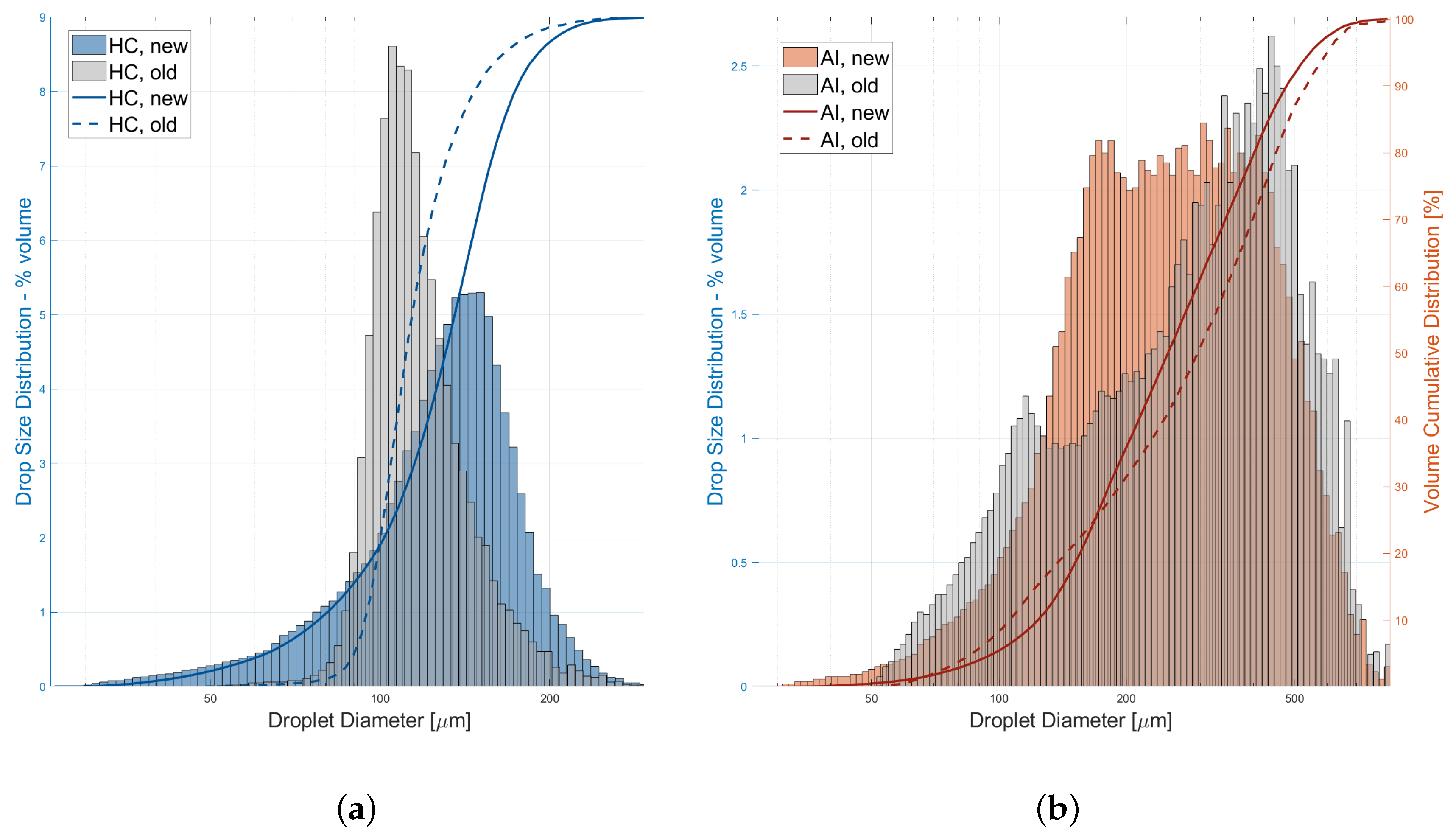
3.2. Data from New Methodology: Comparison with Old

Table 3. Comparison of the results from the two nozzles and the two methodologies, new and old, with respect to the most significant parameters: successfully counted droplets, minimum and maximum equivalent diameters (in $\mathsf{\mu }\mathrm{m})$, volume percentiles dV_xx expressed in $\mathsf{\mu }\mathrm{m},$ the relative span calculated per Equation (1), and volume fractions V_yy (indicated as percentages).

	HC, Old	HC, New	AI, Old	AI, New
In-focus count	45,293	180,313	45,056	130,982
Min. diameter	48.2	26.9	48.5	25.7
Max. diameter	297.4	353.3	932.5	818.8
dV10	94.1	78.0	106.0	123.6
dV50 (VMD)	111.4	130.9	295.0	251.2
dV90	149.8	176.1	533.5	479.1
RS	0.50	0.75	1.45	1.42
V50	<0.01	2.3	N/A	0.5
V100	21.9	21.1	8.3	5.5
V150	90.1	71.4	21.2	18.1
V200	98.5	96.3	31.5	35.8

summarises the relevant nozzle parameters as evaluated with the old and new methodologies.

The considerations outlined in [17] still fundamentally hold. As expected, the DSD of AI nozzles span quite a large diameter domain, while conventional HC nozzles are more accurate in producing a droplet spectrum sharply centred on a specific mean diameter. The difference in performance is qualitatively evident when comparing the distributions in Figure 4 and Figure 5.

With the old methodology, the V₅₀ of both nozzles could not be evaluated, as the minimum diameters were around 48.2 $\mathsf{\mu }\mathrm{m}$ and 48.5 $\mathsf{\mu }\mathrm{m}$ for HC and AI, respectively. As expected, with the increased magnification, these values descend to 26.9 $\mathsf{\mu }\mathrm{m}$ and 25.7 $\mathsf{\mu }\mathrm{m}$ for HC and AI, respectively. It is curious how in both scenarios, these values agree substantially for the two nozzle types, despite the instrument’s minimum recognisable equivalent diameter being declared as lower in both cases (41.2 $\mathsf{\mu }\mathrm{m}$ and 19.2 $\mathsf{\mu }\mathrm{m}$ for 0.58× and 1×, respectively). This is probably due to the increased difficulty in sampling smaller droplets. The larger amount of finer droplets from the conventional nozzles is however confirmed by the steepness of the corresponding CSD in Figure 5b (it should be noted that a steeper curve means that the cumulative volume is significantly increasing as each consecutive dimensional class is added to the computation).

The maximum diameters are widely different and both are abundantly below the maximum diameter recognisable by the instrument (3530 μm and 2081 $\mathsf{\mu }\mathrm{m}$, respectively), which is in agreement with the different atomisation mechanism.

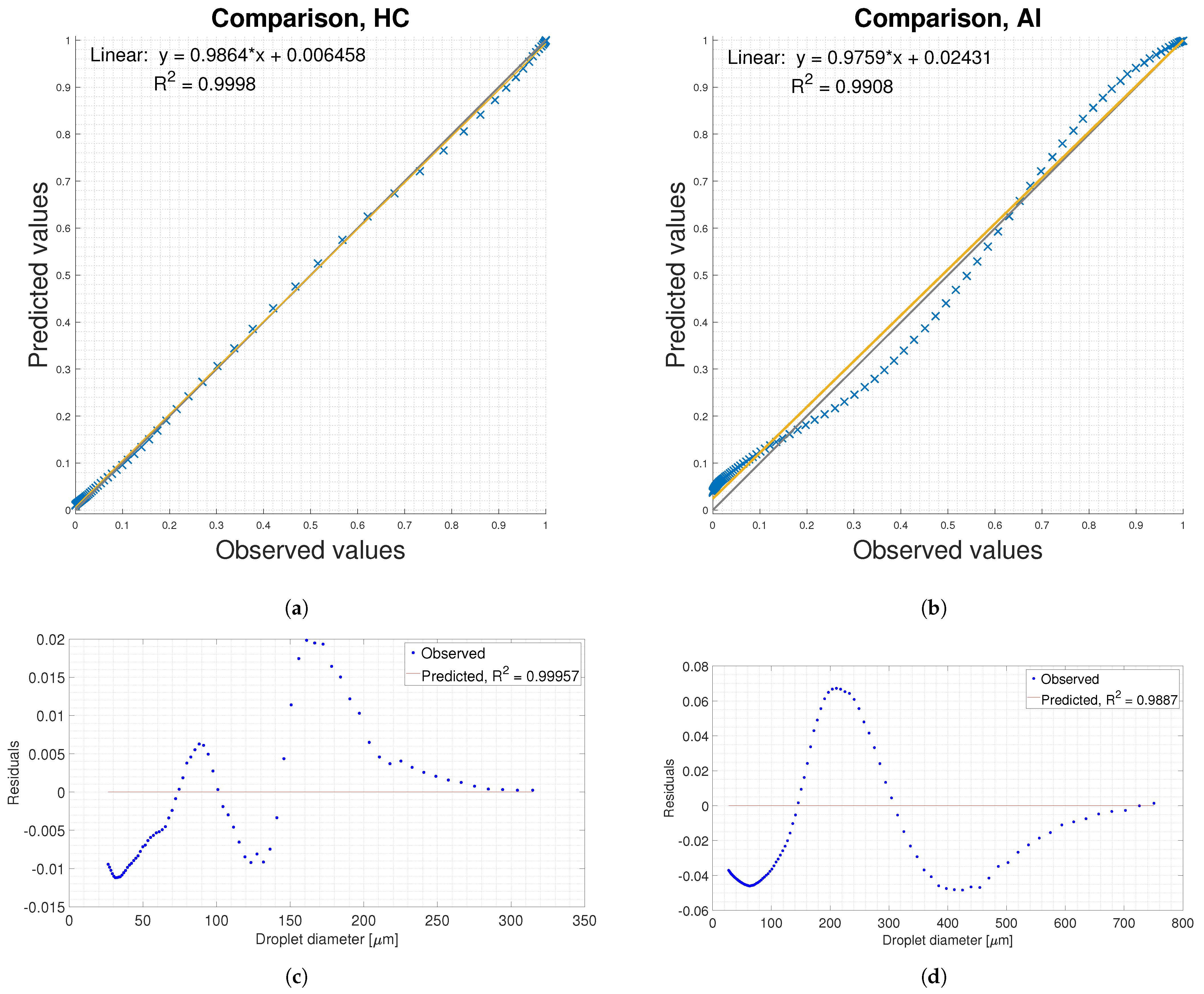
3.3. Data Fitting with Logistic Curve

Table 4. The fitting results for the two nozzle types: average GoF metrics of the training fittings, the average fitting parameters, and the GoF of the validation on the third dataset.

	HC	AI
R2, training	0.9995	0.9863
RMSE, training	0.0091	0.0437
k	0.0451	0.0136
$D_0$	129.65	266.65
R2, validation	0.9996	0.9887
RMSE, validation	0.0086	0.0396

lists, for both nozzle types, the GoF metrics of the training fittings and relative coefficients, averaged across the two couples of training datasets, and the GoF metrics of the validation on the third dataset. The resulting plots are also illustrated in Figure 6.

The trainings showed very good results for both cases and all datasets. This is shown in Figure 6a,b, which also recalls the R² of the single training fits. Here, the blue dots represent the experimental datasets, and the red lines are the obtained fits.

As for the coefficients obtained by averaging the training fittings, the general outcome is satisfactory.

The steepness coefficient k is, predictably, much higher (about three times as much) for HC nozzles, which shows a more compact CSD.

As mentioned in Section 2.4, $D_0$ has the same physical meaning of dV₅₀; therefore, it makes sense to compare the fitted $D_0$ with the dV₅₀ of the datasets. HC nozzles show a good agreement, with 129.7 $\mathsf{\mu }\mathrm{m}$ being calculated against the average 130.5 $\mathsf{\mu }\mathrm{m}$ observed in the datasets. The same cannot be said for AI nozzles, with 253.9 μm and 266.7 $\mathsf{\mu }\mathrm{m}$, respectively, with a deviation of about 5%.

Given the good quality of the fits described above and the similarity in the datasets shown in Figure 2, it is to be expected that the validation of the model would respond very well. Figure 6c,d visualises the ability of the constructed models to predict the CSDs of HC and AI nozzles, respectively. The highly satisfactory GoF values are summarised at the bottom of Table 4.

Figure 7a,b compares the values predicted by the averaged fitting models with the respective observed points. In other words, for every observed value $O\left(D_i\right)$ (that is, every data point obtained from the PDIA presented on the abscissa, the predicted value $P\left(D_i\right)$ at the corresponding diameter $D_i$ is plotted. An ideal, perfect fit would configure a straight diagonal line in this type of plot. The straight line interpolating the data points would need to have a slope as close to 1 as possible, and an intercept as close as possible to 0. This type of visualisation is very illustrative of the irregularities in the observed data, and of how able a fit can be in representing those irregularities. Figure 7a,b also presents the interpolant lines (yellow) and their equations: for HC, this line is virtually indistinguishable from the x-y diagonal, whereas for AI, a slightly off slope and a non-zero intercept remark the considerations outlined above.

Figure 7c,d shows the residuals of the two fittings. The model, applied to both nozzle types, shows a larger divergence toward the lower end of the diameter domain, specifically, below 100 $\mathsf{\mu }$$\mathrm{m}$. The residuals seem to hit their largest values toward the centre of the domain, to then converge at 0 in both cases as the diameters increase. The magnitude of the residuals is much larger for the model applied to AI nozzles, reaching about 6% near the 200 $\mathsf{\mu }$$\mathrm{m}$ mark and about −5% near the 400 $\mathsf{\mu }$$\mathrm{m}$ mark, hinting at a certain margin for improvement, which is in agreement with the previous considerations. In comparison, HC nozzles did not exceed 2%, at about 150 $\mathsf{\mu }$$\mathrm{m}$.

As anticipated above, the AI data exhibited nuances much harder to represent by a simple model like the logistic function, with respect to the HC ones.

In general, HC nozzles allowed for a very tight, almost perfect fit; AI nozzles presented some irregularity, and the relative attempts at fitting are less ideal. However, they can be considered satisfactory, given the very favourable GoF.

The major concern arises at the lower diameters, where a substantial disagreement appears, again especially pronounced in the case of AI.

4. Conclusions & Future Perspectives

The present work recounted the recent experiences at the Innovations Laboratory of the Free University of Bozen-Bolzano in characterising and modeling the behaviour of agricultural nozzles. A reliable, ISO-compliant methodology has been tailored to the available PDIA system, and the resulting data have been employed to develop a data-fitting methodology leveraging a logistic function. Data fitting of nozzle data allows for the development of models and their behaviour, enabling larger simulations of sprayer performance which can aid in both research and support in decision making. As a fitting model, this work considers a basic formulation of the logistic function, which other authors have shown to be suitable for the purpose. De facto, using only two parameters, the model proves quite simple, intuitive and light.

The new PDIA protocol samples the whole footprint of several nozzle specimens, and takes into consideration a much higher number of particles. It exhibits higher reliability with respect to the previous work when applied to two different nozzle types and spray geometry.

A fitting routine has been validated, using some of the datasets collected during the ISO-compliant sampling to train a model and the remaining to validate it. The fitting with the logistic curve proved very accurate for the hollow cone (HC) nozzles ($R^2>0.99$), while some inaccuracies arise with the air-inclusion flat fan (AI) ones, mostly due to the more chaotic droplet generation mechanism which involves the entrainment of air. These inaccuracies are minor; the resulting model is satisfactory and repeatable against the tested datasets ($R^2=0.98$), but it fails to capture the peculiar behaviour of this type of nozzle, especially toward the lower diameters. More in-depth studies would be required in the vision of a more complicated decision support system, to which this issue may constitute a limitation, depending on the desired level of detail. Given the importance of smaller droplets for the generation of drift, actions could be taken to improve the GoF at lower diameters. One example could be inserting a weight system in the fit, to force the algorithm to give priority to the lower diameters. Another way could be represented by a complication of the model, possibly adding parameters, but the increased effort has to be compromised against the benefits. For the moment, therefore, both fittings can be deemed highly satisfactory, especially since the main aim of this part of the work was to develop a reliable methodology to potentially treat larger amounts of datasets. The next steps include the improvement of the model as outlined above, to investigate the influence of operating pressure and to deploy the model to larger scale evaluations, integrating these results with other aspects of the sprayer’s performance such as the air distribution. This goes in the direction of building a generalised performance model of the sprayer to simulate its working in different conditions and configurations. Such a modeling effort can have potential benefits on all links of the lifecycle of the sprayer, from support to research and development for manufacturers to training and increased awareness of end users on the importance of the parameters under their control. Further studies are underway to apply a similar fitting procedure to aerosol data, trying to analyse patterns in the behaviour of the generated spray cloud as a function of nozzle type and distance from the sprayer, as well as similarities between the nozzle performance and composition of the aerosol cloud.

References

1. Hilz, E.; Vermeer, A.W. Spray Drift Review: The Extent to Which a Formulation Can Contribute to Spray Drift Reduction. Crop Prot. 2013, 44, 75–83. [Google Scholar] [CrossRef]
2. Torrent, X.; Gregorio, E.; Douzals, J.P.; Tinet, C.; Rosell-Polo, J.R.; Planas, S. Assessment of Spray Drift Potential Reduction for Hollow-Cone Nozzles: Part 1. Classification Using Indirect Methods. Sci. Total Environ. 2019, 692, 1322–1333. [Google Scholar] [CrossRef] [PubMed]
3. Tudi, M.; Daniel Ruan, H.; Wang, L.; Lyu, J.; Sadler, R.; Connell, D.; Chu, C.; Phung, D.T. Agriculture Development, Pesticide Application and Its Impact on the Environment. Int. J. Environ. Res. Public Health 2021, 18, 1112. [Google Scholar] [CrossRef] [PubMed]
4. Perine, J.; Anderson, J.; Kruger, G.; Abi-Akar, F.; Overmyer, J. Effect of Nozzle Selection on Deposition of Thiamethoxam in Actara® Spray Drift and Implications for Off-Field Risk Assessment. Sci. Total Environ. 2021, 772, 144808. [Google Scholar] [CrossRef] [PubMed]
5. Ferguson, J.C.; O’Donnell, C.C.; Chauhan, B.S.; Adkins, S.W.; Kruger, G.R.; Wang, R.; Urach Ferreira, P.H.; Hewitt, A.J. Determining the Uniformity and Consistency of Droplet Size across Spray Drift Reducing Nozzles in a Wind Tunnel. Crop Prot. 2015, 76, 1–6. [Google Scholar] [CrossRef]
6. Becce, L.; Mazzi, G.; Ali, A.; Bortolini, M.; Gregoris, E.; Feltracco, M.; Barbaro, E.; Contini, D.; Mazzetto, F.; Gambaro, A. Wind Tunnel Evaluation of Plant Protection Products Drift Using an Integrated Chemical–Physical Approach. Atmosphere 2024, 15, 656. [Google Scholar] [CrossRef]
7. Cunha, J.P.A.R.D.; Lopes, L.D.L.; Alves, C.O.R.; Alvarenga, C.B.D. Spray Deposition and Losses to Soil from a Remotely Piloted Aircraft and Airblast Sprayer on Coffee. AgriEngineering 2024, 6, 2385–2394. [Google Scholar] [CrossRef]
8. Palma, R.P.; Cunha, J.P.A.R.D. Multivariate Analysis Applied to the Ground Application of Pesticides in the Corn Crop. AgriEngineering 2023, 5, 829–839. [Google Scholar] [CrossRef]
9. Nuyttens, D.; Zwertvaegher, I.K.; Dekeyser, D. Spray Drift Assessment of Different Application Techniques Using a Drift Test Bench and Comparison with Other Assessment Methods. Biosyst. Eng. 2017, 154, 14–24. [Google Scholar] [CrossRef]
10. Jomantas, T.; Lekavičienė, K.; Steponavičius, D.; Andriušis, A.; Zaleckas, E.; Zinkevičius, R.; Popescu, C.V.; Salceanu, C.; Ignatavičius, J.; Kemzūraitė, A. The Influence of Newly Developed Spray Drift Reduction Agents on Drift Mitigation by Means of Wind Tunnel and Field Evaluation Methods. Agriculture 2023, 13, 349. [Google Scholar] [CrossRef]
11. Wang, G.; Han, Y.; Li, X.; Andaloro, J.; Chen, P.; Hoffmann, W.C.; Han, X.; Chen, S.; Lan, Y. Field Evaluation of Spray Drift and Environmental Impact Using an Agricultural Unmanned Aerial Vehicle (UAV) Sprayer. Sci. Total Environ. 2020, 737, 139793. [Google Scholar] [CrossRef] [PubMed]
12. Bourodimos, G.; Koutsiaras, M.; Psiroukis, V.; Balafoutis, A.; Fountas, S. Development and Field Evaluation of a Spray Drift Risk Assessment Tool for Vineyard Spraying Application. Agriculture 2019, 9, 181. [Google Scholar] [CrossRef]
13. Sapkota, M.; Virk, S.; Rains, G. Spray Deposition and Quality Assessment at Varying Ground Speeds for an Agricultural Sprayer with and without a Rate Controller. AgriEngineering 2023, 5, 506–519. [Google Scholar] [CrossRef]
14. Butler Ellis, M.; Alanis, R.; Lane, A.; Tuck, C.; Nuyttens, D.; Van De Zande, J. Wind Tunnel Measurements and Model Predictions for Estimating Spray Drift Reduction under Field Conditions. Biosyst. Eng. 2017, 154, 25–34. [Google Scholar] [CrossRef]
15. Liu, Q.; Chen, S.; Wang, G.; Lan, Y. Drift Evaluation of a Quadrotor Unmanned Aerial Vehicle (UAV) Sprayer: Effect of Liquid Pressure and Wind Speed on Drift Potential Based on Wind Tunnel Test. Appl. Sci. 2021, 11, 7258. [Google Scholar] [CrossRef]
16. Nuyttens, D.; Taylor, W.; De Schampheleire, M.; Verboven, P.; Dekeyser, D. Influence of Nozzle Type and Size on Drift Potential by Means of Different Wind Tunnel Evaluation Methods. Biosyst. Eng. 2009, 103, 271–280. [Google Scholar] [CrossRef]
17. Becce, L.; Mazzi, G.; Ali, A.; Bortolini, M.; Gambaro, A.; Mazzetto, F. Nozzle Characterisation to Support Aerosol Spray Drift Measurement in a Semi-Controlled Environment. In Proceedings of the 2023 IEEE International Workshop on Metrology for Agriculture and Forestry (MetroAgriFor), Pisa, Italy, 6–8 November 2023; pp. 646–651. [Google Scholar] [CrossRef]
18. Sijs, R.; Kooij, S.; Holterman, H.J.; Van De Zande, J.; Bonn, D. Drop Size Measurement Techniques for Sprays: Comparison of Image Analysis, Phase Doppler Particle Analysis, and Laser Diffraction. AIP Adv. 2021, 11, 015315. [Google Scholar] [CrossRef]
19. Gil, E.; Balsari, P.; Gallart, M.; Llorens, J.; Marucco, P.; Andersen, P.G.; Fàbregas, X.; Llop, J. Determination of Drift Potential of Different Flat Fan Nozzles on a Boom Sprayer Using a Test Bench. Crop Prot. 2014, 56, 58–68. [Google Scholar] [CrossRef]
20. Grella, M.; Marucco, P.; Balsari, P. Toward a New Method to Classify the Airblast Sprayers According to Their Potential Drift Reduction: Comparison of Direct and New Indirect Measurement Methods. Pest Manag. Sci. 2019, 75, 2219–2235. [Google Scholar] [CrossRef]
21. Grella, M.; Gil, E.; Balsari, P.; Marucco, P.; Gallart, M. Advances in Developing a New Test Method to Assess Spray Drift Potential from Air Blast Sprayers. Span. J. Agric. Res. 2017, 15, e0207. [Google Scholar] [CrossRef]
22. Zhang, Z.; Zhu, H.; Guler, H. Quantitative Analysis and Correction of Temperature Effects on Fluorescent Tracer Concentration Measurement. Sustainability 2020, 12, 4501. [Google Scholar] [CrossRef]
23. ISO 25358:2018; Crop Protection Equipment—Droplet-Size Spectra from Atomizers—Measurement and Classification. ISO: Geneva, Switzerland, 2018.
24. Krishnan, G.; Cryer, S.A.; Turner, J.E.; Sasi Rajan, N. Spray Atomisation in Multiphase Flows with Reference to Tank Mixes of Agricultural Products. Biosyst. Eng. 2022, 223, 232–248. [Google Scholar] [CrossRef]
25. Cooper, J.; Smith, D.; Dobson, H. An Evaluation of Two Field Samplers for Monitoring Spray Drift. Crop Prot. 1996, 15, 249–257. [Google Scholar] [CrossRef]
26. Coscollà, C.; Muñoz, A.; Borrás, E.; Vera, T.; Ródenas, M.; Yusà, V. Particle Size Distributions of Currently Used Pesticides in Ambient Air of an Agricultural Mediterranean Area. Atmos. Environ. 2014, 95, 29–35. [Google Scholar] [CrossRef]
27. Radoman, N.; Christiansen, S.; Johansson, J.H.; Hawkes, J.A.; Bilde, M.; Cousins, I.T.; Salter, M.E. Probing the Impact of a Phytoplankton Bloom on the Chemistry of Nascent Sea Spray Aerosol Using High-Resolution Mass Spectrometry. Environ. Sci. Atmos. 2022, 2, 1152–1169. [Google Scholar] [CrossRef]
28. Becce, L.; Amin, S.; Carabin, G.; Mazzetto, F. Preliminary Spray Nozzle Characterization Activities through Shadowgraphy at the AgroForestry Innovation Lab (AFI-Lab). In Proceedings of the 2022 IEEE Workshop on Metrology for Agriculture and Forestry (MetroAgriFor), Perugia, Italy, 3–5 November 2022; pp. 136–140. [Google Scholar] [CrossRef]
29. Lefebvre, A.H.; McDonell, V.G. Atomization and Sprays, 2nd ed.; CRC Press: Boca Raton, FL, USA; Taylor & Francis Group: Milton Park, UK, 2017. [Google Scholar]
30. Gil, Y.; Sinfort, C. Emission of Pesticides to the Air during Sprayer Application: A Bibliographic Review. Atmos. Environ. 2005, 39, 5183–5193. [Google Scholar] [CrossRef]
31. Arvidsson, T.; Bergström, L.; Kreuger, J. Spray Drift as Influenced by Meteorological and Technical Factors. Pest Manag. Sci. 2011, 67, 586–598. [Google Scholar] [CrossRef]
32. Grella, M.; Marucco, P.; Manzone, M.; Gallo, R.; Mazzetto, F.; Balsari, P. Indoor Test Bench Measurements of Potential Spray Drift Generated by Multi-Row Sprayers. In Proceedings of the 2021 IEEE International Workshop on Metrology for Agriculture and Forestry (MetroAgriFor), Trento-Bolzano, Italy, 3–5 November 2021; pp. 356–361. [Google Scholar] [CrossRef]
33. Garnier, J.; Quetelet, A. Correspondance Mathématique et Physique; Number v. 10; M.Hayez, Imprimeur: Lognes, France, 1838. [Google Scholar]
34. Cerruto, E.; Ramírez-Cuesta, J.M.; Privitera, S.; Pascuzzi, S.; Manetto, G. Use of the Logistic Function to Model Cumulative Volumes of Spray Nozzles. In Proceedings of the 2023 IEEE International Workshop on Metrology for Agriculture and Forestry (MetroAgriFor), Pisa, Italy, 6–8 November 2023; pp. 635–639. [Google Scholar] [CrossRef]
Figure 1. View of the two nozzles and a representation of the respective spray geometries: HC (left) and AI (right).
Agriengineering 07 00139 g001
Figure 2. The three original datasets used to fit HC (a) and AI (b) nozzle data, as extracted by the N60 automated test report. The continuous lines represent the cumulative distributions and are obtained by linear interpolation between consecutive data points; the circles identify the 10th, 50th, and 90th volume percentiles.
Agriengineering 07 00139 g002
Figure 3. Cumulative Size Distributions (CSDs) from different magnifications at 400mm. The circles identify the 10th, 50th, and 90th volume percentiles.
Agriengineering 07 00139 g003
Figure 4. Comparison of volumetric DSD and CSD of nozzles across the two methodologies. The gray histograms and dashed lines refer to the old methodology: (a) HC (TXB8001) and (b) AI (CVI8001) nozzles. The scale on the left of each plot is referred to the histograms, on the right to the cumulated curves.
Agriengineering 07 00139 g004
Figure 5. Superposition of the CSDs from both nozzle types and methodologies: (a) overview; (b) close-up of the lower diameters.
Agriengineering 07 00139 g005
Figure 6. Outcomes of the fitting for all nozzle data: (a,c) refer to HC nozzles and (b,d) to AI nozzles. (a,b) Training with the first two datasets for each type, and (c,d) validation on the third dataset.
Agriengineering 07 00139 g006
Figure 7. Outcomes of the fitting for all nozzle data (continued): (a,c) refer to HC nozzles, (b,d) to AI nozzles. (a,b) Compare the observed (experimental) and predicted (fitted) values, presenting (yellow lines) the linear interpolants of the data points and the respective equations; (c,d) plot the residuals of the resulting models. Notice the different values on the y-axis, once again substantiating the different quality of the fits.
Agriengineering 07 00139 g007