2.1. Optimizing Sampling Intervals for Energy-Efficient Sensor Operation
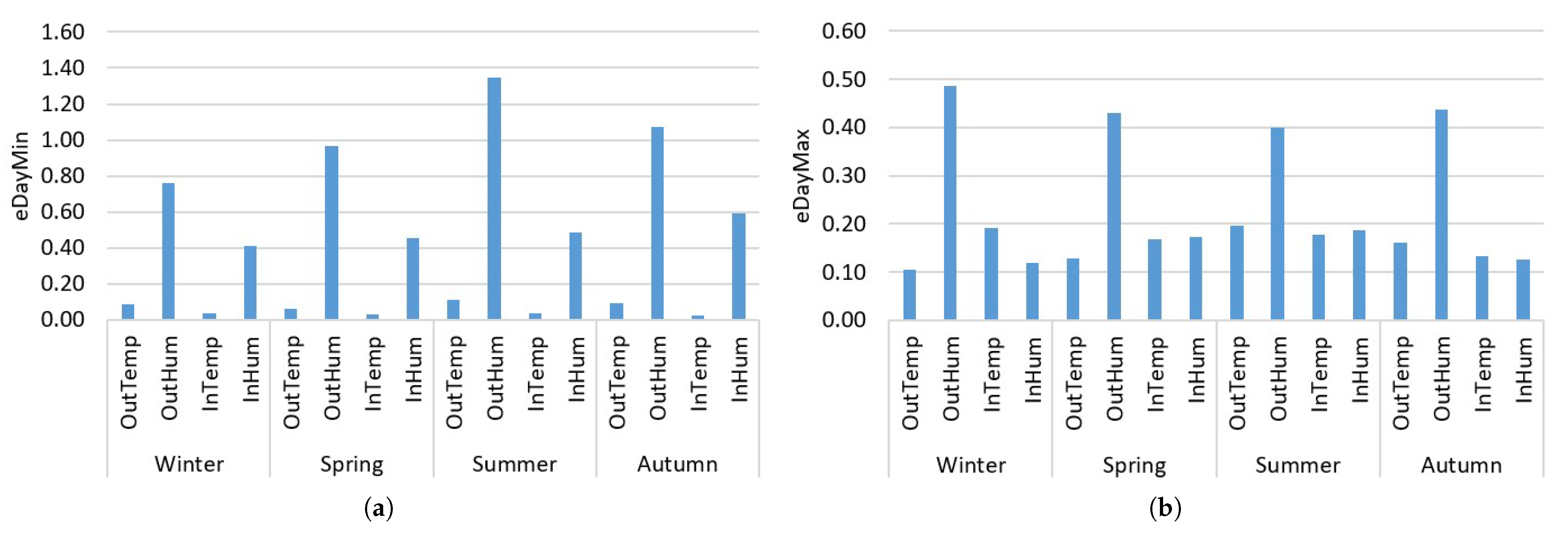
To optimize the energy consumption of sensors installed in greenhouses, we firstly determine the optimal sampling time for the environmental parameters that we aim to monitor. In this study, we have analyzed and monitored temperature and humidity, both external and internal, across four different greenhouses located in the same area.
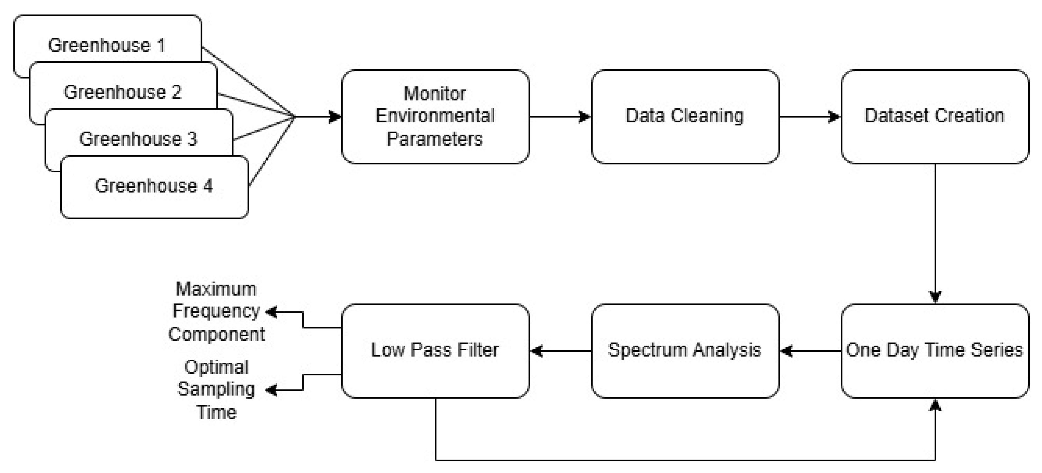
Figure 1 illustrates the workflow followed for the sampling time analysis.
In general, the workflow for determining the optimal sampling time of the monitored parameter can be applied to any time series values and is independent of the specific scenario in which it is implemented, such as the type of greenhouse or sensor used. The parameter for which the optimal sampling interval was determined was first monitored by collecting and storing samples in a database. Once the dataset is created, it undergoes analysis by dividing it into daily segments. For each day, the signal spectrum is computed using transformations such as the Discrete Fourier Transform (DFT), Fast Fourier Transform (FFT), Short-Time Fourier Transform (STFT), Wavelet Transform, or Hilbert Transform. These methods differ in terms of resolution, computational speed, and time–frequency analysis capabilities. In this study, as detailed later, the DFT is employed due to its simplicity and the fact that the signal under analysis is discrete in time. The variation in climate, depending on the location and region, affects the spectrum of the sampled signal. If the parameter exhibits greater fluctuations within the analysis window, the frequency spectrum will be broader, and vice versa. The frequency spectrum is then filtered to remove irrelevant signal frequencies. Finally, to determine the specific sampling interval for the selected time window, the well-known Nyquist theorem is applied.
More specifically, we began by monitoring and collecting temperature and humidity data provided by the greenhouse sensors with a sampling interval of 5 min (as explained in detail in
Section 3.1), which we assume to be significantly smaller than the optimal sampling interval since the average variation between consecutive samples is very low, as demonstrated in
Section 3.1, providing minimal additional information. After collecting the data, we cleaned any errors or missing entries encountered during transmission, creating a dataset that serves as the reference for this study.
During the data analysis process, we first divided the data into daily subsets and then processed them by applying the Discrete Fourier Transform (DFT), as described in Equation (
1). The DFT is the most important discrete transform used for Fourier analysis in many practical applications. In digital signal processing, a function represents any quantity or signal that varies over time (e.g., the pressure of a sound wave, a radio signal, or daily temperature readings) sampled over a finite time interval. The DFT transforms a sequence of
N complex numbers
into another sequence of complex numbers
.
where
is the signal represented in the frequency domain. After computing the signal spectrum, it is passed through a low-pass filter, retaining only the portion of the spectrum where the majority of the signal’s energy resides. At this stage, the maximum spectral frequency (
) and the optimal sampling time (
) for the day can be extracted using Equation (
2), considering the Nyquist theorem. The theorem states that the sampling frequency must be at least twice the maximum frequency component of the signal being sampled to accurately reconstruct the original signal.
Once
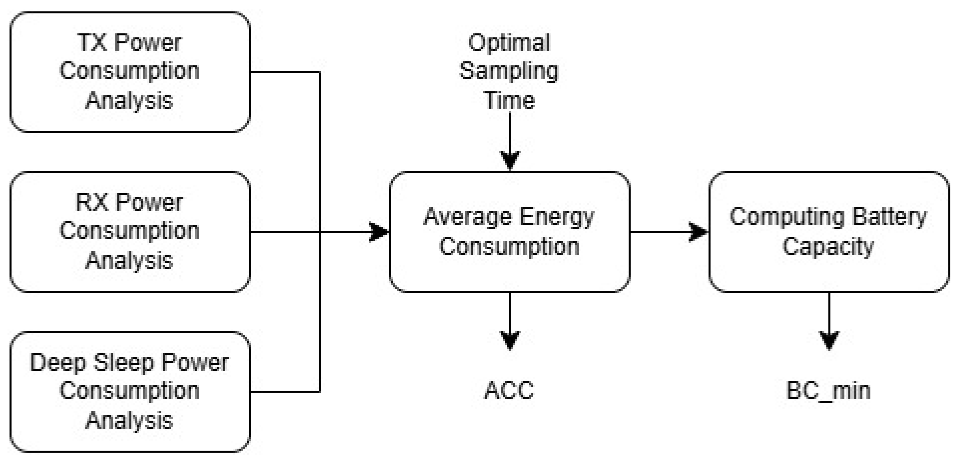
is calculated on a day-by-day basis, the next step involves performing an energy analysis of the individual Micro-Controller Unit (MCU) board to which the sensor is connected, in order to optimize its energy consumption. The steps followed for this analysis are outlined in
Figure 2.
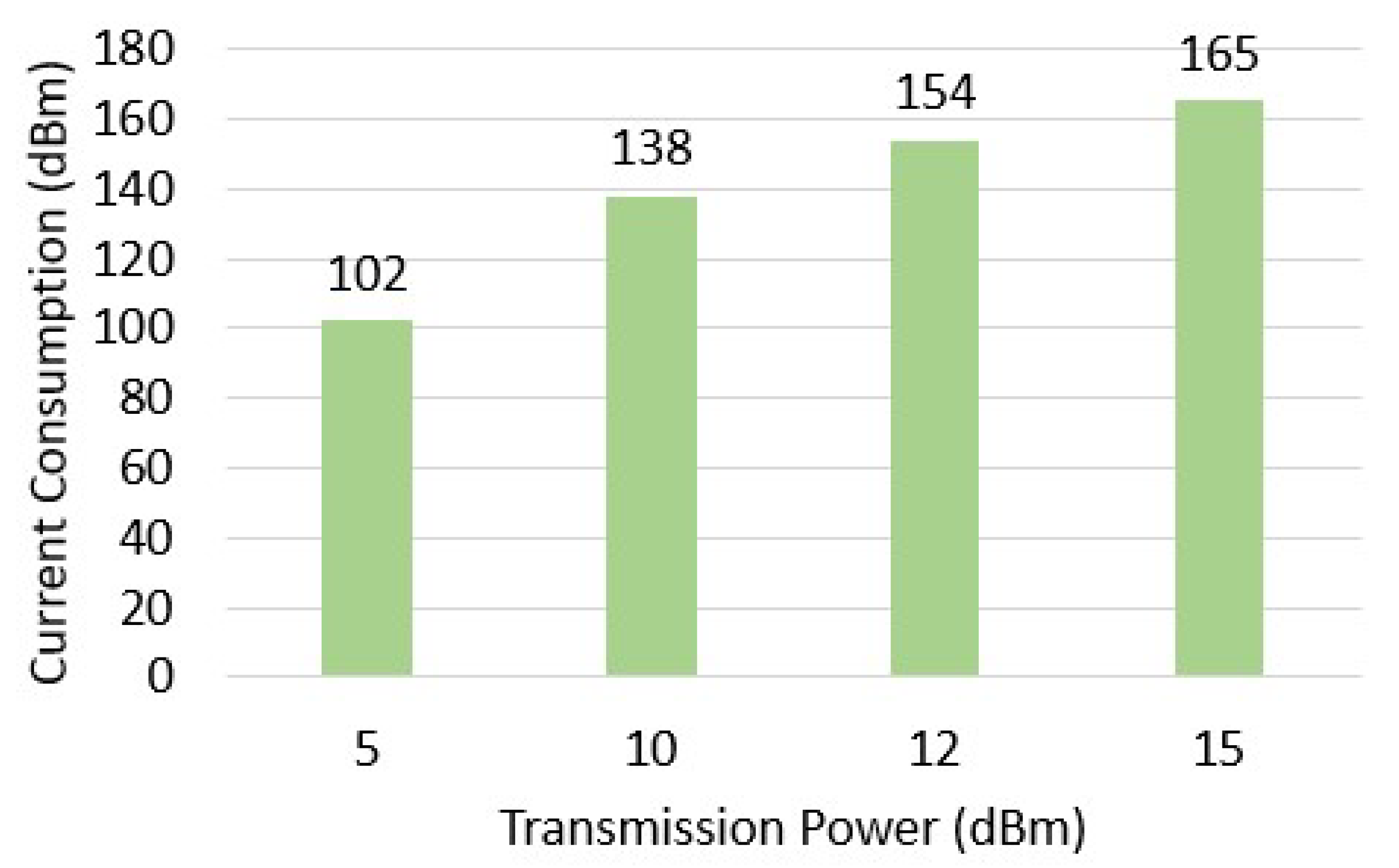
Upon completing the energy consumption analysis, the average current consumption (ACC) can be calculated by measuring the current consumption of the MCU board in its various states and then applying Equation (
3).
Here,
represents the current consumed in transmission mode,
in receiver mode, and
in deep sleep mode. Meanwhile,
is the time taken to transmit the message, and
is the sampling period of the environmental parameter.
At the end, based on the duration of sunlight (
) and night-time (
) hours in the greenhouse, Equation (
4) can be used to calculate the minimum battery capacity (
) required to provide sufficient energy for the MCU board to operate throughout the night, assuming that sufficient energy is harvested during the day to power the board, as is the case in our work.
2.2. Design of the Energy Harvesting System
We assumed the presence of high-power LEDs in a smart greenhouse to provide artificial illumination even when sunlight is low or absent [
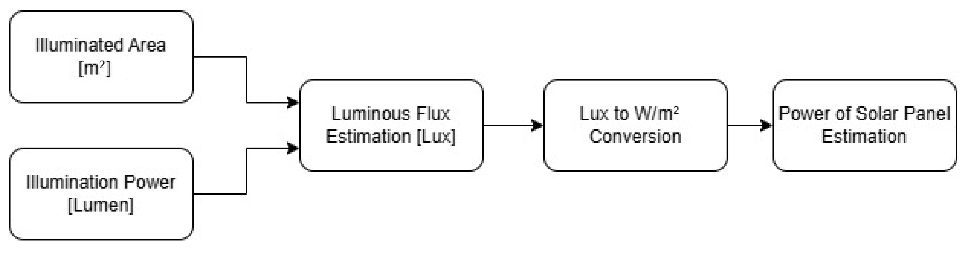
25]. To make the duration of the MCU board independent from battery life, we have proposed the workflow, as shown in
Figure 3. The goal is to convert and reuse the energy emitted by the lamps and external sources, such as sunlight, using small solar panels directly attached to the individual MCU boards. The aim is to fully power the boards during the day and recharge the mini battery to supply energy during the night, when both lamps and sunlight are absent.
Given the size of the area to be illuminated (A[m
2]) and the optimal lighting power (
[lumen]) required for plant growth (provided by both sunlight and artificial lamps), the estimated luminous flux (
[lux]) can be calculated using Equation (
5).
Then, we convert them from lux to W/m
2 (
) using Equation (
6).
To estimate the current provided by the solar panel (
[A]) with a certain area (
[m
2]), efficiency (
), and provided voltage (
[V]), Equation (
7) is used.
2.3. Materials
To collect environmental data both inside and outside the greenhouses, we utilized a central weather station, the Davis Vantage Pro 2 [
26]. This weather station is capable of measuring wind direction and speed, air temperature with an accuracy of ±0.3 °C, air humidity with an accuracy of ±2%, atmospheric pressure, and rainfall. The data collection system consists of the central station, from which we collect external temperature and humidity data, and four distributed units, each located within a greenhouse, with the same measurement accuracy. The four greenhouses are located in the same area in Pisa, Italy. The data collected from the five stations constitute the dataset under study in this work.
Assuming the same network architecture as in our previous work [
25], the test MCU board used was the Heltec WiFi LoRa v3 [
27], which supports communication via both Wi-Fi and long-range technology (LoRa) at 868 MHz. The studies in the literature demonstrate that LoRa modulation is more energy-efficient compared to Wi-Fi; therefore, in this study, the boards communicate using LoRa modulation. The sensor used to collect air temperature and humidity data were the DHT11 [
28]. The Heltec board was powered by a polycrystalline solar panel from Star Solar, model CNC85x115-18 [
29], with dimensions of 85 mm × 115 mm. The panel delivers a maximum power of 1.5 W, a maximum voltage of 18 V, and a maximum current of 83 mA before being connected to the energy harvesting module EH302 [
30]. To power the board during the night, a Li-Po battery [
31] with a nominal voltage of 3.7 V and a capacity of 1350 mAh was used.
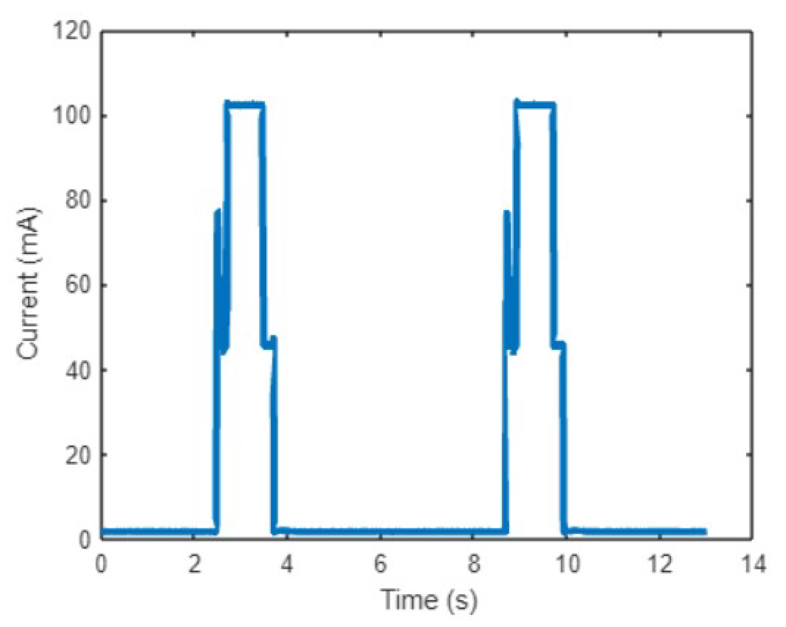
Finally, to analyze the power consumption of the Heltec board, the Qoitech Otii Arc PRO device [
32] was used. This device serves as a two-quadrant source measure unit with constant voltage or constant current sourcing and sinking capabilities. It also features a high-precision multichannel multimeter and a linear power supply (0.5–5 V). The Otii Arc PRO functions as a power analyzer or profiler, enabling real-time recording and display of currents, voltages, and/or UART logs. It provides current measurements with nanoampere resolution and supports a sampling rate of up to 4 ksps.


