


Correlation Between the Growth Index and Vegetation Indices for Irrigated Soybeans Using Free Orbital Images

 , , , ,
  , and
, and 
Abstract
1. Introduction
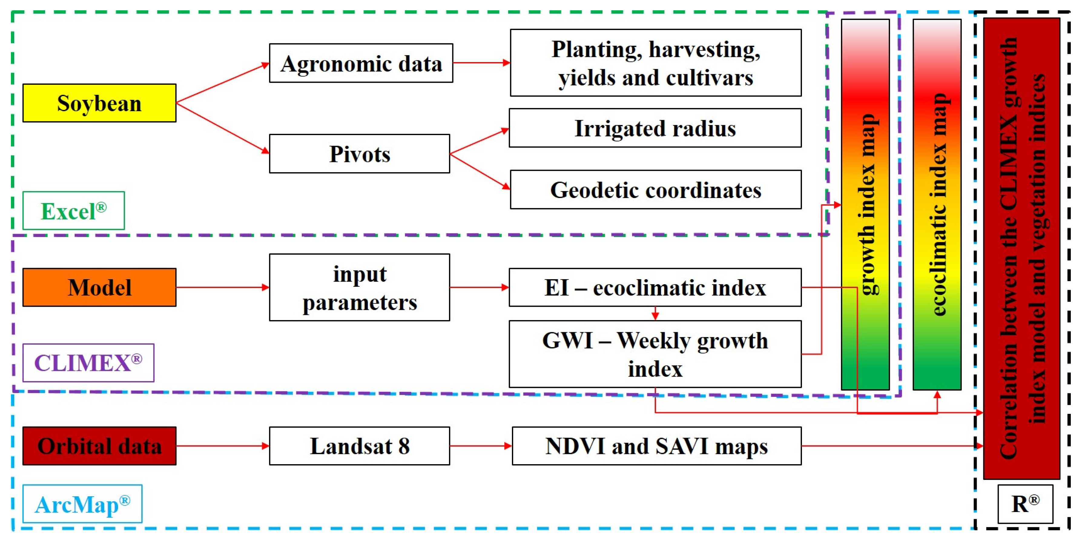
2. Materials and Methods
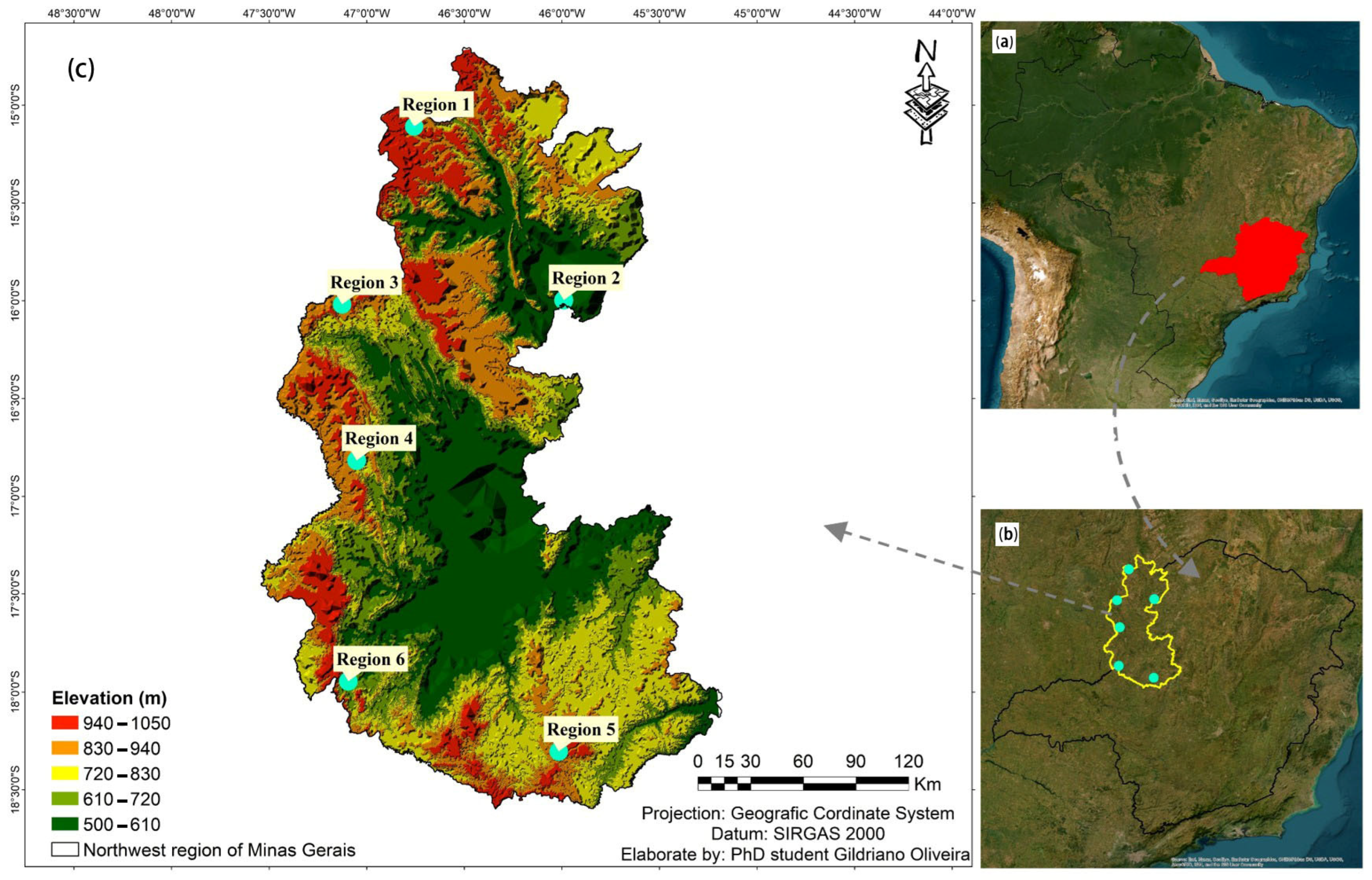
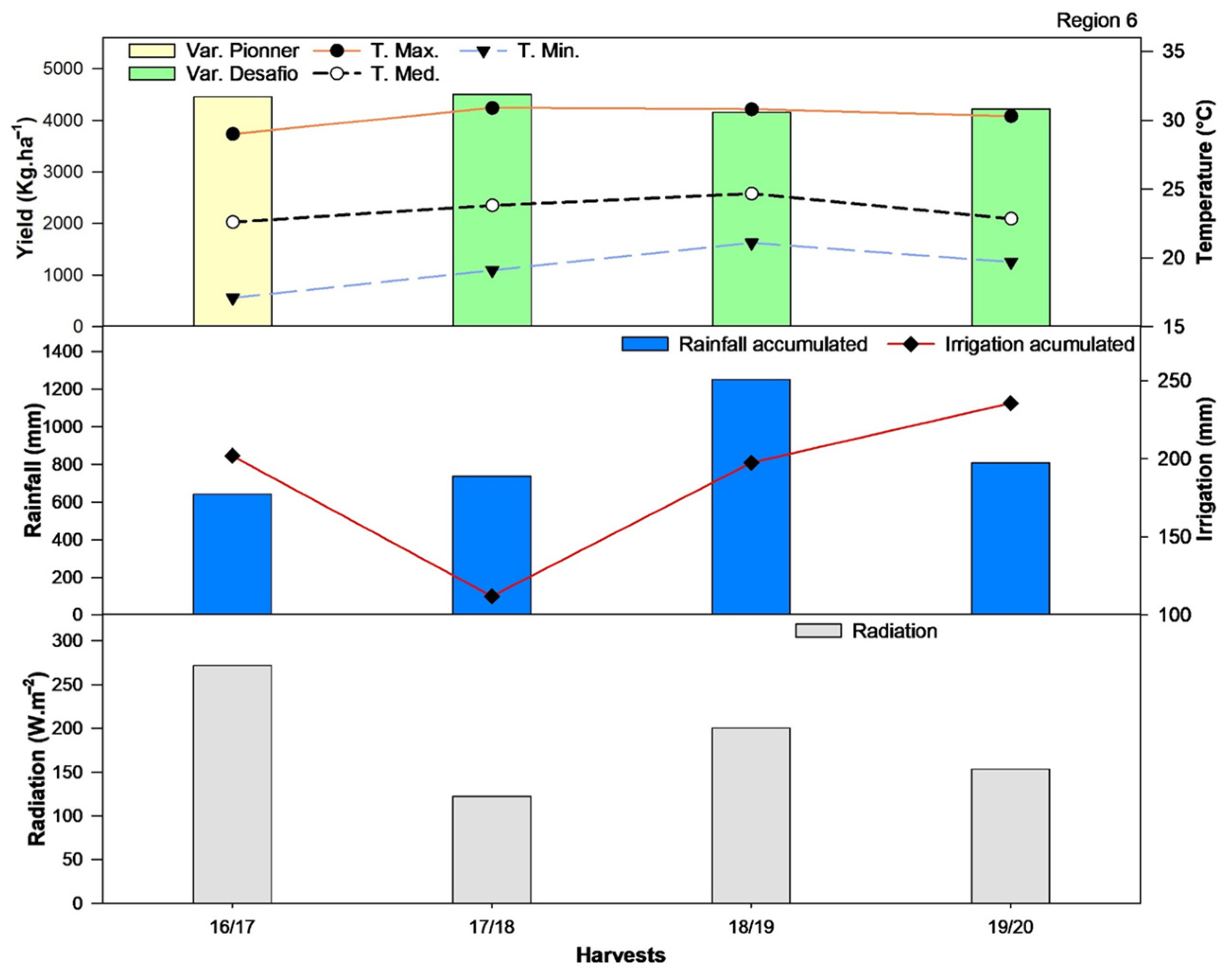
2.1. Study Area
2.2. CLIMEX
2.3. Parameters Used in CLIMEX
2.4. Climatological Data
2.5. Orbital Data and Processing to Determine the Maximum Vegetation Index
2.5.1. Obtaining Vegetation Indices
2.5.2. Image Processing and Statistical Analysis
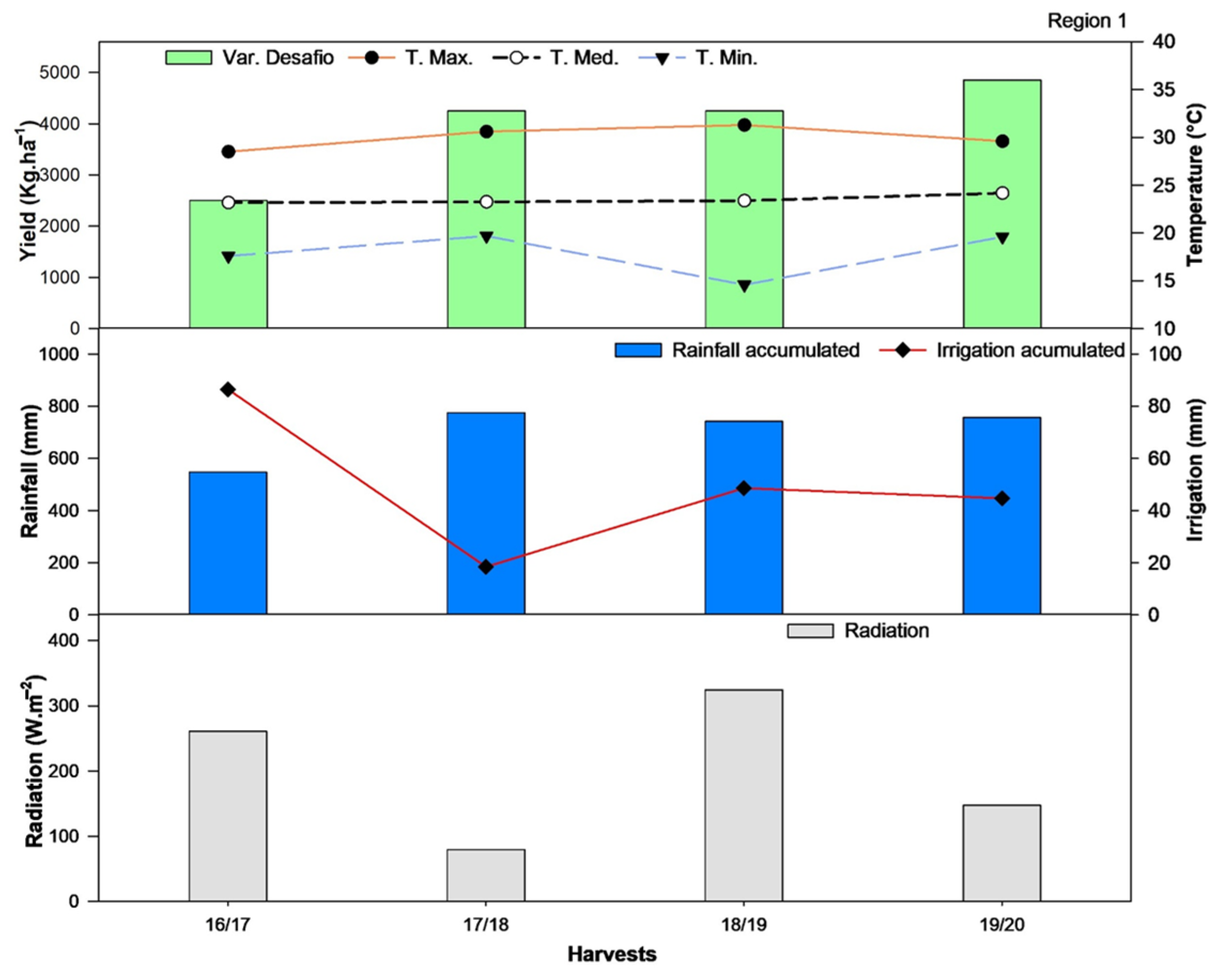
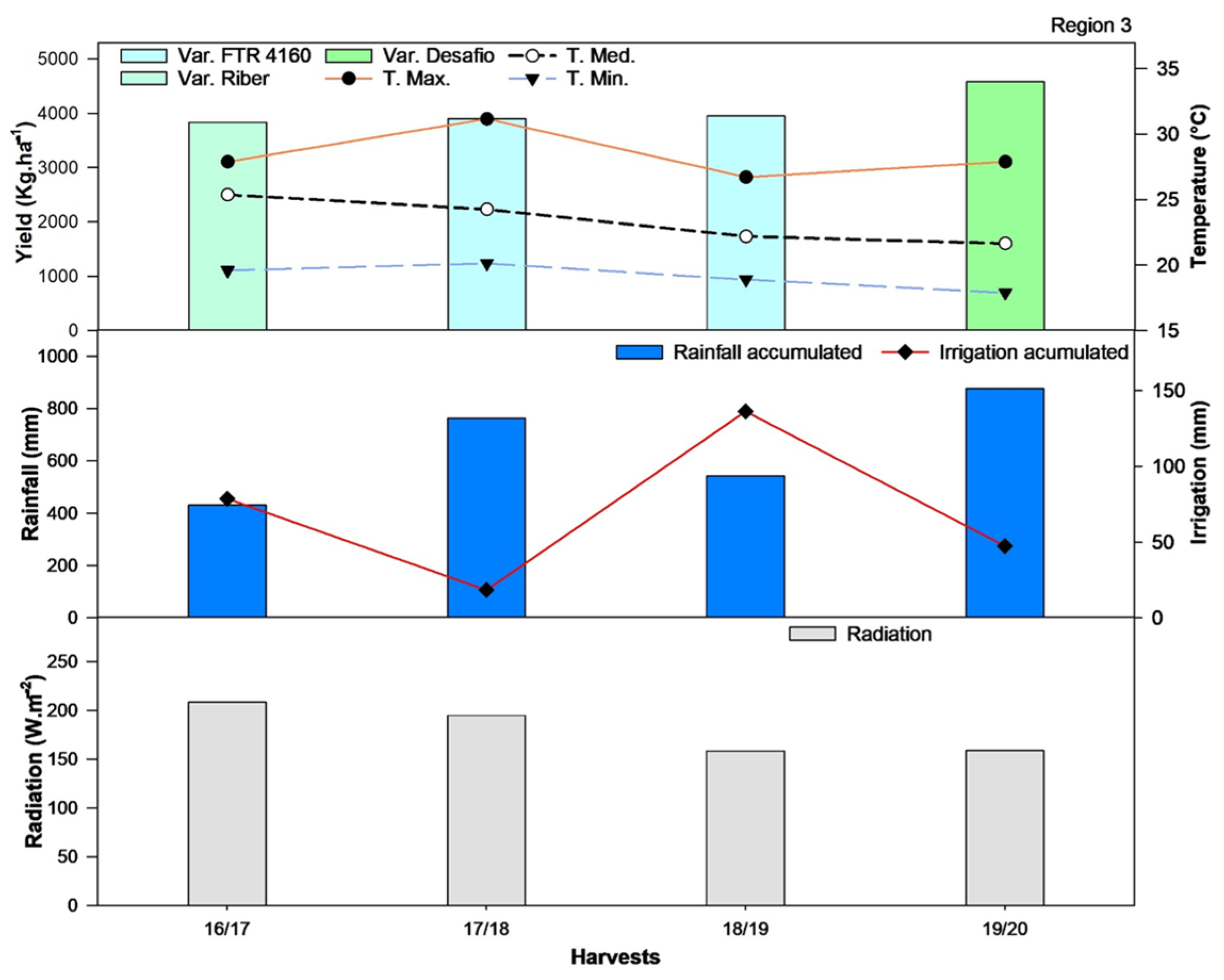
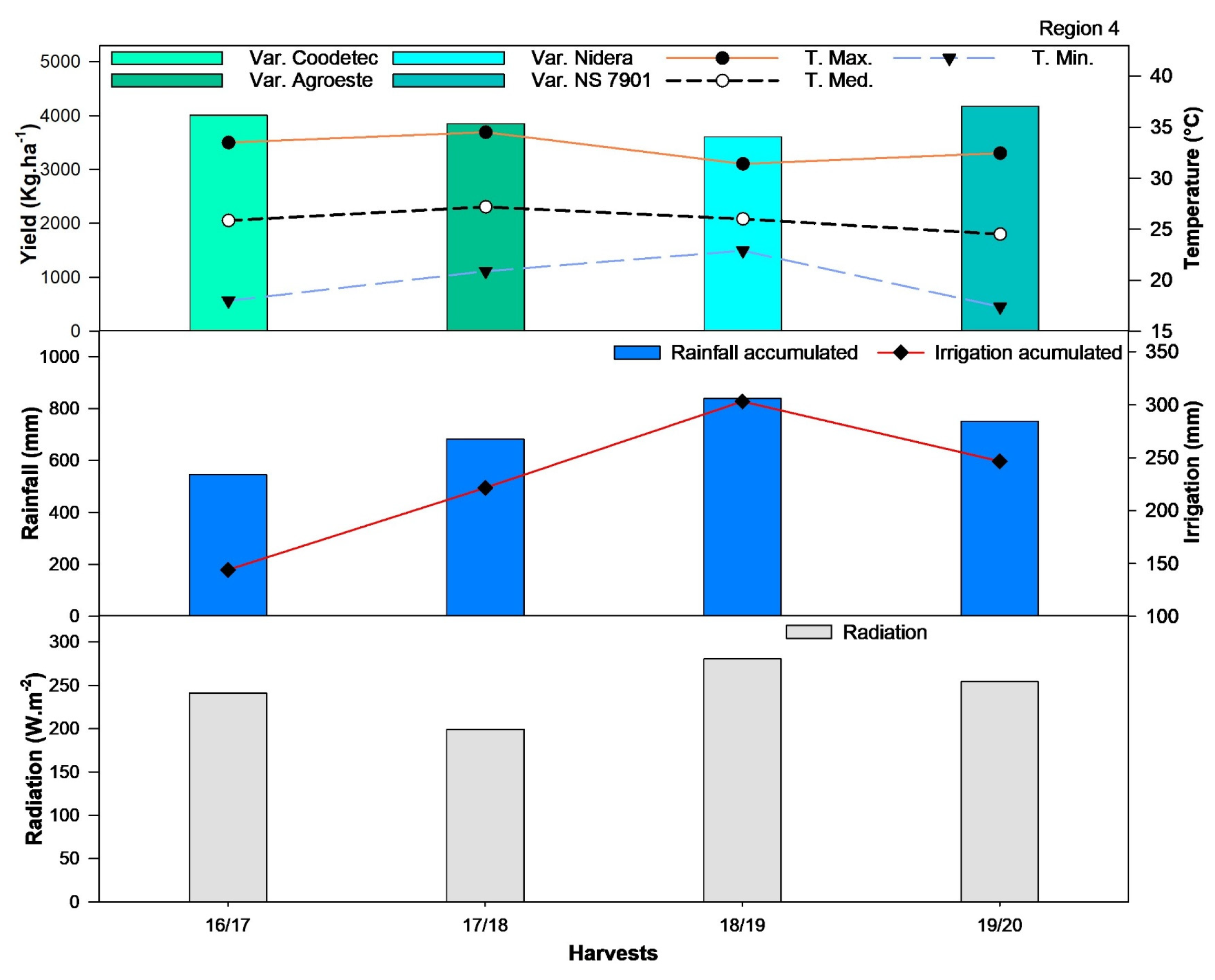
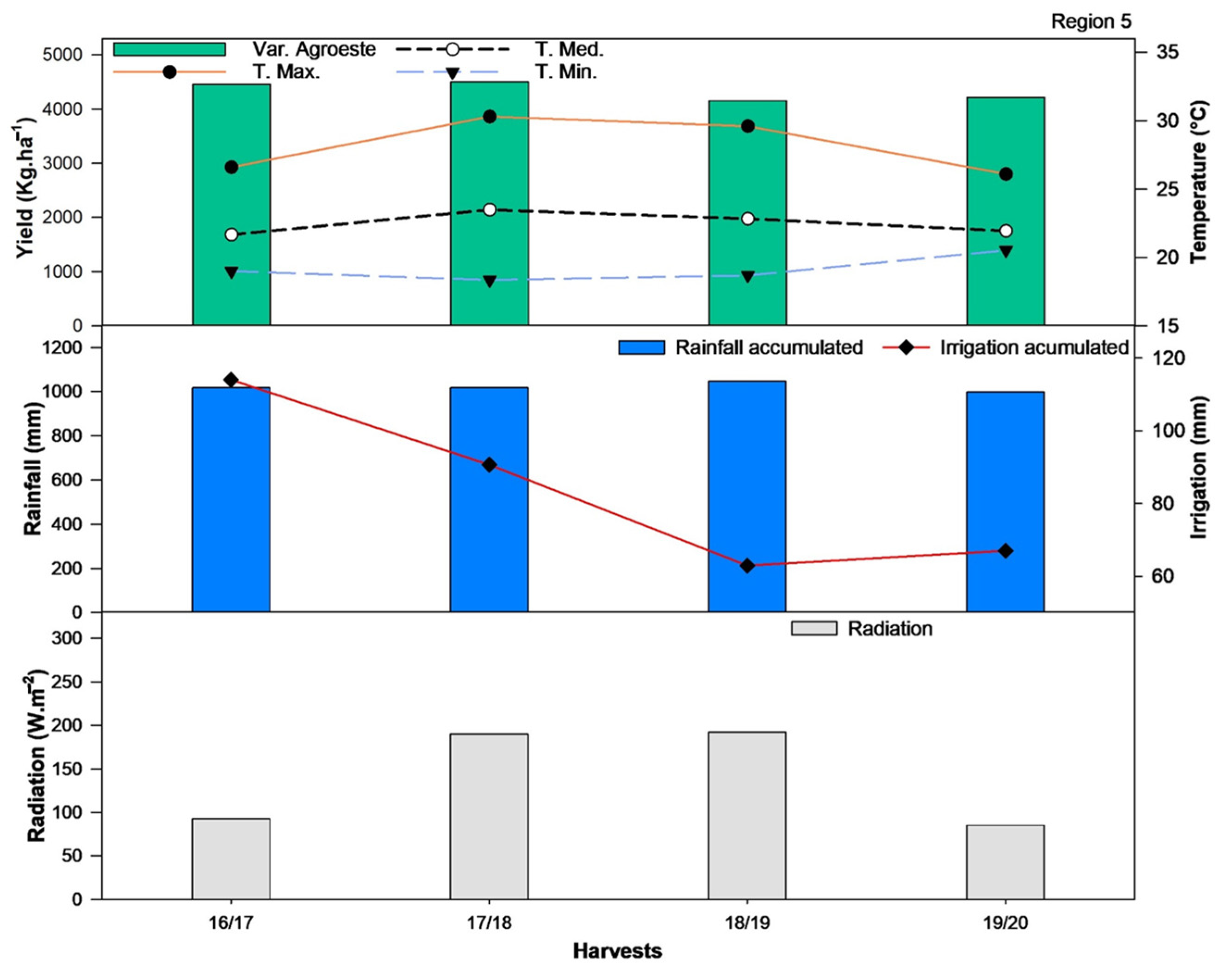
3. Results
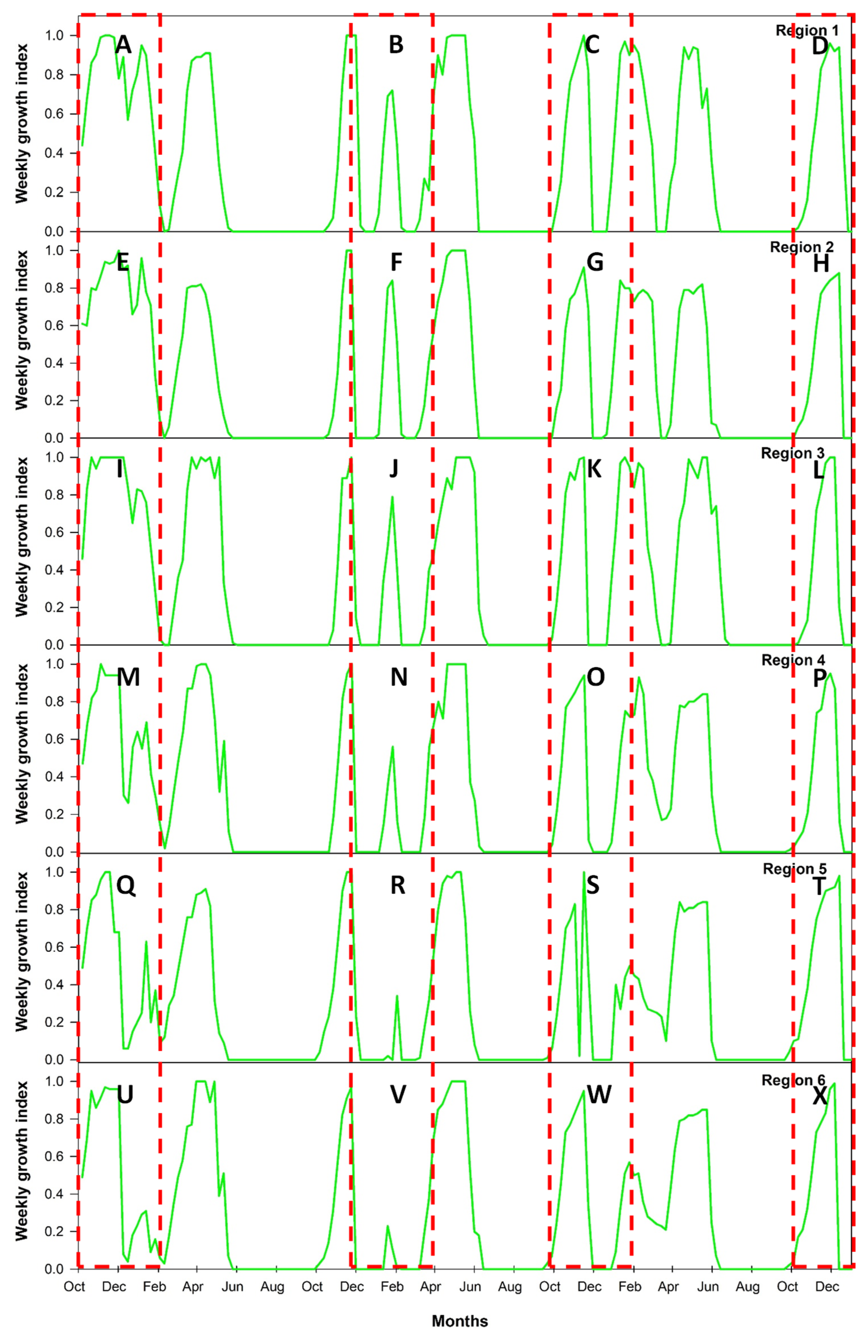
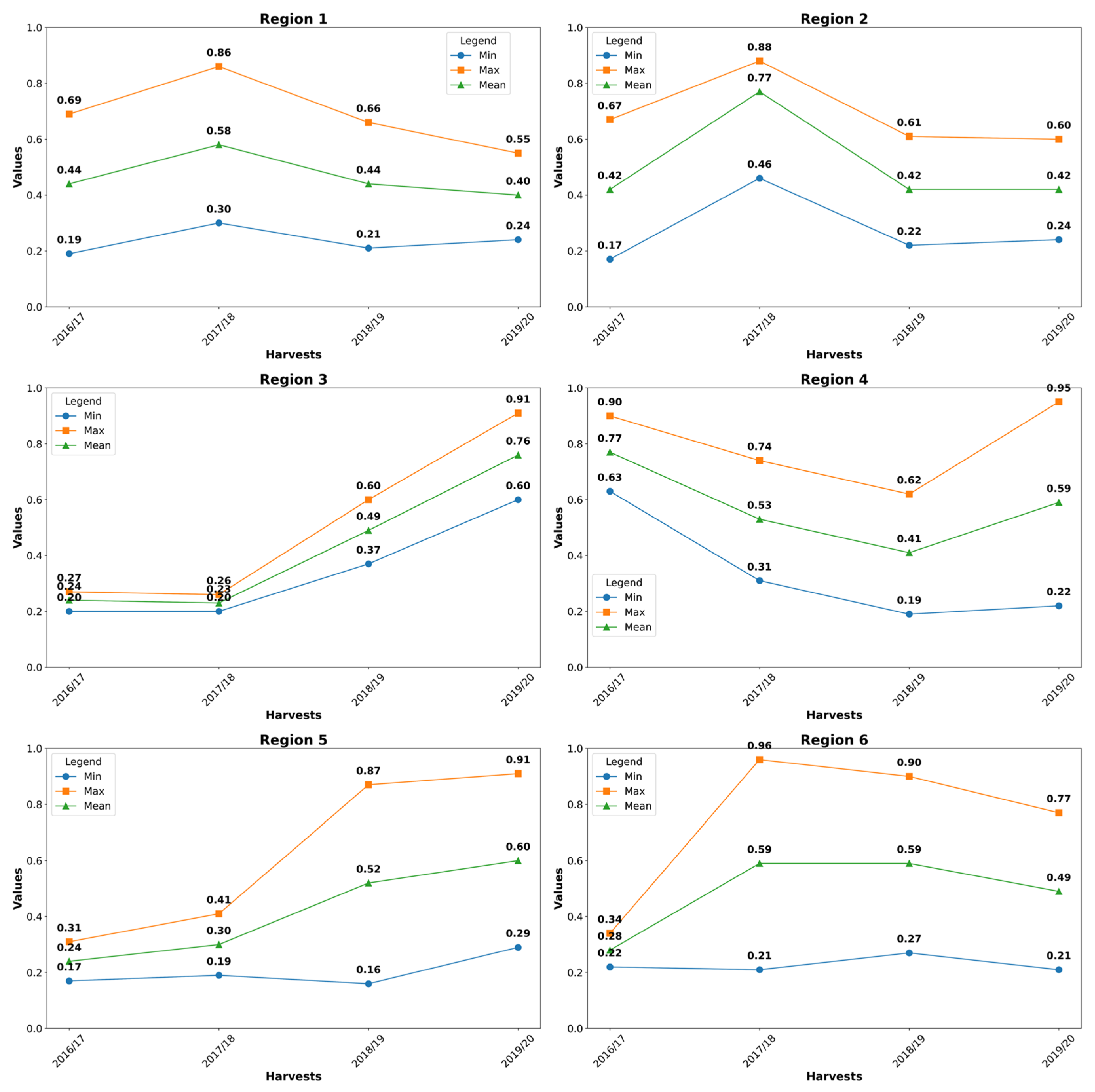
3.1. Growth Indices
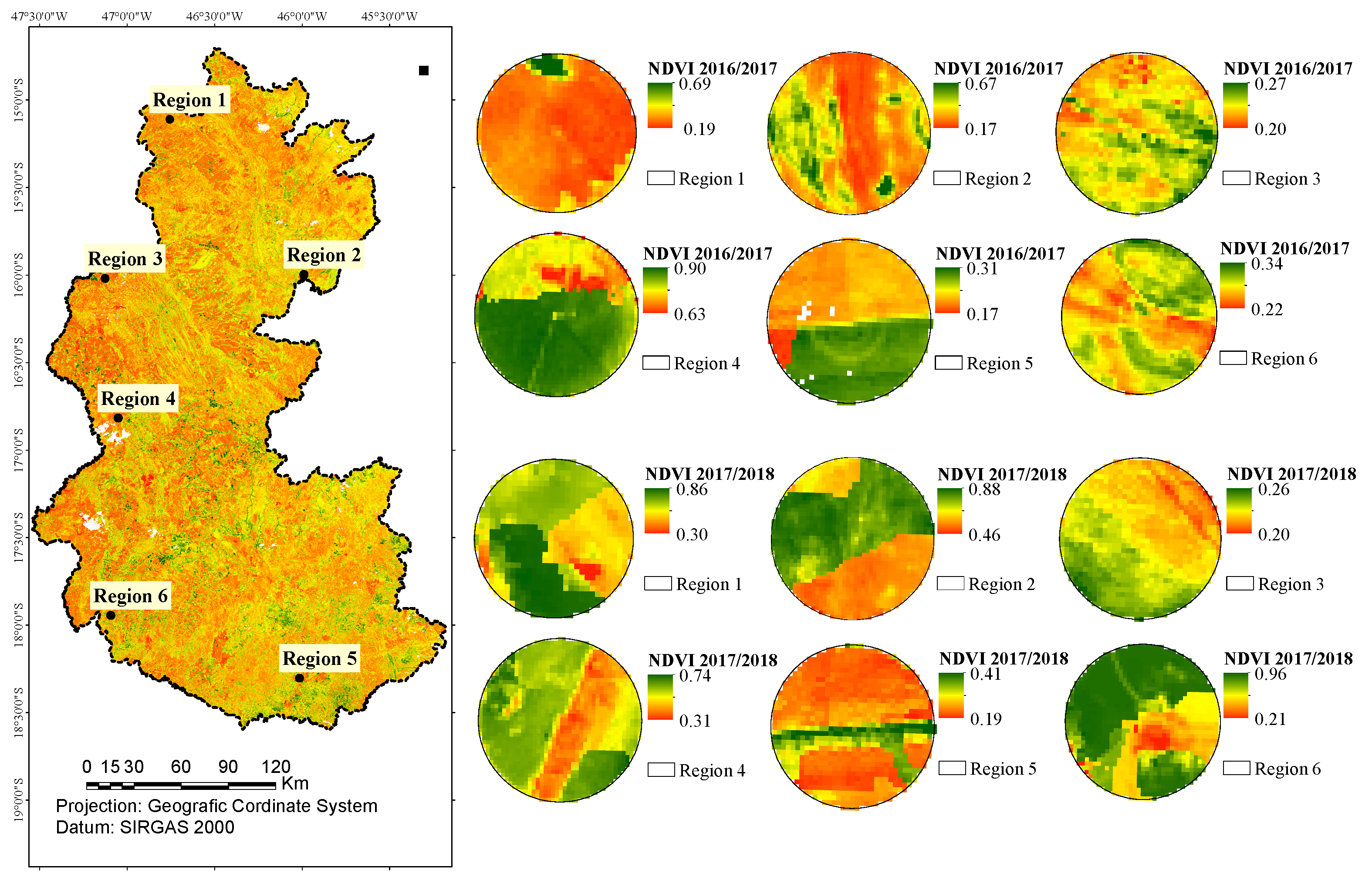
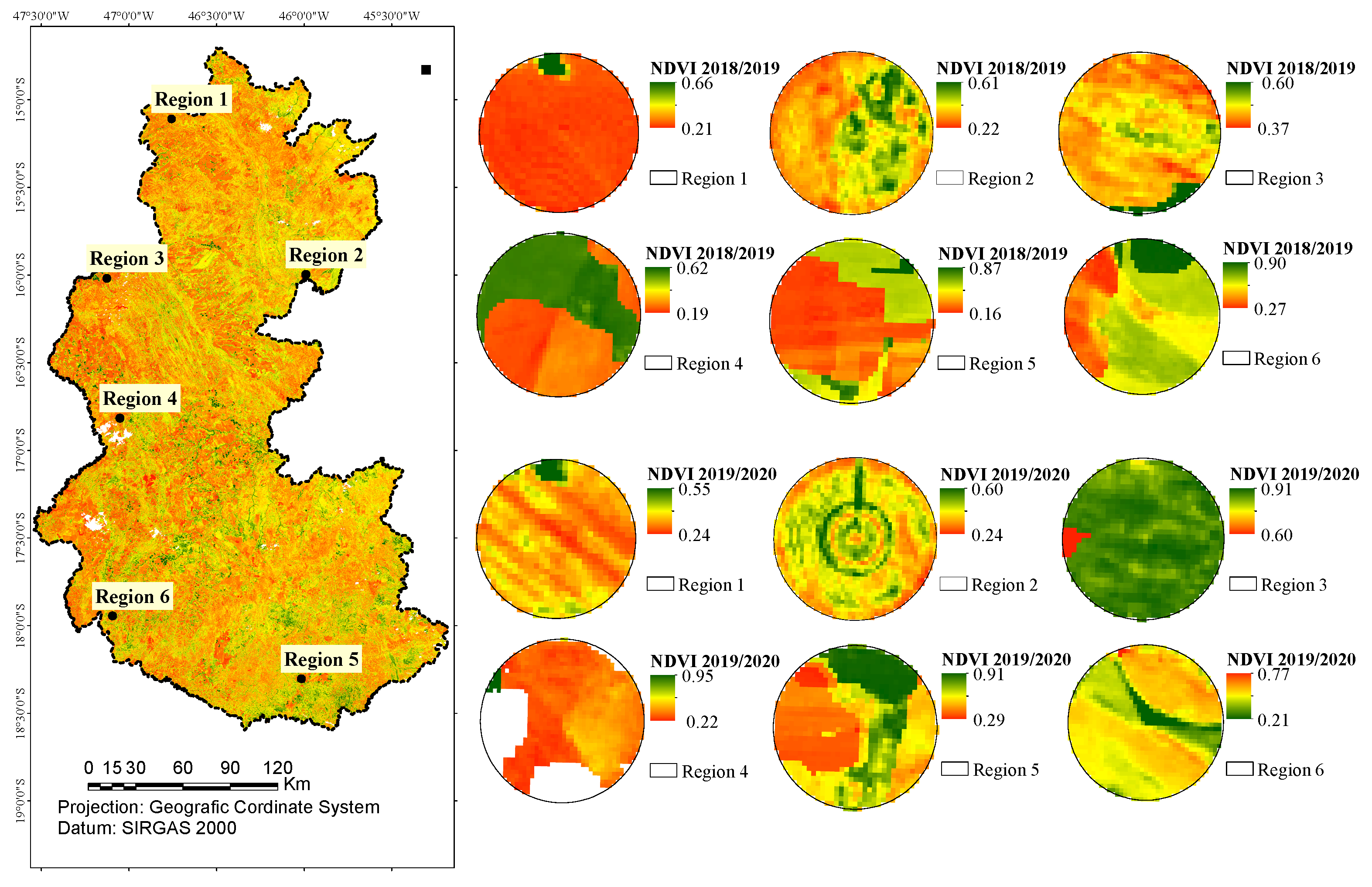
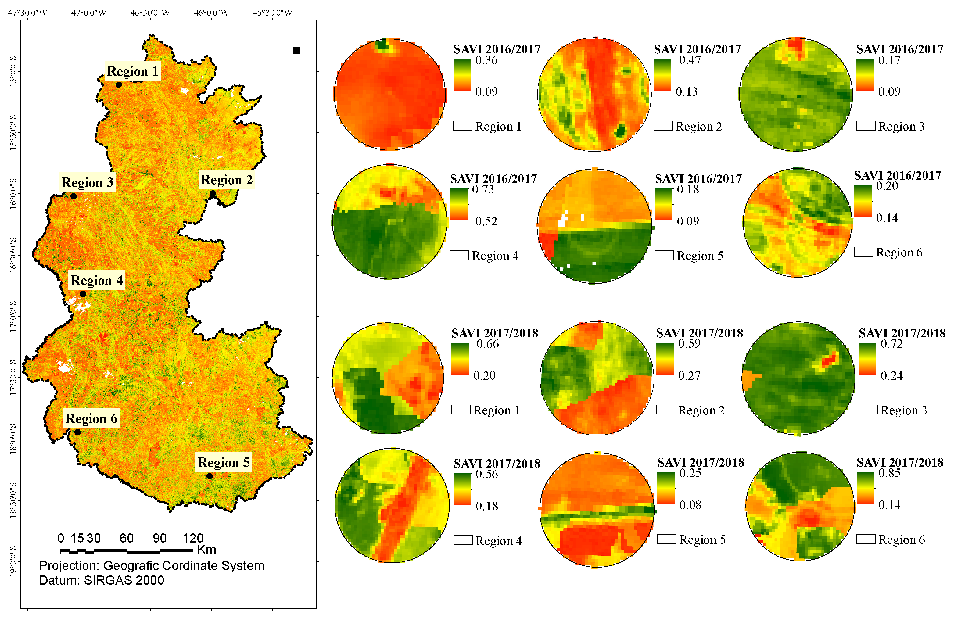
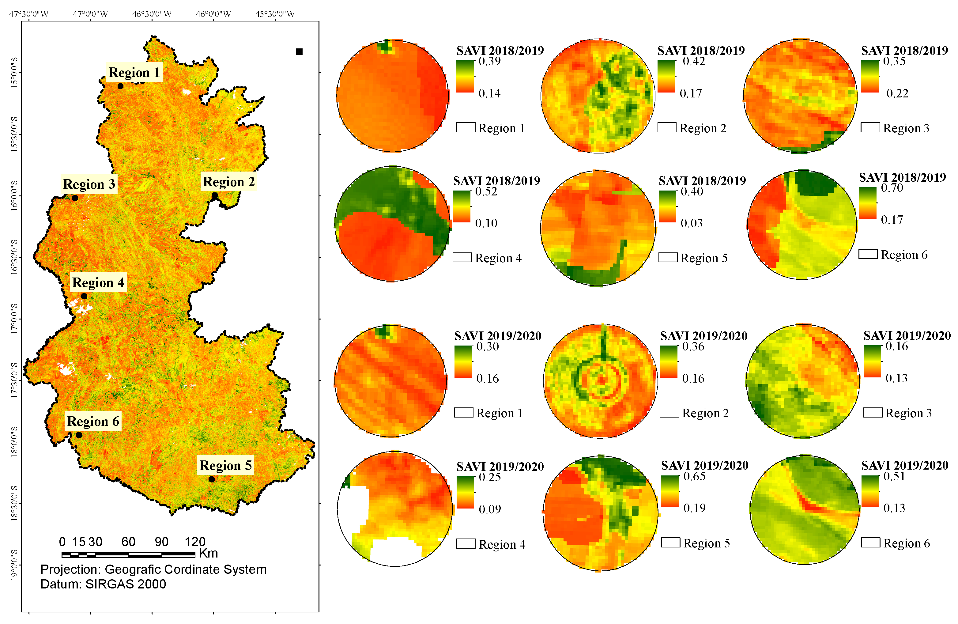
3.2. Vegetation Indices
3.3. Correlation Between Vegetation Indices and Growth Indices
3.4. Soybean Cultivation Data
4. Discussion
5. Conclusions
Author Contributions
Funding
Data Availability Statement
Acknowledgments
Conflicts of Interest
References
- Li, M.-W.; Wang, Z.; Jiang, B.; Kaga, A.; Wong, F.-L.; Zhang, G.; Han, T.; Chung, G.; Nguyen, H.; Lam, H.-M. Impacts of genomic research on soybean improvement in East Asia. Theor. Appl. Genet. 2020, 133, 1655–1678. [Google Scholar] [CrossRef] [PubMed]
- Conab. Acompanhamento da Safra Brasileira 2023/2024-1º Levantamento. 2023. Available online: https://www.conab.gov.br/info-agro/safras/graos/boletim-da-safra-de-graos?start=10 (accessed on 9 April 2024).
- de Oliveira, Z.B.; Knies, A.E.; Bottega, E.L.; da Silva, C.M.; Gomes, J.I.T. Influência da irrigação suplementar na produtividade de cultivares de soja para a safra e safrinha 2018–19 e 2019–20 na região central do RS. Braz. J. Dev. 2021, 7, 15580–15595. [Google Scholar]
- Marcuzzo, R.I.R. Soja no Rio Grande do Sul: Um Estudo Sobre a Gestão de Custos dos Pequenos Produtores da Microrregião de Guaporé; UNIVATES: Lajeado, Brazil, 2023. [Google Scholar]
- Qiao, C.; Cheng, C.; Ali, T. How climate change and international trade will shape the future global soybean security pattern. J. Clean. Prod. 2023, 422, 138603. [Google Scholar] [CrossRef]
- Jones, J.W.; He, J.; Boote, K.J.; Wilkens, P.; Porter, C.; Hu, Z. Estimating DSSAT cropping system cultivar-specific parameters using Bayesian techniques. Methods Introd. Syst. Models Agric. Res. 2011, 2, 365–393. [Google Scholar]
- Kriticos, D.J.; Maywald, G.F.; Yonow, T.; Zurcher, E.J.; Herrmann, N.I.; Sutherst, R. Exploring the effects of climate on plants, animals and diseases. Climex Version 2015, 4, 184. [Google Scholar]
- Qiao, H.; Feng, X.; Escobar, L.E.; Peterson, A.T.; Soberón, J.; Zhu, G.; Papeş, M. An evaluation of transferability of ecological niche models. Ecography 2019, 42, 521–534. [Google Scholar] [CrossRef]
- Raxworthy, C.J.; Ingram, C.M.; Rabibisoa, N.; Pearson, R.G. Applications of ecological niche modeling for species delimitation: A review and empirical evaluation using day geckos (Phelsuma) from Madagascar. Syst. Biol. 2007, 56, 907–923. [Google Scholar] [CrossRef] [PubMed]
- Regos, A.; Gonçalves, J.; Arenas-Castro, S.; Alcaraz-Segura, D.; Guisan, A.; Honrado, J.P. Mainstreaming remotely sensed ecosystem functioning in ecological niche models. Remote Sens. Ecol. Conserv. 2022, 8, 431–447. [Google Scholar] [CrossRef]
- da Silva, L.R.; Araújo, F.H.V.; Ferreira, S.R.; dos Santos, J.C.B.; de Abreu, C.M.; Siqueira da Silva, R.; Regina da Costa, M. Strawberries in a warming world: Examining the ecological niche of Fragaria×ananassa Duch—Across different climate scenario. J. Berry Res. 2024, 14, 193–208. [Google Scholar] [CrossRef]
- Ferreira, M.L.; Von Dos Santos Veloso, R.; De Oliveira, G.S.; Queiroz, R.B.; Araújo, F.H.V.; De Andrade, A.M.; Da Silva, R.S. Effects of the climate change scenario on Coffea canephora production in Brazil using modeling tools. Trop. Ecol. 2024, 65, 559–571. [Google Scholar] [CrossRef]
- Paterson, R.R.M. Future Climate Effects on Yield and Mortality of Conventional versus Modified Oil Palm in SE Asia. Plants 2023, 12, 2236. [Google Scholar] [CrossRef] [PubMed]
- Litskas, V.D.; Migeon, A.; Navajas, M.; Tixier, M.S.; Stavrinides, M.C. Impacts of climate change on tomato, a notorious pest and its natural enemy: Small scale agriculture at higher risk. Environ. Res. Lett. 2019, 14, 084041. [Google Scholar] [CrossRef]
- Haerani, H.; Apan, A.; Nguyen-Huy, T.; Basnet, B. Modelling future spatial distribution of peanut crops in Australia under climate change scenarios. Geo-Spat. Inf. Sci. 2023, 27, 1585–1604. [Google Scholar] [CrossRef]
- Ramos, R.S.; Kumar, L.; Shabani, F.; da Silva, R.S.; de Araújo, T.A.; Picanço, M.C. Climate model for seasonal variation in Bemisia tabaci using CLIMEX in tomato crops. Int. J. Biometeorol. 2019, 63, 281–291. [Google Scholar] [CrossRef] [PubMed]
- Early, R.; Rwomushana, I.; Chipabika, G.; Day, R. Comparing, evaluating and combining statistical species distribution models and CLIMEX to forecast the distributions of emerging crop pests. Pest Manag. Sci. 2022, 78, 671–683. [Google Scholar] [CrossRef]
- Crosta, A.P. Processamento Digital de Imagens de Sensoriamento Remoto; UNICAMP/Instituto de Geociências: Campinas, Brazil, 1999. [Google Scholar]
- Carvalho, G.C. Uso de Geoprocessamento para Caracterização dos Aspectos Físicos, Uso da Terra e Diagnóstico Ambiental no Município de Campina Do Monte Alegre (SP); UFSCar: São Carlos, Brazil, 2023. [Google Scholar]
- Portz, L.; Guasselli, L.A.; Corrêa, I.C.S. Variação Espacial e Temporal de NDVI na Lagoa do Peixe, RS. Rev. Bras. Geogr. Fís. 2011, 5, 897–908. [Google Scholar]
- dos Santos, H.; de Carvalho Junior, W.; de Dart, R.O.; Áglio, M.; de Souza, J.; Pares, J.; Fontana, A.; Martins, A.d.S.; De Oliveira, A.; Jerônimo Guedes Pares, B.P. O Novo Mapa de Solos do Brasil: Legenda Atualizada; SIDALC: Turrialba, Costa Rica, 2011. [Google Scholar]
- Koeppen, W. Climatologia con un Estudio de los Climas de la Tierra; SIDALC: Turrialba, Costa Rica, 1948. [Google Scholar]
- INMET. Normais Climatológicas do Brasil 1991–2020. Available online: https://portal.inmet.gov.br/uploads/normais/NORMAISCLIMATOLOGICAS.pdf (accessed on 9 April 2024).
- Kriticos, D.; Nitin, K.; Chakravarthy, A.; Swathi, P. Predicting potential global distribution of the black spotted yellow borer, Conogethes punctiferalis Guenée (Crambidae: Lepidoptera) by CLIMEX Modelling. In The Black Spotted, Yellow Borer, Conogethes punctiferalis Guenée and Allied Species; Springer: Berlin/Heidelberg, Germany, 2018. [Google Scholar]
- Ramirez-Cabral, N.Y.Z.; Kumar, L.; Shabani, F. Global alterations in areas of suitability for maize production from climate change and using a mechanistic species distribution model (CLIMEX). Sci. Rep. 2017, 7, 5910. [Google Scholar] [CrossRef]
- Soares, J.R.S.; da Silva, R.S.; Ramos, R.S.; Picanço, M.C. Distribution and invasion risk assessments of Chrysodeixis includens (Walker, [1858]) (Lepidoptera: Noctuidae) using CLIMEX. Int. J. Biometeorol. 2021, 65, 1137–1149. [Google Scholar] [CrossRef]
- Nyamtseren, M.; Pham, T.D.; Vu, T.T.P.; Navaandorj, I.; Shoyama, K. Mapping Vegetation Changes in Mongolian Grasslands (1990–2024) Using Landsat Data and Advanced Machine Learning Algorithm. Remote Sens. 2025, 17, 400. [Google Scholar] [CrossRef]
- Radočaj, D.; Jurišić, M. GIS-Based Cropland Suitability Prediction Using Machine Learning: A Novel Approach to Sustainable Agricultural Production. Agronomy 2022, 12, 2210. [Google Scholar] [CrossRef]
- Morisio, M.; Noris, E.; Pagliarani, C.; Pavone, S.; Moine, A.; Doumet, J.; Ardito, L. Characterization of Hazelnut Trees in Open Field Through High-Resolution UAV-Based Imagery and Vegetation Indices. Sensors 2025, 25, 288. [Google Scholar] [CrossRef]
- Huete, A.R. A soil-adjusted vegetation index (SAVI). Remote Sens. Environ. 1988, 25, 295–309. [Google Scholar] [CrossRef]
- Pearson, K. Notes on the history of correlation. Biometrika 1920, 13, 25–45. [Google Scholar] [CrossRef]
- Shapiro, S.S.; Wilk, M.B. An analysis of variance test for normality (complete samples). Biometrika 1965, 52, 591–611. [Google Scholar] [CrossRef]
- Hopkins, W.G. Correlation Coefficient: A New View of Statistics. Recuper. Available online: http://www.sport.org/resour./stats/correl.html (accessed on 9 June 2024).
- Vozhegova, R.; Likhovid, P.; Lavrenko, S. Vzaiemozviazok mizh normalizovanym dyferentsiinym vegetatsiynym indeksom i zelenym pokryvom u zernobobovykh kultur. In Tekhniko-Tekhnolohichni Aspekty Rozvytku Ta Vyprobuvannia Novoi Tekhniky I Tekhnolohii Dlia Silskohospodarstva Ukrainy; Ukrainian Scientific Research Institute for Forecasting and Testing of Machinery and Technologies for Agricultural Production: Kyiv, Ukraine, 2022; pp. 91–97. Available online: http://tta.org.ua/article/view/264805 (accessed on 9 July 2024).
- Conab. Acompanhamento da Safra Brasileira de Cana-de-Açúcar Safra 2017/18; Conab: São Paulo, Brazil, 2018. [Google Scholar]
- Dalla Rosa, G. Efeito do Fenômeno Enos Sobre a Produtividade de Soja no Brasil; UFFS: Chapecó, Brazil, 2019. [Google Scholar]
- United States. National Weather Service. Office of Science and Technology Integration. Climate Prediction S&T Digest: NWS Science & Technology Infusion Climate Bulletin Supplement; United States. National Weather Service. Office of Science and Technology Integration: Silver Spring, MD, USA, 2019. [Google Scholar] [CrossRef]
- Embrapa. Tecnologias de Produção de soja—Região Central do Brasil 2014; Embrapa Soja: Londrina, Brazil, 2013; Available online: https://www.embrapa.br/busca-de-publicacoes/-/publicacao/975595/tecnologias-de-producao-de-soja---regiao-central-do-brasil-2014 (accessed on 25 April 2024).
- Soares, J.R.S.; Ramos, R.S.; da Silva, R.S.; Neves, D.V.C.; Picanço, M.C. Climate change impact assessment on worldwide rain fed soybean based on species distribution models. Trop. Ecol. 2021, 62, 612–625. [Google Scholar] [CrossRef]
- Wahballah, W.A.; Eltohamy, F.; Bazan, T.M. Influence of attitude parameters on image quality of very high-resolution satellite telescopes. IEEE Trans. Aerosp. Electron. Syst. 2020, 57, 1177–1183. [Google Scholar] [CrossRef]
- Crusiol, L.G.T.; de Fátima Corrêa Carvalho, J.; Sibaldelli, R.N.R.; Neiverth, W.; do Rio, A.; Ferreira, L.C.; de Oliveira Procópio, S.; Mertz-Henning, L.M.; Nepomuceno, A.L.; Neumaier, N. NDVI variation according to the time of measurement, sampling size, positioning of sensor and water regime in different soybean cultivars. Precis. Agric. 2017, 18, 470–490. [Google Scholar] [CrossRef]
- Shane, A.R. High-Resolution Crop Yield Predictions from Satellite-Generated NDVI Images. Master’s Thesis, Iowa State University, Ames, IA, USA, 2021. [Google Scholar] [CrossRef]
- Gao, X.; Huete, A.R.; Ni, W.; Miura, T. Optical–biophysical relationships of vegetation spectra without background contamination. Remote Sens. Environ. 2000, 74, 609–620. [Google Scholar] [CrossRef]
- Asrar, G.; Fuchs, M.; Kanemasu, E.; Hatfield, J. Estimating absorbed photosynthetic radiation and leaf area index from spectral reflectance in wheat 1. Agron. J. 1984, 76, 300–306. [Google Scholar] [CrossRef]


| Index | Parameter | Values |
|---|---|---|
| Temperature | DV0 = lower threshold | 10 °C |
| DV1 = lower optimum temperature | 15 °C | |
| DV2 = upper optimum temperature | 32 °C | |
| DV3 = upper threshold | 37 °C | |
| Moisture | SM0 = lower soil moisture threshold | 0.1 * |
| SM1 = lower optimum soil moisture | 0.5 * | |
| SM2 = upper optimum soil moisture | 1.3 * | |
| SM3 = upper soil moisture threshold | 1.5 * | |
| Cold stress | TTCS = temperature threshold | 10 °C |
| TTHS = stress accumulation rate | −0.00001 week−1 | |
| Heat stress | TTHS = temperature threshold | 37 °C |
| THHS = stress accumulation rate | 0.001 week−1 | |
| Dry stress | SMDS = soil moisture threshold | 0.1 * |
| HDS = stress accumulation rate | −0.006 week−1 | |
| Wet stress | SMWS = soil moisture threshold | 1.7 * |
| HWS = stress accumulation rate | 0.001 week−1 | |
| Degree days | PDD = degree days per generation | - |
| Correlation Coefficient (R + or −) | Classification |
|---|---|
| 0.0–0.1 | Very low |
| 0.1–0.3 | Low |
| 0.3–0.5 | Moderate |
| 0.5–0.7 | High |
| 0.7–0.9 | Very high |
| 0.9–1.0 | Almost perfect |
| Region | Safra | Minimum Value | Maximum Value | Average Value | Figure |
|---|---|---|---|---|---|
| 1 | 2016/17 | 0 | 1 | 0.82 | Figure 3A |
| 1 | 2017/18 | 0 | 0.99 | 0.37 | Figure 3B |
| 1 | 2018/19 | 0 | 1 | 0.61 | Figure 3C |
| 1 | 2019/20 | 0.16 | 0.89 | 0.58 | Figure 3D |
| 2 | 2016/17 | 0.33 | 1 | 0.8 | Figure 3E |
| 2 | 2017/18 | 0 | 0.97 | 0.37 | Figure 3F |
| 2 | 2018/19 | 0 | 0.91 | 0.55 | Figure 3G |
| 2 | 2019/20 | 0 | 0.88 | 0.48 | Figure 3H |
| 3 | 2016/17 | 0.28 | 1 | 0.84 | Figure 3I |
| 3 | 2017/18 | 0 | 0.89 | 0.31 | Figure 3J |
| 3 | 2018/19 | 0 | 1 | 0.6 | Figure 3K |
| 3 | 2019/20 | 0 | 1 | 0.48 | Figure 3L |
| 4 | 2016/17 | 0.26 | 1 | 0.68 | Figure 3M |
| 4 | 2017/18 | 0 | 1 | 0.3 | Figure 3N |
| 4 | 2018/19 | 0 | 0.94 | 0.49 | Figure 3O |
| 4 | 2019/20 | 0 | 0.95 | 0.46 | Figure 3P |
| 5 | 2016/17 | 0.06 | 1 | 0.54 | Figure 3Q |
| 5 | 2017/18 | 0 | 0.98 | 0.24 | Figure 3R |
| 5 | 2018/19 | 0 | 1 | 0.37 | Figure 3S |
| 5 | 2019/20 | 0 | 0.98 | 0.57 | Figure 3T |
| 6 | 2016/17 | 0.04 | 0.97 | 0.54 | Figure 3U |
| 6 | 2017/18 | 0 | 0.94 | 0.25 | Figure 3V |
| 6 | 2018/19 | 0 | 0.95 | 0.95 | Figure 3W |
| 6 | 2019/20 | 0 | 0.99 | 0.47 | Figure 3X |
Disclaimer/Publisher’s Note: The statements, opinions and data contained in all publications are solely those of the individual author(s) and contributor(s) and not of MDPI and/or the editor(s). MDPI and/or the editor(s) disclaim responsibility for any injury to people or property resulting from any ideas, methods, instructions or products referred to in the content. |
© 2025 by the authors. Licensee MDPI, Basel, Switzerland. This article is an open access article distributed under the terms and conditions of the Creative Commons Attribution (CC BY) license (https://creativecommons.org/licenses/by/4.0/).
Share and Cite
de Oliveira, G.S.; Souza, J.P.S.; Cardozo, É.P.; Pacheco, D.G.; Ferreira, M.L.; Picanço, M.C.; Soares, J.R.S.; Alves, A.M.O.S.; de Andrade, A.M.; da Silva, R.S. Correlation Between the Growth Index and Vegetation Indices for Irrigated Soybeans Using Free Orbital Images. AgriEngineering 2025, 7, 67. https://doi.org/10.3390/agriengineering7030067
de Oliveira GS, Souza JPS, Cardozo ÉP, Pacheco DG, Ferreira ML, Picanço MC, Soares JRS, Alves AMOS, de Andrade AM, da Silva RS. Correlation Between the Growth Index and Vegetation Indices for Irrigated Soybeans Using Free Orbital Images. AgriEngineering. 2025; 7(3):67. https://doi.org/10.3390/agriengineering7030067
Chicago/Turabian Stylede Oliveira, Gildriano Soares, Jackson Paulo Silva Souza, Érica Pereira Cardozo, Dhiego Gonçalves Pacheco, Marinaldo Loures Ferreira, Marcelo Coutinho Picanço, João Rafael Silva Soares, Ana Maria Oliveira Souza Alves, André Medeiros de Andrade, and Ricardo Siqueira da Silva. 2025. "Correlation Between the Growth Index and Vegetation Indices for Irrigated Soybeans Using Free Orbital Images" AgriEngineering 7, no. 3: 67. https://doi.org/10.3390/agriengineering7030067
APA Stylede Oliveira, G. S., Souza, J. P. S., Cardozo, É. P., Pacheco, D. G., Ferreira, M. L., Picanço, M. C., Soares, J. R. S., Alves, A. M. O. S., de Andrade, A. M., & da Silva, R. S. (2025). Correlation Between the Growth Index and Vegetation Indices for Irrigated Soybeans Using Free Orbital Images. AgriEngineering, 7(3), 67. https://doi.org/10.3390/agriengineering7030067