Article

Characterization of Irrigated Rice Cultivation Cycles and Classification in Brazil Using Time Series Similarity and Machine Learning Models with Sentinel Imagery

by
Andre Dalla Bernardina Garcia
1,*,
Ieda Del’Arco Sanches
1,2,†,
Victor Hugo Rohden Prudente
3,* and
Kleber Trabaquini
4
1
Remote Sensing Graduate Program (PGSER), Coordination of Teaching, Research and Extension (COEPE), National Institute for Space Research (INPE), Av. dos Astronautas, 1758, São José dos Campos 12227-010, SP, Brazil
2
Earth Observation and Geoinformatics Division (DIOTG), General Coordination of Earth Science (CG-CT), National Institute for Space Research (INPE), Av. dos Astronautas, 1758, São José dos Campos 12227-010, SP, Brazil
3
School for Environment and Sustainability (SEAS), University of Michigan (UofM), 440 Church St., Ann Arbor, MI 48109, USA
4
Santa Catarina Agricultural Research and Extension Corporation (EPAGRI), Rod. Admar Gonzaga, 1347-Itacorubi, Florianópolis 88034-901, SC, Brazil
*
Authors to whom correspondence should be addressed.
In memoriam.
AgriEngineering 2025, 7(3), 65; https://doi.org/10.3390/agriengineering7030065
Submission received: 30 January 2025 / Revised: 23 February 2025 / Accepted: 27 February 2025 / Published: 4 March 2025

Abstract

:
The mapping and monitoring of rice fields on a large scale using medium and high spatial resolution data (<10 m) is essential for efficient agricultural management and food security. However, challenges such as managing large volumes of data, addressing data gaps, and optimizing available data are key focuses in remote sensing research using automated machine learning models. In this sense, the objective of this study was to propose a pipeline to characterize and classify three different irrigated rice-producing regions in the state of Santa Catarina, Brazil. To achieve this, we used Sentinel-1 Synthetic Aperture Radar (SAR) polarizations and Sentinel-2 optical multispectral spectral bands along with multiple time series indices. The processing of input data and exploratory analysis were performed using a clustering algorithm based on Dynamic Time Warping (DTW), with K-means applied to the time series. For the classification step in the proposed pipeline, we utilized five traditional machine learning models available on the Google Earth Engine platform to determine which had the best performance. We identified four distinct irrigated rice cropping patterns across Santa Catarina, where the northern region favors double cropping, the south predominantly adopts single cropping, and the central region shows both, a flattened single and double cropping. Among the tested classification models, the SVM with Sentinel-1 and Sentinel-2 data yielded the highest accuracy (IoU: 0.807; Dice: 0.885), while CART and GTBoost had the lowest performance. Omission errors were reduced below 10% in most models when using both sensors, but commission errors remained above 15%, especially for patches in which rice fields represent less than 10% of area. These findings highlight the effectiveness of our proposed feature selection and classification pipeline for improving the generalization of irrigated rice mapping in large and diverse regions.

1. Introduction

Rice (Oryza sativa) plays a critical role in global food security, with rice being one of the most important grains alongside wheat and corn. In the 2023/2024 season, global rice production was expected to reach approximately 518 million tons, driven primarily by Asian countries, which contributed nearly 89.9% of this total [1]. Although Brazil ranks 11th globally, it is the only non-Asian country with annual production exceeding 10 million tons, achieving approximately 10.55 million tons in the 2023/2024 season [2]. The vast majority of rice in Brazil is grown under irrigated conditions, with surface irrigation systems playing a vital role in sustaining this production. This predominance of irrigated cultivation areas is crucial for maintaining Brazil’s significant contribution to global rice supplies and also for ensuring the stability and productivity of its internal production.
Mapping and monitoring irrigated rice fields is crucial not only due to rice’s central role in global food security but also for effective water resource management. As rice is a staple food for more than half of the world’s population, its production is highly dependent on a stable water supply, making it particularly vulnerable to climate variability and water scarcity [3]. Climate variability significantly impacts rice cultivation by altering planting schedules and growth phases. Rising temperatures accelerate plant development, shorten high-yield periods, and reduce productivity [4]. Studies in Japan and China show changes in rice phenology, with earlier heading dates and longer growing periods, due to temperature changes [5]. Beyond temperature, factors such as wind speed and solar radiation also influence rice growth, though they remain less studied. These climate-driven changes directly impact farmers’ income, requiring adaptive strategies to manage risks from climate extremes [4]. Water availability is another critical factor, especially in areas that depend on rainfall and reservoirs for irrigation. In Santa Catarina, Brazil, normal climate conditions support rice cultivation, but dry years present great challenges, as droughts during peak water demand phases can severely disrupt growth and reduce yields [6]. Accurate and timely mapping helps optimize water distribution and maintain irrigation systems, especially in regions with limited water resources.
Remote sensing technologies, with their high spatial resolution (less than 1 m) to medium resolution (between 5 and 10 m) and temporal resolution (between 1 and 15 days), offer valuable data for detecting changes in crop conditions, managing water efficiently, and responding to environmental challenges, thus supporting sustainable rice production and enhancing resilience to climate impacts [7]. These technologies have become indispensable for distinguishing rice fields and tracking their growth dynamics throughout the growing season. As noted by Stroppiana et al. [8], remote sensing enables precise monitoring of crop phenology, which is essential for both accurate classification and agricultural management. By capturing key stages of rice development, remote sensing facilitates informed decision-making for farmers and policymakers alike, contributing to improved yields, reduced losses, and enhanced food security on both regional and national scales.
Optical and SAR (Synthetic Aperture Radar) sensors offer complementary strengths for mapping and monitoring irrigated rice fields. Optical sensors, like the Sentinel-2 Multispectral Imager (MSI), are widely used to derive vegetation indices, such as the Normalized Difference Vegetation Index (NDVI), which provide insights into plant health and growth stages but are limited by cloud cover, especially during rainy seasons [9,10]. There are different studies that use optical data to monitor rice fields [3,11]. In contrast, SAR sensors, like those on Sentinel-1, are able to capture backscatter from the rice canopy in almost all weather conditions, allowing for the precise tracking of growth stages despite most atmospheric conditions. SAR data are often challenging to interpret because of speckle noise, which arises from random interference in SAR images resulting from constructive and destructive interactions of radar signals. This distorts pixel values and adds variability to classification efforts, making land cover mapping particularly difficult in agricultural regions [12]. The integration of optical and SAR data has proven highly effective, combining vegetation indices with structural information for more accurate rice field mapping, optimizing water use, and supporting sustainable agriculture. There are different studies that have used different SAR bands (C, X, and L) to monitor rice development [13,14,15], however, due to the freely provided Sentinel-1 data, the majority of the studies are conducted using this band C SAR data.
Although numerous studies on rice mapping exist, most focus on models and approaches at a municipal or micro-regional scale. In the study conducted by Crisóstomo de Castro Filho et al. [16], the authors mapped irrigated rice in southern Brazil, evaluating various deep learning models with Sentinel-1 data. Despite the promising results, the study area was limited to a single municipality (Uruguaiana), making the findings highly specific to that region. Similarly, in another study by de Bem et al. [17], the feasibility of using Sentinel-1 data combined with neural network algorithms for rice mapping in a southern Brazilian region was evaluated. Again, despite good results, the study area was limited to a specific 2500 km2 region, limiting the model’s applicability to larger scales. In a more recent study by Fernandes Filho et al. [18], rice was mapped across three municipalities in different regions of Brazil using the Random Forest algorithm and Sentinel-2 data. While the results were satisfactory, the absence of tests with SAR data and the lack of integration between these data sources may limit the model’s applicability to regions with high cloud cover, shadows, or fog. Moreover, none of these studies evaluated variations in rice cultivation types or included areas large enough to account for the heterogeneity of different cultivation systems, which could constrain the application of these models to more diverse rice field landscapes.
Several studies in the literature report the efficiency of various machine learning models for agricultural data classification [19,20,21], typically applied to specific regions. Guan et al. [22] applied a temporal time series similarity clustering, combined with exploratory data analysis to develop a generalizable classification approach in China, using MODIS data. Another study by Chen et al. [3], also in China, employed a mapping approach, using Sentinel-1 and Sentinel-2 data, for a large area. Their classification results showed the best combination of EVI with the VV and VH polarization bands, achieving a producer accuracy for rice of 76.67% and an overall accuracy of 66.07%. However, their approach involved calculating the maximum value of monthly compositions for Sentinel-2 and the minimum value of biweekly compositions for Sentinel-1, resulting in time series of different lengths between the SAR and optical data.
Traditional remote sensing methods struggle to distinguish rice cropping systems due to variations in spatial resolution, atmospheric conditions, and rice cultivation dynamics [23]. Dynamic Time Warping (DTW) offers a solution by aligning time series data from optical and SAR imagery, enabling robust classification of rice fields across diverse landscapes [24]. It facilitates the identification of rice growth stages, particularly in fragmented agricultural regions where conventional classification methods often struggle. Additionally, DTW enhances satellite-based crop monitoring by compensating for discrepancies in acquisition timing and spatial resolution, improving the reliability of rice field detection. Studies have demonstrated DTW’s high accuracy in differentiating single and multiple cropping systems by comparing NDVI-based growth curves to reference datasets [22]. By computing DTW distances between observed and standard phenology curves, this method quantifies cropping intensity. Integrating DTW with machine learning further refines classification accuracy and offers a scalable framework for large-scale rice mapping.
In this context, the main objective of this study is to characterize and map the patterns of irrigated rice cultivation in three distinct regions of the Santa Catarina state, Brazil, using satellite images from Sentinel-1 and Sentinel-2. Our goal is to provide a suitable pipeline based on exploratory data analysis and feature selection and transformation techniques for the generalization of irrigated rice fields for large-scale mapping in Brazil.
This study was conducted in two main stages. In the first stage, we performed an exploratory analysis to characterize and subdivide the main irrigated rice cultivation cycles in the northern, central, and southern regions of Santa Catarina. This initial phase provided the foundation for selecting the most representative features and phenological periods for the subsequent stage. In the second stage, we carried out the classification of irrigated rice areas using the previously extracted data, evaluating the performance of five machine learning models across the three regions of the state. In addition to model accuracy, we analyzed the relationship between areas classified as rice and non-rice, considering the spatial density of cultivated areas in each sample patch and their distribution.
In Section 2, the methods, data, and approaches used in this study are described in detail. In Section 3 and Section 4, we present the results and a discussion of these findings, respectively. Finally, in Section 5, we conclude the article with our discoveries and insights gained throughout the course of this study.

2. Material and Methods
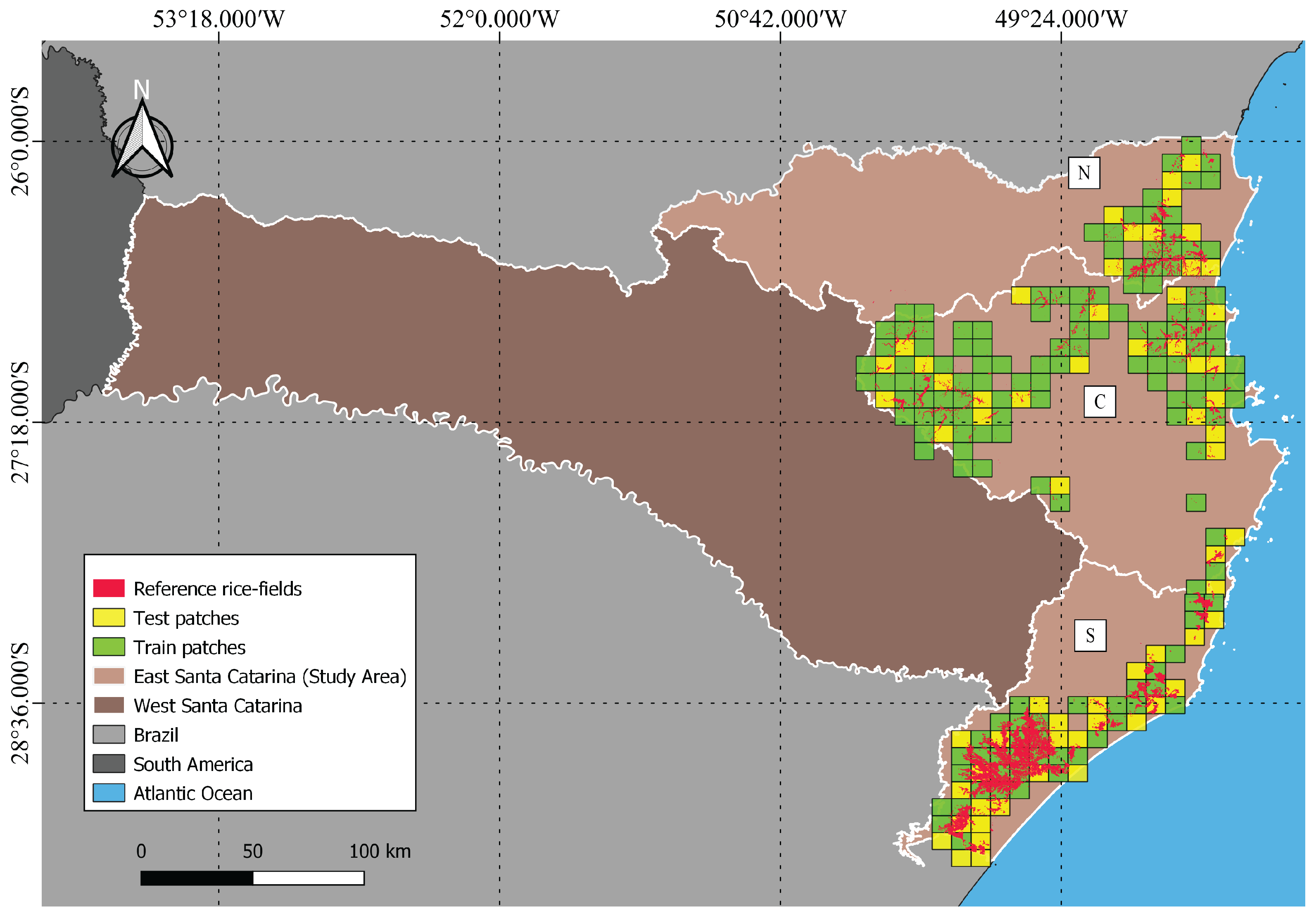
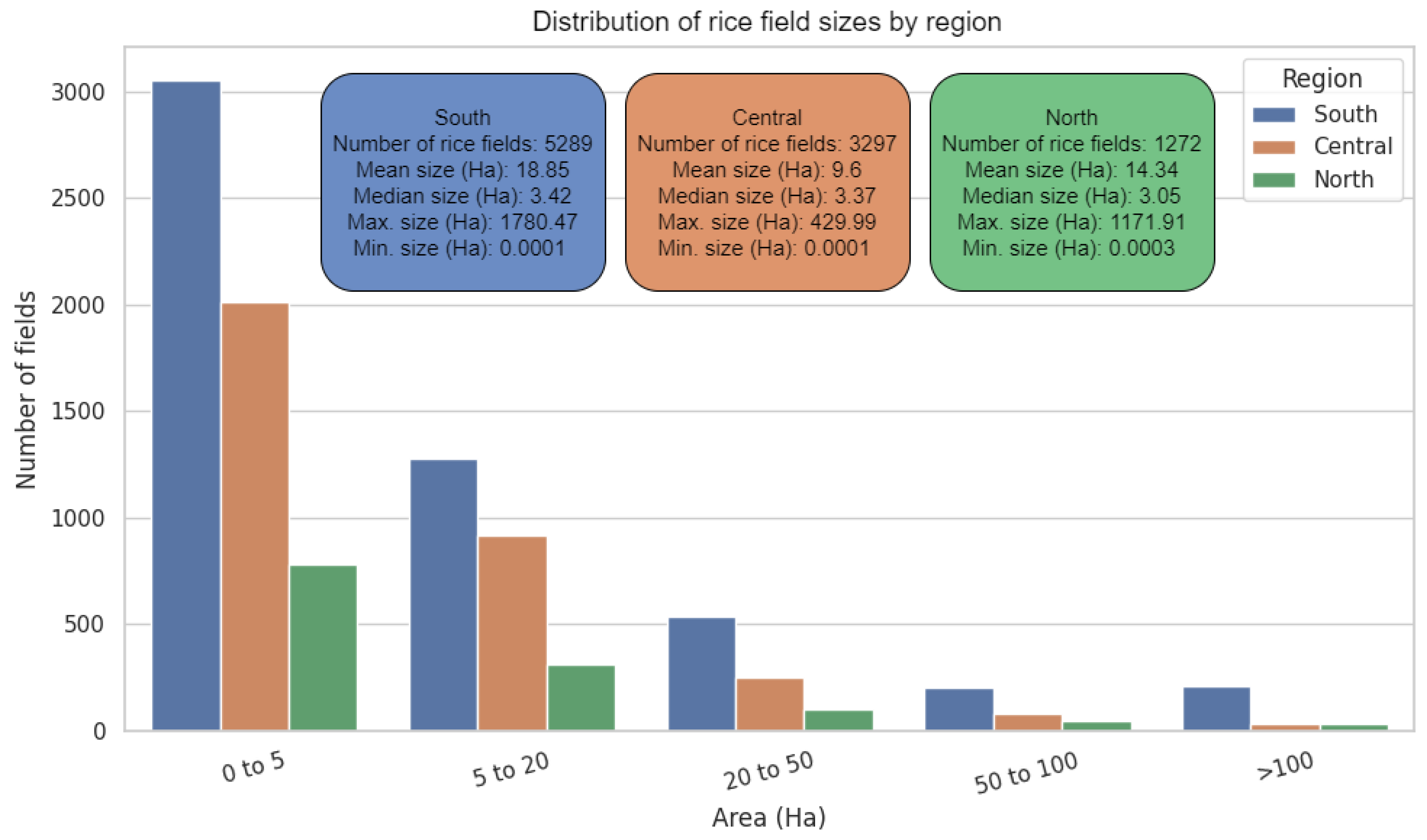
In this section, we describe the study area and detail the acquisition, preparation, integration, and processing of the various data formats. First, we present the study area and their characteristics (Section 2.1). After, in the second topic, Section 2.2, we describe the satellite data and the equations to transform bands and polarization data into vegetation and water indices. In the next topic (Section 2.3), we present the datasets that we used as reference data from irrigated rice fields used for this research. Section 2.4 presents a description of our experimental design, focusing on how we dealt with the high volume data. In Section 2.5, we present the time series clustering methodology. The final section is dedicated to the classification (Section 2.6), focusing on the models and accuracies.

2.1. Study Areas

The Santa Catarina state, Brazil, stands as the country’s second largest rice-producing state, with a total area of 46,008 km2 dedicated to rice fields, distinguished by its diverse topography and climate. Located entirely below the Tropic of Capricorn in the southern hemisphere, the state is bordered by the Paraná state to the north, the Rio Grande do Sul state to the south, Argentina to the west, and the Atlantic Ocean to the east (Figure 1). Spanning approximately 95.7 thousand km2, Santa Catarina is home to about 7.3 million people [25]. The terrain varies significantly, from coastal plains to mountainous areas exceeding 1500 m in elevation, which has a profound impact on the local climate, particularly regarding precipitation and temperature patterns [26].
The irrigated rice cultivation is concentrated in the eastern part of the Santa Catarina state. Due the high heterogeneity in this part, CONAB-Companhia Nacional de Abastecimento [27] and EPAGRI-Empresa de Pesquisa Agropecuária e Extensão Rural de Santa Catarina [28] suggested a division into three primary regions (Figure 1) for irrigated rice cultivation: the north (15.9 thousand km2), the central (2.04 thousand km2), and the south (9.7 thousand km2). This subdivision is based on distinct climate, topography, and agricultural practices. The central and southern regions share a similar cultivation timetable, while the northern region has a shorter growing season (Table 1). Since irrigated rice cultivation is not favorable in the western part, this area was excluded from this study (Figure 1).
The climate in Santa Catarina is classified as humid mesothermal with no dry season and can be further categorized into two subtypes: Cfa, which features hot summers, and Cfb, characterized by mild summers [29]. The central zone, especially the coastal areas and Itajaí Valley, benefits from higher precipitation and temperatures conducive to rice cultivation. The area’s climate is significantly influenced by its topography, with coastal regions receiving increased rainfall due to the orographic effect of nearby mountains [30]. On the other hand, the western part of the central region is characterized by being a high-elevation area, with rice fields located at altitudes of up to 700 to 800 m.
In the northern region, the climate is marked by substantial rainfall, especially during the spring and summer, with annual precipitation exceeding 1750 mm. The area experiences higher average temperatures throughout the year, which supports intensive rice cultivation [6]. The distribution of rainfall provides adequate water for rice crops during critical growth periods, although the region faces drought risks during dry years, making it challenging to maintain optimal water levels for farming.
The southern region, which is the largest rice producer in the state, receives less rainfall compared to the northern and central regions [28]. Summers and springs are particularly dry, with average rainfall ranging between 300 and 450 mm per quarter. Despite this, the region’s climate is generally stable and favorable for rice farming outside the colder months, as low temperatures from May to September can severely impact rice growth. The area’s climatic stability and favorable soil conditions make it ideal for large-scale rice cultivation, though it requires careful water management during dry periods [28].
In the northern region, rice cultivation occurs from August to March. In the central and southern regions, the cultivation extends slightly longer, until April (Table 1). In the south region of Santa Catarina, where the majority of rice fields are located, the management and phenological stages of rice can be divided as follows: Sowing (S) and Emergence (E) occur between August and November, the Vegetative Development (VD) phase takes place between September and December, Flowering (F) typically occurs during the summer between December and January, Grain Filling (GF) occurs from January to February, followed by Maturation (M) and Harvest (H), which can take place from late February to April [27]. Even though Table 1 indicates only a single harvest period, many farmers often conduct a second harvest on the same rice field, making use of the already applied resources like fertilizers, soil preparation, and previously managed efforts [28].
The agricultural system in eastern Santa Catarina is very diverse and is characterized mainly by the production through smallholders. Based on information obtained from reference [31], the region has annual crops such as soy and corn, biennial crops such as cassava, various horticultural species such as lettuce, chives, yerba mate (Ilex paraguariensis), and fruit trees such as banana, viticulture, apple, pear, kiwi, guava, passion fruit, and olives.

2.2. Satellite Data Description and Pre-Processing

This research utilized SAR and optical satellite data from the European Space Agency (ESA). We employed Sentinel-1 (S1), band C, Ground Range Detected (GRD) satellite data for the SAR data (Section 2.2.1). For the optical data, we utilized a Sentinel-2 (S2) Multispectral Instrument (MSI) (Section 2.2.2). In the following subsections, we describe the characteristics, pre-processing, and indices for each of them.
The selection of S1 and S2 satellites was driven by their excellent spatiotemporal coverage and spectral bands ideal for rice monitoring. SAR capabilities ensure reliable data collection even under frequent cloud cover [32], while S2 with 5-day temporal and 10 m spatial resolutions allows for detailed mapping of complex rice field structures [33], surpassing the coarser resolutions of Landsat or MODIS. Furthermore, the free accessibility of their data enhances the feasibility of comprehensive monitoring efforts in the region.

2.2.1. Sentinel-1 GRD

The S1 mission, in Interferometric Wide Swath mode (IW), provides data with ground range usually at 10 m spatial resolution and swath widths greater than 250 km [34]. S1 mission had two satellites in orbit, the Sentinel-1A (S1A) and Sentinel-1B (S1B). More details about the SAR sensor can be found in Table 2.
For this study, we used data from the S1B satellite (referred to as S1 until the end of the paper), since S1A does not cover the entire study area for the specific time windows. S1 GRD data were obtained through the GEE platform, where they are available as pre-processed, ready-to-use images. The pre-processing included applying orbit files, removing border noise, eliminating thermal noise, conducting radiometric calibration, and performing terrain correction using digital elevation models such as the Shuttle Radar Topography Mission (SRTM) 30 m Digital Elevation Model (DEM) or the Advanced Spaceborne Thermal Emission and Reflection Radiometer (ASTER).
Considering that GEE does not automatically implement speckle filtering, which is important for SAR data analysis and classification, additional processing was necessary. Although some researchers suggest using a 7 × 7 window for the Lee filter [12,35], we opted for a 5 × 5 window Lee filter to reduce speckle noise while retaining image details, which is particularly important for the small rice fields (less than 0.5 ha) in our study area. This filter and window size were chosen due to their computational efficiency in the GEE environment and their ability to maintain spatial resolution, as verified by our previous study [36]. Furthermore, a multi-temporal Quegan and Yu filter [37] was applied to enhance temporal consistency throughout the image series. The spatial and temporal domain filters were used with modifications in the scripts provided by [38,39].
The processed S1 GRD data, focusing on VV and VH polarizations, were further used to extract two indices: the Cross-Polarization Ratio (CR) as Equation (1) and the Radar Vegetation Index modified (RVIm) as Equation (2) [40], where σ VH 0 represents the backscatter intensity from VH polarization at the linear scale and σ VV 0 is the backscatter intensity from VV polarization at the linear scale.
CR = σ VH 0 σ VV 0
RVIm = 4 σ VH 0 ( σ VH 0 + σ VV 0 )
We opted to use the CR because it shows a higher correlation with dry biomass compared to individual channels. CR offers better separation of different crops, particularly during the heading and flowering stages [11,41]. Both index-based methods are based on the intensity of backscattering and microwave depolarization. The sensitivity of backscatter intensities to crop phenology and growth morphology is a well-known way to develop crop monitoring strategies based on scattering powers. Consequently, the received waves in co-polarized (VV) and cross-polarized (VH) channels deliver information about a target based on backscatter intensities.

2.2.2. Sentinel-2

The S2 mission, comprising two satellites (A and B) equipped with the MSI sensor, offers a set of 13 spectral bands and a 5-day revisit time. In this study, we utilized only five spectral bands to compute the chosen indices (Table 3). For this study, S2 data were sourced from the “COPERNICUS/S2_HARMONIZED” collection on the GEE platform, which provides Top-of-Atmosphere (TOA) images. Since the harmonized surface reflectance collection started after the study period, we applied the Sensor Invariant Atmospheric Correction (SIAC) algorithm to convert TOA reflectance to Bottom-of-Atmosphere (BOA) reflectance [42]. The SIAC algorithm, supported by the Moderate Resolution Imaging Spectroradiometer (MODIS) and the Copernicus Atmosphere Monitoring Service (CAMS) forecasting system, estimates atmospheric parameters and land surface reflectance to perform atmospheric correction. Detailed information on the SIAC algorithm can be found in Yin et al. [43]. Additionally, cloud and shadow pixels were filtered using a combination of quality bands and cloud shadow masking techniques, based on MAX_CLOUD_PROBABILITY (25%) and CLOUDY_PIXEL_PERCENTAGE (50%) metadata properties of each image contained in the collection.
Given that the MSI SWIR bands possess a spatial resolution of 20 m, we utilized the resampling and reprojection techniques provided by the GEE platform to achieve a 10 m resolution, consistent with the other bands employed. Detailed information on the resampling procedures can be found in the function descriptions within the GEE platform documentation [44].
The study used four different spectral indices derived from the MSI bands. The NDVI (Equation (3)) and the Enhanced Vegetation Index (EVI) (Equation (4)) are commonly used for vegetation analysis. The Normalized Difference Water Index (NDWI) (Equation (5)) and the Modified Normalized Difference Water Index (MNDWI) (Equation (6)) are traditionally used to monitor water bodies, particularly in the context of rice cultivation. These indices were selected based on their effectiveness in detecting vegetation vigor and water presence, which is important to understand the environmental dynamics within the study area.
NDVI = ( ρ NIR ρ red ) ρ NIR + ρ red
EVI = G { ρ NIR ρ red ( ρ NIR + C 1 ( ρ red C 2 ( ρ blue + L ) ) ) }
NDWI = ( ρ green ρ NIR ) ( ρ green + ρ NIR )
MNDWI = ( ρ green ρ SWIR 1 ) ( ρ green + ρ SWIR 1 )
The symbol ρ represents the surface reflectance, with subscripts indicating different spectral bands: ρ N I R for the near infrared, ρ red for the red, ρ blue for the blue, ρ green for the green, and ρ SWIR 1 for the shortwave infrared band. C1 and C2 are aerosol coefficients and have been set at 6 and 7.5, while G is a gain factor (set at 2.5) and L is a canopy background adjustment, set at 1.0, according to most studies reviewed [45,46,47].

2.3. Irrigated Rice Fields Reference Data

The optimal reference data should be ground-truth data. However, there is a lack of such data in Brazil. The few databases available focus on large areas in the central part of the country [48,49,50]. In this sense, as reference data for irrigated rice fields, we used two distinct sources during consecutive crop seasons. The first dataset, covering the 2017/2018 season, was provided by the FlorestaSC research group, a collaborative initiative involving several universities in the Santa Catarina state and the Empresa de Pesquisa Agropecuária e Extensão Rural de Santa Catarina (EPAGRI; Santa Catarina Agricultural Research and Rural Extension Company, Florianopolis, Brazil). The Random Forest (RF) algorithm was used on a series of satellite images to generate this dataset, which achieved a final precision of 95% in 12 categories of thematic land use, including rice fields that were used to produce a binary map. Data integration involved Landsat-8 images, complemented by historical Landsat-5 and Landsat-7 imagery to validate land use and land cover classifications, with computational validation supported by approximately 30,000 verified in situ points [31].
The second reference dataset pertains to the 2018/2019 season and was generated by the Companhia Nacional de Abastecimento (CONAB; National Supply Company, Brasilia, Brazil) and the Agência Nacional de Águas (ANA; National Water Agency, Brasilia, Brazil). This mapping effort focused specifically on irrigated rice areas and was executed using cloud-free Sentinel-2A and 2B image time series. The NDVI compositions derived from these images were visually interpreted by experts, and when available, high-resolution images from Google Earth Pro were used to manually delineate the rice fields. This method ensured a high level of accuracy, with the Kappa index reported at 97% [51].
A 10 m negative buffer was applied to the rice field boundaries in both reference data vector files from the 2017/2018 and 2018/2019 crop seasons. This buffer was introduced to exclude heterogeneous pixels that might result from the inclusion of adjacent materials such as exposed soil, irrigation dikes, and varying vegetation types, as well as different management practices at field borders, as highlighted in the study by Reyes et al. [52]. Following this pre-processing step, the final sampled rice was uploaded to the GEE platform for future analysis.

2.4. Data Preparation and Experimental Design

To better understand the classification of rice fields under different conditions in the state, handle the high volume of data, and speed up processing time in GEE, we divided each region (north, central, and south) into 10 × 10 km patches [53,54]. This grid size was chosen due to GEE’s memory and processing limitations, which were used for data extraction. Larger areas often result in memory overflow errors. Based on this grid, we selected only the patches that contained at least one irrigated rice field.
Next, we performed the annotation process for training and test patches, along with identifying the regions to which they belong. We used data for all the patches for the clustering process. For classification, to ensure effective training and validation of the models (see Section 2.6 for details), 70% of these patches were allocated for training, while the remaining 30% were reserved for testing and validation. A description of the number of patches used can be found in Table 4. This division also plays an important role in understanding the quantity and general dimensions distribution of the rice fields per region (Figure 2).

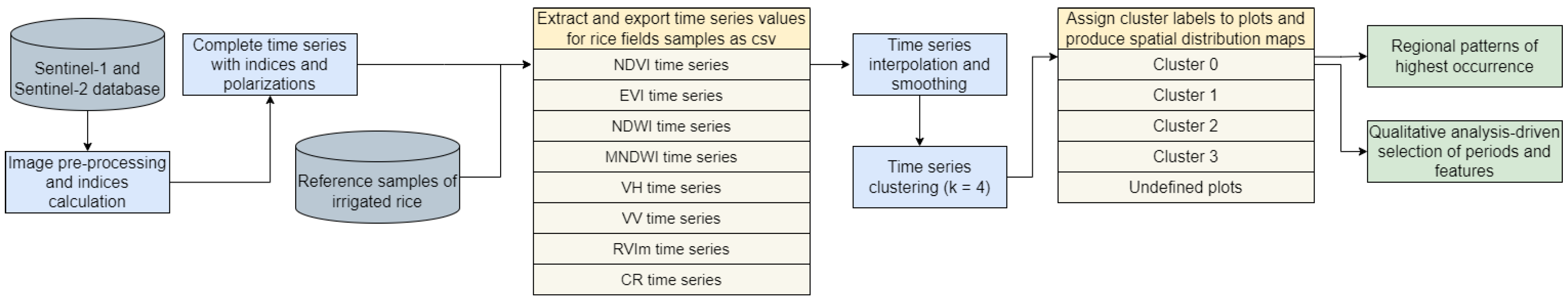
2.5. Time Series Clusterization

To conduct the time series clustering analysis, we first extracted data from all the rice fields in the 154 patches. This involved calculating the mean of specific variables for each individual area on every available date across the two harvest seasons (2017/2018 and 2018/2019). The extracted variables for S1 were VV, VH, CR, and RVIm, and for S2 were NDVI, EVI, NDWI, and MNDWI. After time series data extraction, we removed poor time series (e.g., time series that presented missing or noisy images for some patches) and applied a smoothing process with the Savitzky–Golay filter as obtained from the scipy.signal library through the savgol_filter function. The parameters were defined as window_length = 5 and polyorder = 2. A detailed flowchart outlining the processes used to obtain the most prevalent time series and the distribution map of different crop types by region is presented in Figure 3.
We synchronized the RS data with the crop phenology. Thus, in our framework, Day of Season (DoS) 1 corresponds to the month of July 1st of each growing season, while DoS 365 represents June 30th of the following year. The selection of images tied to specific phenological dates was highlighted by McNairn et al. [55], which emphasizes the importance of synchronizing satellite acquisitions with crop phenology rather than relying solely on Julian dates. This strategy accommodates changes in the growing season due to variations in planting dates and weather conditions, thus optimizing data acquisition and processing efficiency, especially for large study areas.

Transformation and Extraction of Satellite Features

To categorize the various types of rice cultivation observed in the region into a single irrigated rice class, we employed a time series clustering approach. This enabled us to identify essential patterns and significant periods for irrigated rice in the state. Clustering time series data is a powerful method for analyzing time series images and is crucial for identifying crop areas with similar patterns, which helps to recognize different cultivars and management practices in the cultivation of irrigated rice fields. The TSLearn package meets this demand by clustering large amounts of time series data using the “TimeSeriesKMeans” algorithm, an adaptation of traditional k-means for time series [56]. This algorithm organizes time series into clusters based on their similarity, employing iterative steps to allocate data points to clusters and update cluster centers until convergence is achieved. It accommodates various similarity metrics, including Euclidean distance, Dynamic Time Warping (DTW), and soft DTW (soft-DTW). In this section, we describe the algorithm’s parameters, initialization, cluster assignment, updates, and convergence, as detailed by [56].
We used the customizable parameters of TSLearn, including the number of clusters (n_clusters), metric choice (metric), and initialization methods (init). We specifically explored different cluster numbers (4, 5, 6, 9, and 12) using the “softdtw” metric, setting max_iter_barycenter to 100, n_init to 2, and a fixed random state for reproducibility. Based on the experimental analysis, we determined that k = 4 best represented the general cultivation patterns for irrigated rice, considering the spatial distribution, temporal behavior, and information from experts/field agents. Using other values of k resulted in many specific patterns, reinforcing our choice of k = 4 for training the model on generalized data.
For our study, the soft-DTW method (Equation (7)) was applied, where X i and X j signify the two time series being compared. Here, K denotes the path length, w specifies the k t h element in w for the positions i and j, and γ serves as the smoothing factor. This choice is primarily due to its benefits over conventional DTW and Euclidean distance algorithms.
softDTW ( X i , X j ) = γ log k = 1 K e d ( w k ) K γ
As highlighted by Cuturi [57], soft DTW shares similar time and space complexities with DTW, but its compatibility with kernel machines sets it apart, enhancing performance in cluster classification tasks. This compatibility allows soft DTW to better capture complex relationships and non-linearities in the data. Experimental findings [57,58,59] further underscore the superiority of soft DTW, particularly in computing barycenters and clustering time series data. Additionally, soft DTW has shown promise in multistep-ahead time series prediction, making it especially useful in applications where the loss function benefits from the robustness of DTW compared to the more localized nature of Euclidean distance.
After data clustering, we identified the most indicative time series patterns for each index and polarization by region, focusing on two consecutive seasons (2017/2018 and 2018/2019). We analyzed the percentage of area covered by each pattern, aggregating plot areas in three regions and assigning them to four clusters, excluding “undefined” areas due to noise and cloud cover. By grouping time series with similar behavior across both seasons, we identified the most representative mean time series for irrigated rice in each region. For an in-depth explanation of the pre-processing, interpolation, and clusterization processes, please consult the Supplementary Materials, specifically Figures S12–S14.

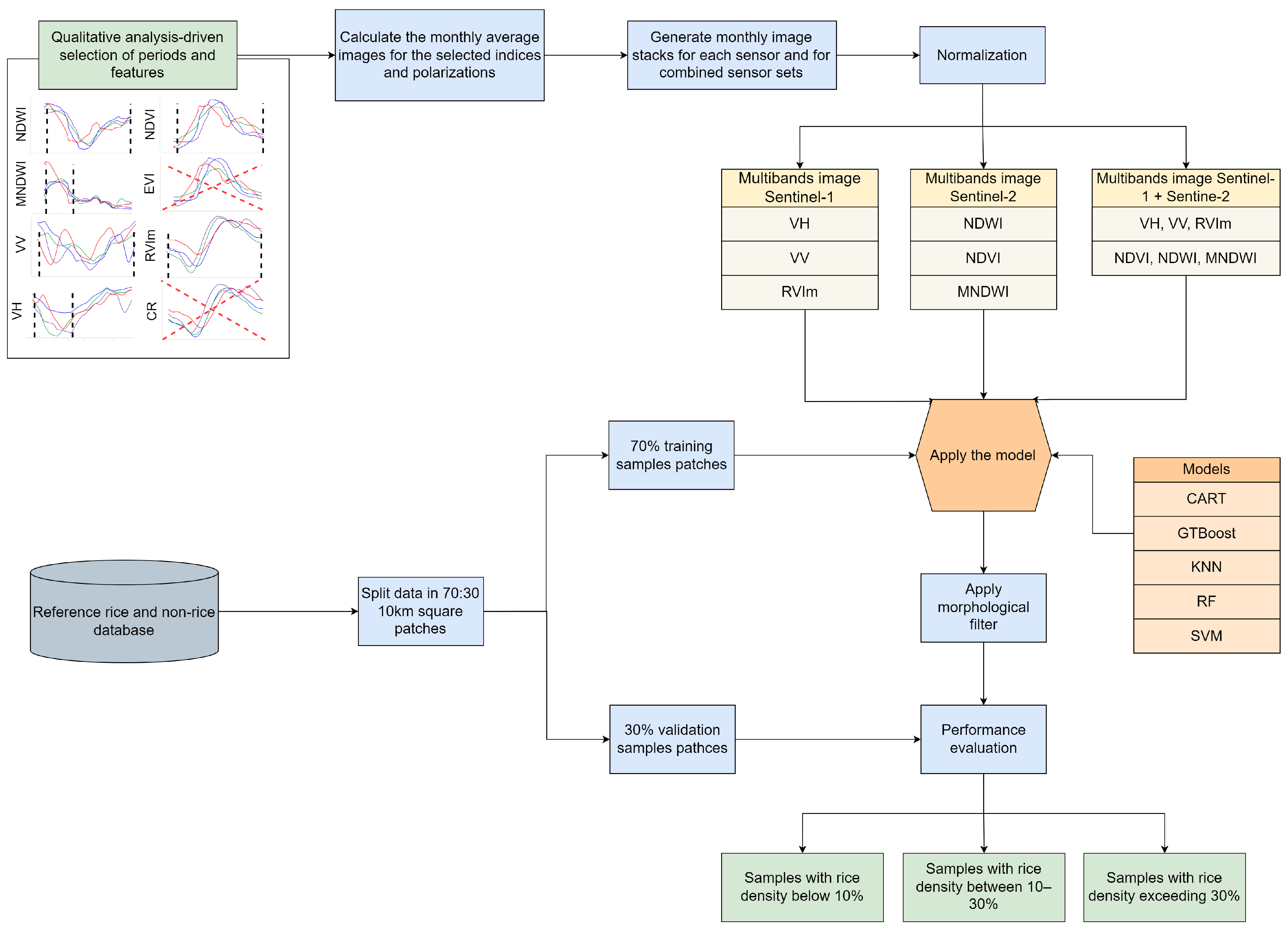
2.6. Rice Classification

After clustering the time series, we moved on to classification. In addition to traditional methods, we introduced an approach that incorporates insights from time series clustering (see Figure 3) as input for classification. Figure 4 presents a detailed flowchart illustrating the processes used to generate binary images distinguishing between irrigated rice and non-irrigated areas. The following subsections detail the data preparation, sample selection, models, and evaluation methods used in this approach.

2.6.1. Satellite Data Preparation

To create a suitable time series for mapping irrigated rice fields across the three macro-regions, we employed a methodology that considered the characteristics of each index and polarization obtained from all training patches, randomly distributed across all study areas. This approach allowed us to generalize the model as efficiently as possible for the entire state. Therefore, particular periods for each polarization and index were chosen to guarantee that the time series captured the key phenological phases of rice growth.
The raw S1 and S2 data are noisy and inconsistent in terms of the number and length of images due to different temporal resolutions, capture dates, cloud cover limitations, etc. To overcome such limitation we used monthly averages, capturing the overall state of each period during the rice crop cycle. This approach reduces variability caused by differences in farmers’ practices, such as soil preparation, planting, irrigation, and harvesting, leading to improved data generalization.
Furthermore, the diversity of rice cultivars and the practice of double harvest in some regions of the state further influence the shape and behavior of the time series curve. These cultivation practices are tied to regional climatic conditions, water availability, and daily sunlight. Therefore, we performed exploratory data analysis to visualize the various types of rice cultivation in the region. This approach was essential in mapping tasks and to explain the final results, as the same indices and polarizations evaluated during exploratory analysis were used for classification. We observed that both VH and MNDWI distinguish themselves during the initial period from late July to late November, while the remaining periods show values more similar to other objects/background. In contrast, NDVI and VV exhibit different and similar values between irrigated rice and other objects throughout the cycle, which led us to use monthly data for the complete series. This approach helped streamline time series processing by reducing the number of images used in the model, focusing only on the indices and time periods that are important for irrigated rice development.
For the VH polarization and for MNDWI, monthly imagery from the beginning of the growing season was utilized. Significant changes in the time series were detected from late July to late November, particularly between days 50 and 160 DoS, due to essential variations occurring during this phase of rice development (for more information see Section 3.1). For the indices, VV, RVIm, NDVI, and NDWI, we used monthly averages throughout the growing season from day 1 to 365 DoS, given the importance of their temporal variation in capturing the unique growth patterns of rice. Consequently, the time series for VV, RVIm, NDVI, and NDWI included 12 monthly images each, while the series for VH and MNDWI comprised 5 images each. The monthly image values were normalized between 0 and 1 to prevent biases arising from the differing value ranges of the radar and optical bands. The CR and EVI indices were excluded from the classification input data, as their time series exhibited similar behavior to RVIm and NDVI, respectively, with slightly lower values. Thus, they provided little to no additional information beyond these two indices.
Finally, a stack or image cube was created using these monthly images and the corresponding index and polarization values. We created three different stacks with the monthly image compositions. The first stack used only S1 (SAR stack) data, and the second stack used only S2 (Optical stack) data. The last stack was a multisensor approach, where we combined the data from SAR and Optical stacks (multisensor stack).

2.6.2. Irrigated Rice Samples

For this step, we used samples from all patches labeled “training”. To avoid class imbalance, which may occur in certain patches, we limited the sample size to 50 points for the target class “irrigated rice fields” and 50 points for the background class “non-irrigated rice”, for each patch. In cases where it was not possible to extract 50 points for each class due to limited rice area, we extracted the maximum possible points for the irrigated rice class and matched the number of points for the non-irrigated rice class. Data from all patches were aggregated into a single dataset for model training (Section 2.6.3). This approach enabled us to extract the values of pixels from all training patches for each satellite data acquisition date (monthly mean; see Section 2.6.1).

2.6.3. Classification Models Training

We selected five classification models: CART, GTBoost, KNN, RF, and SVM. These models were chosen based on their proven success in various studies for classifying different types of crops and other land use and cover targets [20,60,61,62]. Moreover, all of these models are readily available as supervised classification algorithms on the GEE platform.
The CART algorithm is a tree-based model used for both classification and regression tasks. CART constructs a decision tree by recursively splitting the data at each node, aiming to reduce impurity and enhance classification accuracy [62]. The classifier’s strength lies in its ability to create an optimized predictive tree by repeatedly dividing the data until a clear relationship between input and output is established [20]. GTBoost is an ensemble learning algorithm that constructs additive models by sequentially fitting decision trees to the residual errors of previous iterations [63]. GTBoost uses gradient descent to minimize a loss function, effectively reducing prediction errors with each new tree. The resulting model is highly accurate and resilient to overfitting, as the learning rate and other parameters are finely tuned [20]. The KNN algorithm classifies data points based on the majority class among their k-nearest neighbors in the feature space. KNN directly compares each unknown sample against the training data to determine its classification [64]. The simplicity of KNN lies in its reliance on distance metrics, such as Euclidean distance, to identify the closest neighbors. The choice of k, the number of neighbors, is crucial, as a smaller k results in a more complex decision boundary, while a larger k leads to greater generalization [60].
RF is an ensemble-based algorithm that constructs multiple decision trees during training and aggregates their predictions to enhance accuracy and robustness [65]. By creating a collection of trees, RF mitigates the risk of overfitting and improves generalization by averaging the results of individual trees. RF is particularly powerful for handling high-dimensional data and noisy datasets [62]. The SVM is a supervised learning algorithm that constructs a hyperplane to separate data points into different classes. The primary goal of the SVM is to maximize the margin between the classes, ensuring that the nearest data points (support vectors) are as far as possible from the hyperplane. The SVM can handle both linear and non-linear classification tasks by using kernel functions, with the Radial Basis Function (RBF) kernel being particularly effective in capturing non-linear relationships [20]. The choice of parameters such as cost (C) and gamma significantly influences the classifier’s performance, balancing the trade-off between the margin width and misclassification rate [65]. The parameters employed to execute each of the five models are detailed in Table 5.

2.6.4. Classification Evaluation Metrics

To assess the effectiveness of our classification models, we utilized a holistic approach that integrates both qualitative and quantitative evaluations. First, we performed a qualitative analysis to evaluate the models’ capability to distinguish rice fields from other land cover categories. This included assessing the models’ performance in identifying small rice fields and distinguishing rice fields across varying coverage levels in each selected patch: under 10%, from 10% to 30%, and over 30% of the land cover for each 10 × 10 block km2.
For quantitative evaluation, we utilized several metrics derived from the confusion matrix. We calculated the general accuracy, which measures the proportion of correctly classified instances relative to the total number of instances, as defined in Equation (8):
Accuracy = ( TP + TN ) ( TP + TN + FP + FN )
In the context of classifying binary rice maps, True Positive (TP) pixels are those correctly identified as rice, while True Negative (TN) pixels are those correctly identified as non-irrigated rice. False Positive (FP) pixels refer to those incorrectly classified as rice when they are actually non-irrigated rice, and False Negative (FN) pixels are those that were mistakenly classified as non-irrigated rice despite being rice. We also computed precision and recall to provide a deeper understanding of model performance. Precision, which reflects the ratio of true positive predictions to all predicted positives, is calculated using Equation (9) and recall, indicating the proportion of actual positives correctly identified, is determined by Equation (10):
Precision = TP ( TP + FP )
Recall = TP ( TP + FN )
To further evaluate model performance, we employed the Intersection-over-Union (IoU) metric, which is widely used in object detection and segmentation tasks. IoU quantifies the overlap between predicted and actual regions, providing an accuracy measure for the model’s predictions [66]. It is calculated as shown in Equation (11):
IoU = TP ( FP + FN + TP )
For our binary classification task, where 0 represents background and 1 denotes rice fields, we also used the Dice Coefficient to measure the similarity between the predicted segmentation and the reference data. This metric, which assesses pixel-level alignment, is defined in Equation (12) [67]:
Dice = 2 | Y ^ Y | | Y ^ | + | Y |
where Y ^ is the predicted map and Y is the label mask. The Dice Coefficient provides insight into the classifier’s accuracy in identifying rice fields, emphasizing the importance of correctly detecting the target class. In addition, the error of omission (OE) and the commission error (CE) were calculated as Equations (13) and (14), respectively.
OE = 1 - Recall
CE = 1 - Precision

3. Results

Our results are divided into two subsections, highlighting our proposed pipeline to characterize and map the different irrigated rice cultivation patterns in Brazil. The first part, Section 3.1 focuses on the characterization of the regions for each index and polarization, focusing on the most representative time series for each of the three regions by index and polarizations (Section 3.1). This highlights the potential of the DTW algorithm, combined with K-means, to efficiently cluster large datasets over extensive areas. In the second part (Section 3.2), we present the classification results for each model, taking into account the three regions and the proportion of rice fields in each patch sample used.

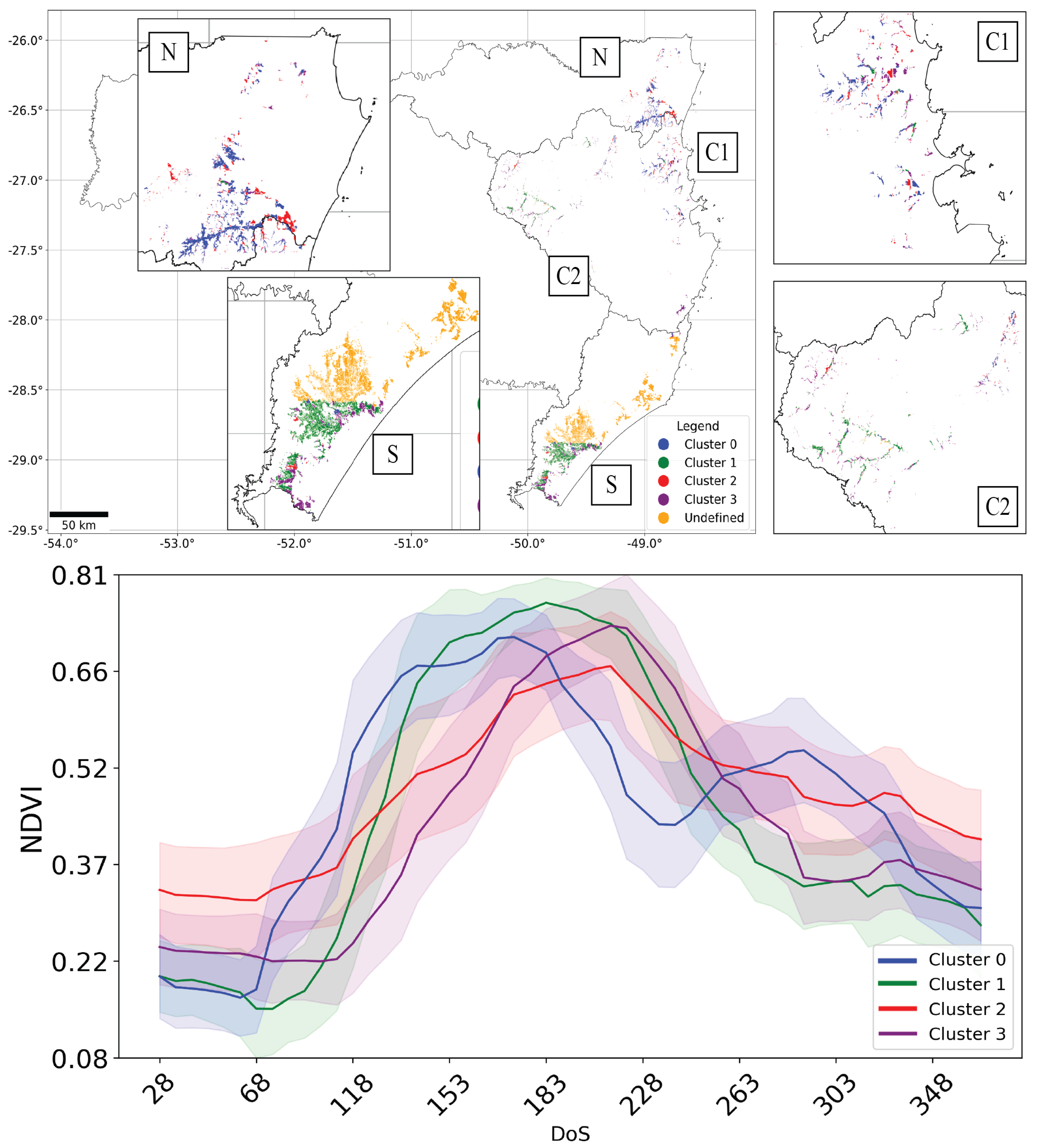
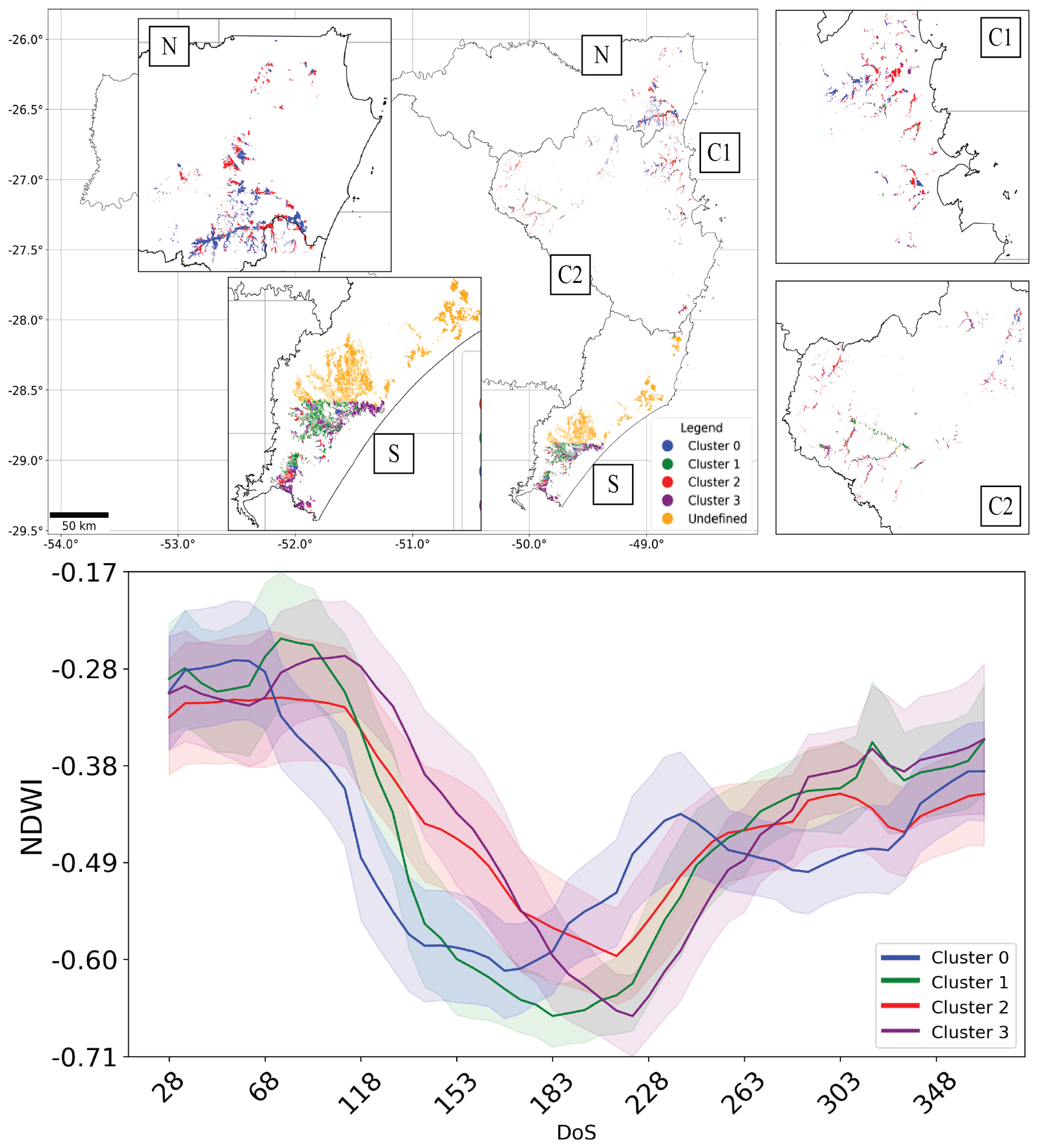
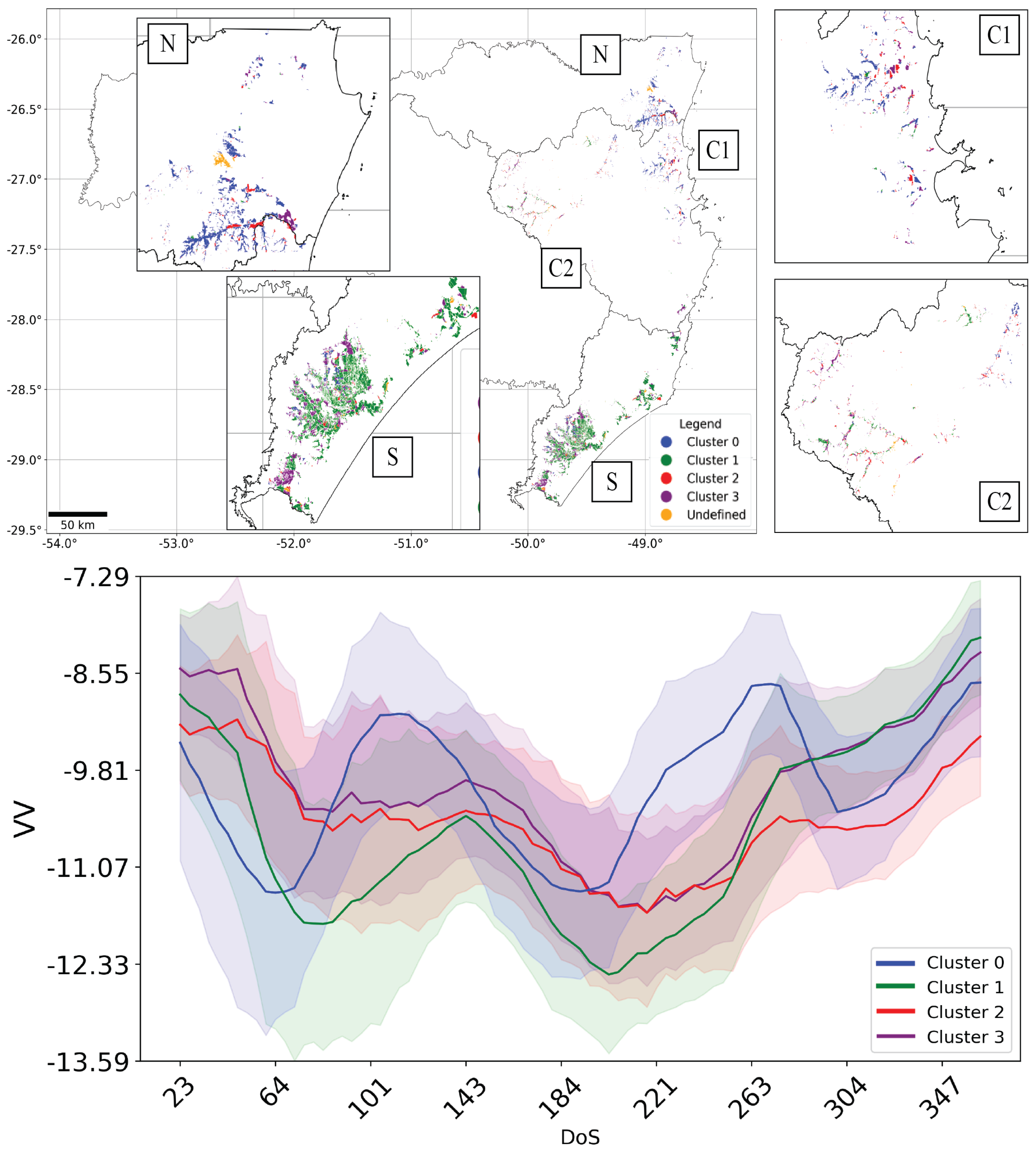
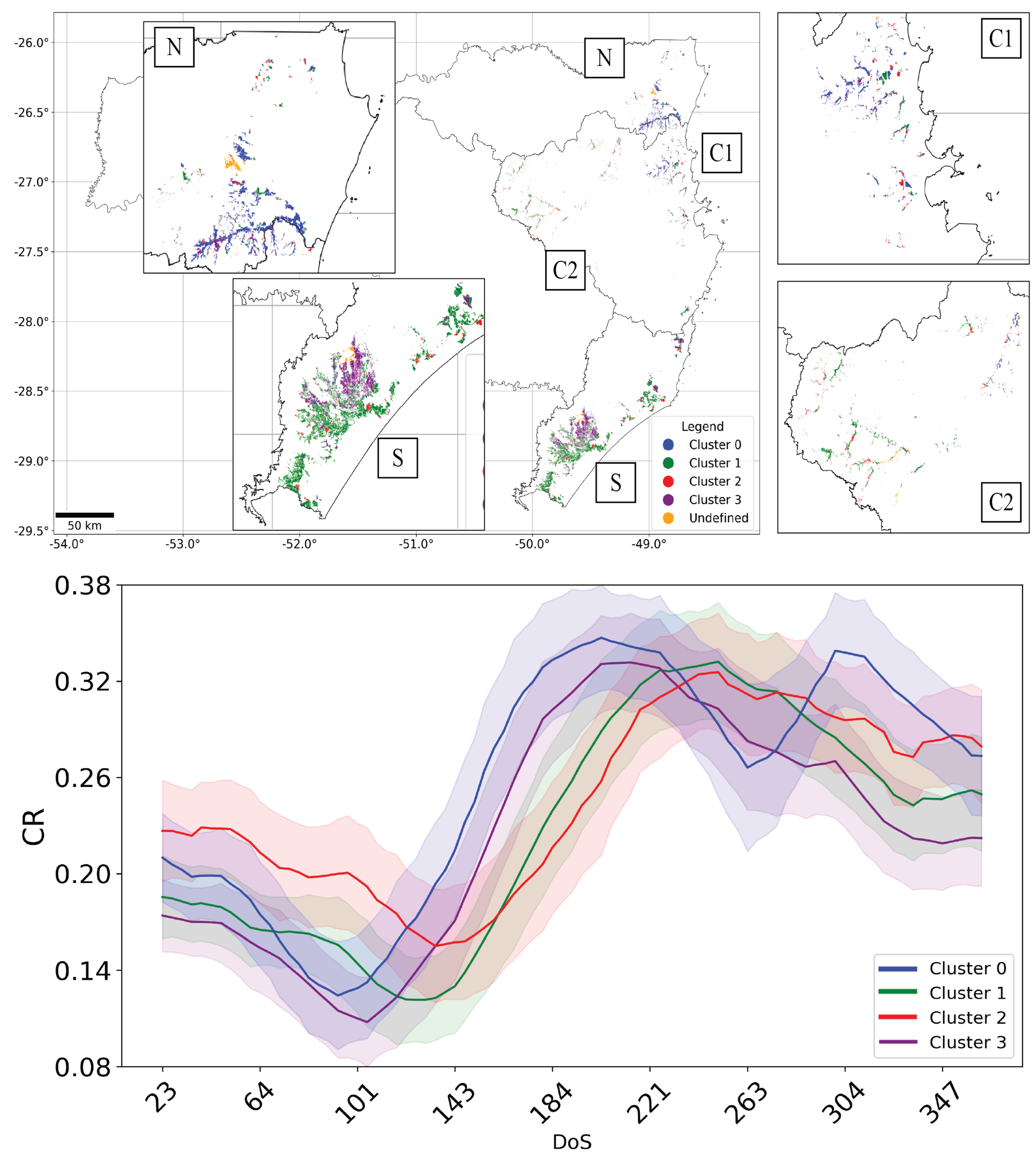
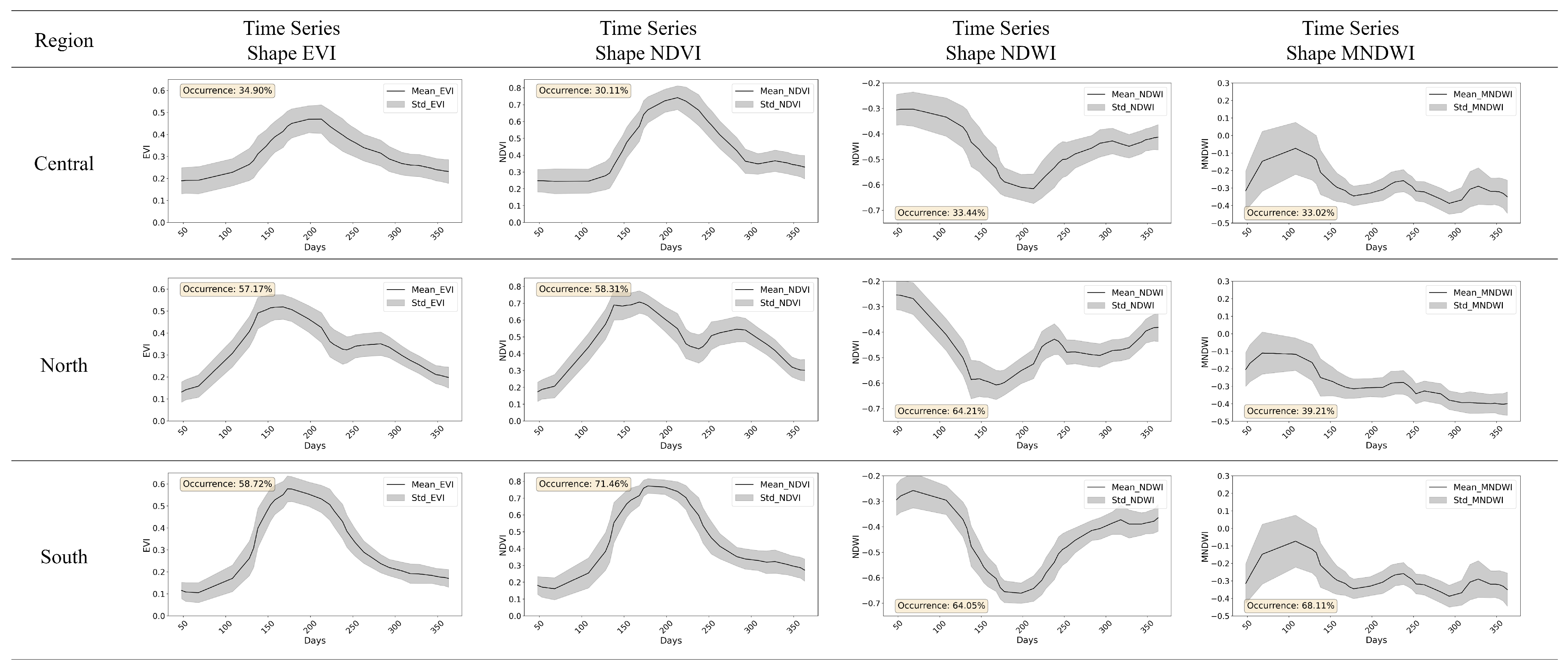
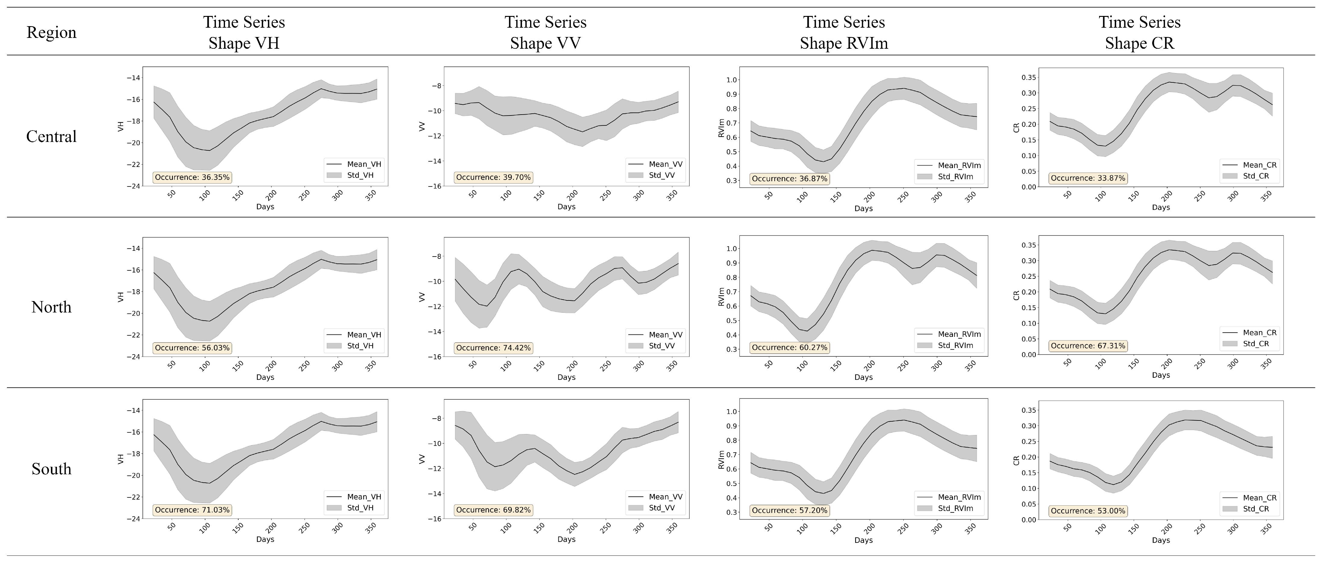
3.1. Exploratory Analysis and Spatial Distribution of Different Irrigated Rice Fields Time Series

The first step in our pipeline is to perform the examination of time series data for irrigated rice fields centered on the efficacy of indices and SAR polarization in distinguishing temporal patterns. Figure 5, Figure 6, Figure 7 and Figure 8 show the spatial distribution of temporal patterns (considering the four clusters) of the NDVI, NDWI, VV and CR, respectively, for irrigated rice fields in the study area. In these Figures, the “undefined” areas correspond to the rice fields that were unclassifiable in terms of cultivation patterns due to the inability to construct a complete time series, either due to cloud cover in optical images or due to excessive noise or missing data in SAR images.
Among these, the NDVI was notable for its robustness in clustering time series with minimal noise and outliers (Figure 5). The NDVI was especially effective in identifying temporal patterns related to rice growth stages, particularly in cases involving multiple harvests or regrowth, as shown in Cluster 0 in Figure 5. The EVI showed behavior similar to that of the NDVI but consistently showed lower values (available in Supplementary Materials Figures S1 and S2, respectively), especially during the peak of vegetative growth. In this research, we found that NDVI values averaged between 0.21 and 0.72 when considering the four clusters.
In terms of the NDWI, the patterns display an inverse relationship to those seen in the NDVI, with the peaks and troughs of the curve appearing in opposite locations (Figure 6). This phenomenon is anticipated because the NDWI in this research indicates the water content within the soil-plant system. Initially, the values are high due to soil preparation and flooding of the rice field to accommodate pre-germinated seeds, with the highest NDWI values for the four clusters averaging between −0.19 and −0.30 (available in Supplementary Materials Figure S3). As the plant growth progresses, the water in the soil–plant system diminishes due to factors such as root absorption, evapotranspiration, and the decrease or cessation of irrigation. Notably, the MNDWI index (available in Supplementary Materials Figure S4) provided critical insights into water content changes within the soil–plant–atmosphere system, particularly during irrigation periods. The most prominent changes were observed between DoS 50 to 150 and from DoS 200 to 250, corresponding to the flooding stage and rainy season, respectively, making this index exceptionally beneficial for monitoring flood events and water management strategies in rice farming.
The VH polarization (available in Supplementary Materials Figure S5) was significantly impacted during the initial phases of the crop season, particularly between DoS 50 and 150, where variations in backscatter intensity were noted due to soil preparation and field flooding. This period was crucial for differentiating flooded rice fields, along with other types of crops in the region such as cassava, as well as horticulture and the cultivation of yerba mate (Ilex paraguariensis), bananas, viticulture, and other fruit crops, even though the data showed some noise. Conversely, VV polarization exhibited more consistent clustering performance over the temporal series (Figure 7 and Supplementary Materials Figure S6), especially in irrigated rice fields double-cropping systems, owing to its interaction with vertically structured crops such as rice, which minimizes signal penetration through the canopy.
The spatial distribution of clusters based on VV polarization revealed distinct patterns among the evaluated irrigated rice fields time series, with noticeable differences between the rice fields and background (non-irrigated rice) throughout the crop season. For instance, as shown in Figure 7, Cluster 2 displayed a flatter curve with less variation in VV values, primarily distributed in the central and northern regions during both crop seasons, while Cluster 1 exhibited more pronounced variation and was dominant across both crop seasons, particularly in the southern region. These spatial patterns underscore the heterogeneity of rice cultivation across the study area and the impact of local agricultural practices on SAR signal response.
The indices Cross-Ratio (CR) (Figure 8 and Supplementary Materials Figure S7) and modified Radar Vegetation Index (RVIm) (Supplementary Materials Figure S8) offered a good alternative to polarizations for clustering crop patterns. The temporal behavior of these indices, especially the sharp drop observed at the end of rice cultivation season (post-260 DoS), was linked to the dynamic changes in VH and VV values due to the rice crop’s phenological development.

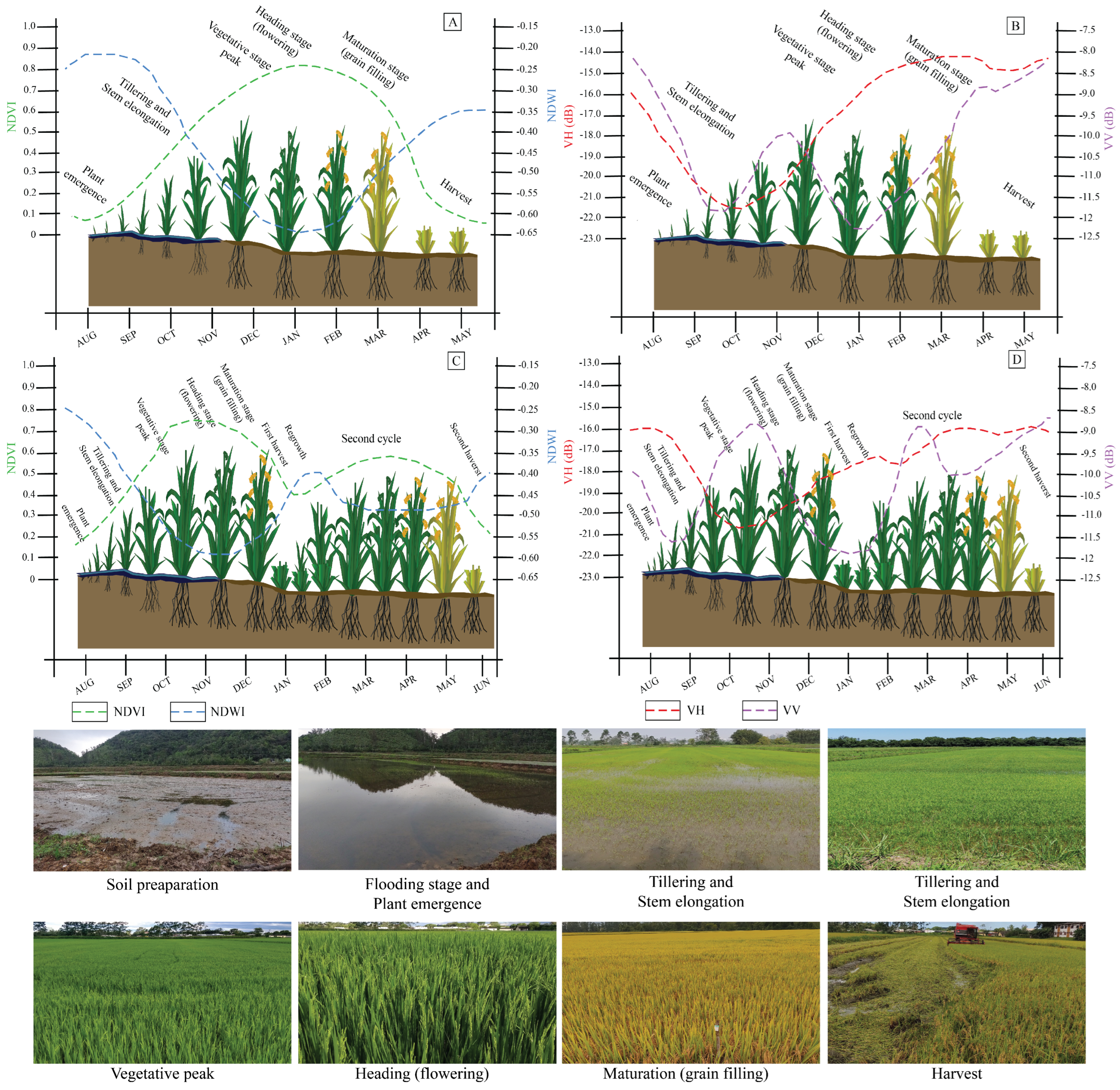
Most Representative Time Series Characterization Results

The optical indices EVI, NDVI, NDWI and MNDWI exhibited specific regional trends. In the northern areas, double cropping was highly prevalent, being represented by over 57% according to these indices (Figure 9). In contrast, single cropping was more typical in the southern regions, starting a bit later, with representativeness between 58% and 71%. The central region, by comparison, showed diminished representativeness across these indices, aligning with its general complexity.
The analysis of optical indices alongside radar data has shown that they provide complementary insights. Optical indices, such as EVI and NDVI, are good at capturing vegetative growth stages, due to the characteristics of red and NIR reflectance bands, with red decreasing and then increasing during ripening, while NIR peaks at heading before declining due to biomass loss. On the other hand, radar data, specifically VV polarization, excels at monitoring alterations in scattering mechanisms resulting from crop development (Figure 10).
The most representative time series of the SAR data for rice fields were determined by averaging data from both seasons, highlighting the most common patterns in the three regions (Figure 10). A widespread temporal pattern was observed in VH polarization throughout all regions, accounting for 36.35% in the central, 56.03% in the north, and 71.03% in the southern regions.
Unlike VH polarization, VV polarization exhibited greater variability (available in Supplementary Materials Figures S5 and S6). Additionally, VV polarization exhibited notable regional differences, with the most frequent behavior covering 74.42% of the northern area and 69.82% of the southern area. Conversely, no single pattern was dominant in the central region, where less than 40% of the area showed the most common behavior. This highlights the complexity of the central region, characterized by variations in altitude, temperature, and precipitation, which complicate rice mapping. The diversity of the central region was linked to its diverse topography, leading to considerable differences in radar acquisition angles.
The RVIm index successfully reflected the relationship between VH and VV polarizations, and its behavior is similar to optical vegetation indices (available in Supplementary Materials Figure S8). It reached the highest value at the peak of volumetric scattering and decreased as the crop advanced in maturity and was harvested. This index is highly useful for observing changes in vegetation biomass and could be an essential instrument for monitoring the growth of rice crops in various regions. The noted variations in SAR signal response throughout different crop stages highlight the need for a multi-index strategy to achieve precise rice field classification (see Supplementary Materials Figures S1–S8).
According to our results, we can use SAR and optical data as complementary datasets. Figure 11 represents an overview of the relationships between SAR and optical data at different rice phenology stages. This indicates that SAR data can serve to bridge the gaps when optical data are missing and vice versa, thereby strengthening the reliability of crop monitoring. Moreover, this relationship between SAR and optical data could be a good source to use as input in the rice classification process.

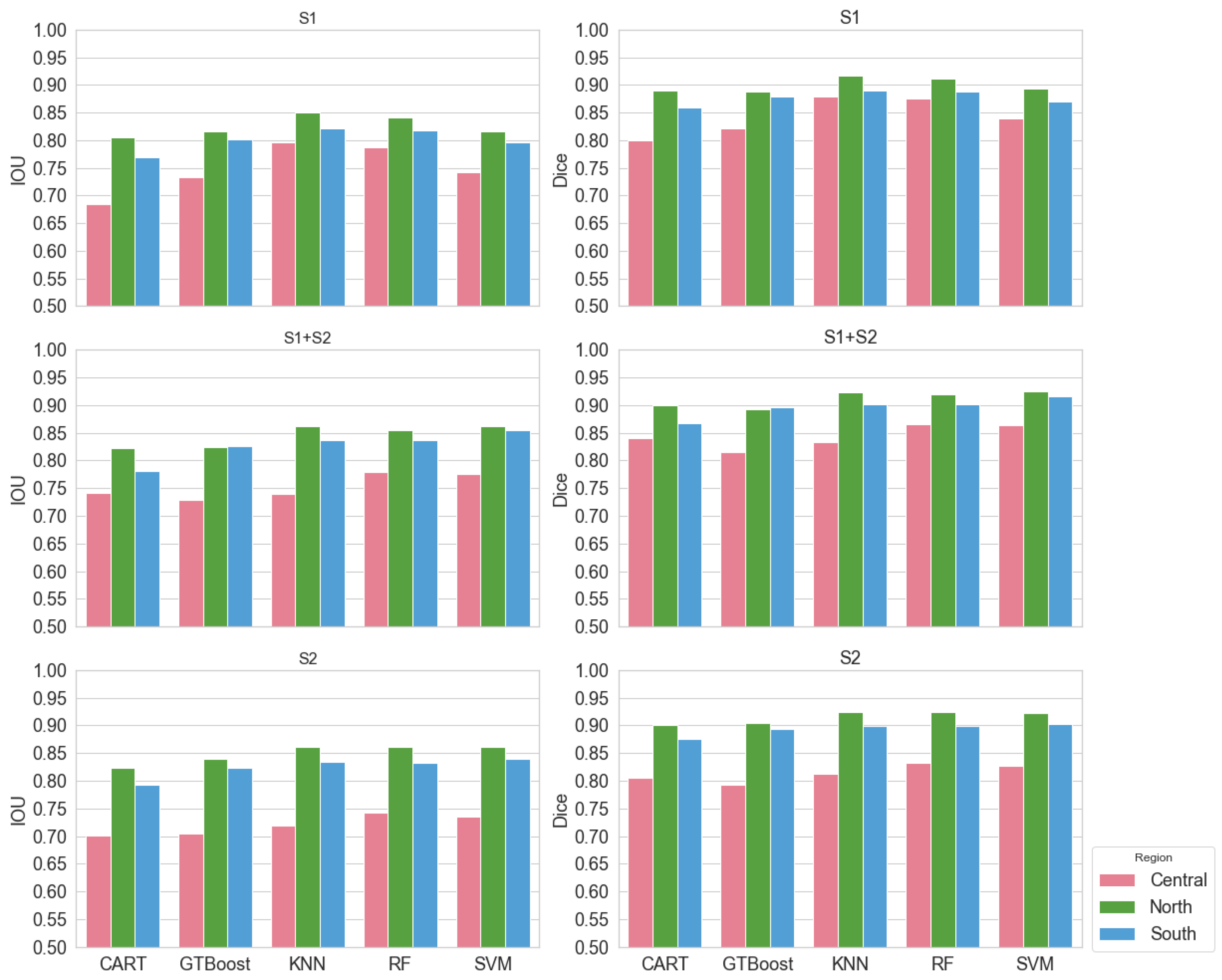
3.2. Classification Results

Following our proposed pipeline, the next step is the classification process. We present the results for the model training first (Section 3.2.1), and then we emphasize the different performances according to the rice field concentration in different patches (Section 3.2.2).

3.2.1. Overall Performance of the Models

When evaluating all the available patches according to Table 6, we can observe that, regarding the overall accuracy of the combinations between the datasets and models assessed, there was just a slight variation, with a maximum difference of 1% between CART S 1 and SVM S 1 + S 2 . This occurred because the proportion between irrigated rice and non-irrigated rice classes was very high (3.92) for some patches, with fewer than 10% of pixels representing irrigated rice fields.
We used the metrics IoU, Dice, omission error (OE), and commission error (CE) for a better assessment of the results. Hence, when evaluating these metrics considering all test patches, we found that the SVM S 1 + S 2 , KNN S 1 , and RF S 1 + S 2 combinations showed, in this order, the highest values of IoU (0.807, 0.803, and 0.801) and Dice (0.885, 0.882, and 0.881). On the other hand, the CART and GTBoost combinations for the three types of datasets and the SVM S 1 combination showed IoU values between 0.724 and 0.759 and Dice values between 0.829 and 0.851, representing the lowest values. Therefore, the maximum difference observed in the IoU and Dice values for the combinations tested was 8.3% and 5.6%, respectively.
When analyzing the omission and commission errors in Table 6 (considering all patches), we can see that, in general, the combinations tend to overestimate the irrigated rice class more than they omit it, with the commission error being much higher than the omission error. In general, the error of omission was below 10% for all combinations, except for CART S 2 (13.19%) and GTBoost S 2 (12.3%). We observed that, for all tested machine learning models, the use of only S2 images resulted in the highest omission errors, and the combined use of S1 and S2 data led, albeit slightly, to a reduction in omission errors for all the models.
However, the commission errors were all above 15% for all the models and datasets tested. The KNN and RF models showed the lowest commission errors regardless of the type of input dataset. Contrary to what occurred with the omission errors, when using only S2 images, all evaluated models presented lower commission error values, while using only S1 images resulted in higher commission errors for all the models.
Regardless of the model used, the central region of the study area proved to be the most challenging for irrigated rice field classification, yielding the lowest metric values, as shown in Figure 12. The southern and northern regions produced similar results, with the northern region showing higher classification quality. This outcome suggests that, despite the predominance of double-crop systems in the northern region and the predominance of the single-crop system in the southern region, the methodology and data used in this study did not encounter issues in classifying these areas. However, the models’ generalization only achieved moderate classification quality for the west-central region, considering the significantly different conditions in the area.
Topographically, radar/SAR systems face significant limitations due to interference and distortions caused by high elevation terrain. Despite all correction processes, such terrains remain challenging for radar imaging. Consequently, the west-central region of the Santa Catarina state, where rice is cultivated at altitudes above 700 m (available in Supplementary Materials Figure S9), exhibited the poorest classification results across all tested models, underscoring the difficulty of mapping rice fields in high altitude areas. A literature review along with our image analysis show that irrigated rice fields in high altitude regions, with less than 10% of irrigate rice fields, are typically small, fragmented, elongated areas located in valleys and slopes where water sources from rivers are accessible. Additionally, the incidence angle of Sentinel-1 (available in Supplementary Materials Figure S10) can cause variations in the VV, VH, CR, and RVIm time series values in these small areas.
Climatic factors also play a role in the classification results when using remote sensing, and they can be even more impactful when analyzing small fields. Rainfall affects SAR sensors, while scattered clouds impact optical imagery. In both cases, the small size of the fields (less than 1 hectare) means that even a medium-sized cloud or a high density of small clouds can significantly hinder field detection, as these fields are frequently not observed in the satellite images (available in Supplementary Materials Figure S11). The influence of climatic factors, particularly cloud cover, on the classification of small rice fields is extensively covered in the literature. As highlighted by Sakamoto et al. [68] and aligning with our observations, cloud cover significantly obstructs the detection of small rice fields, especially in areas where these fields are mixed with other land cover types. This contrasts with larger fields, where, even if one part is covered by clouds or cloud shadows on a given date, another part can be visible on a future date within the same month or within two months, allowing the creation of a good image mosaic.

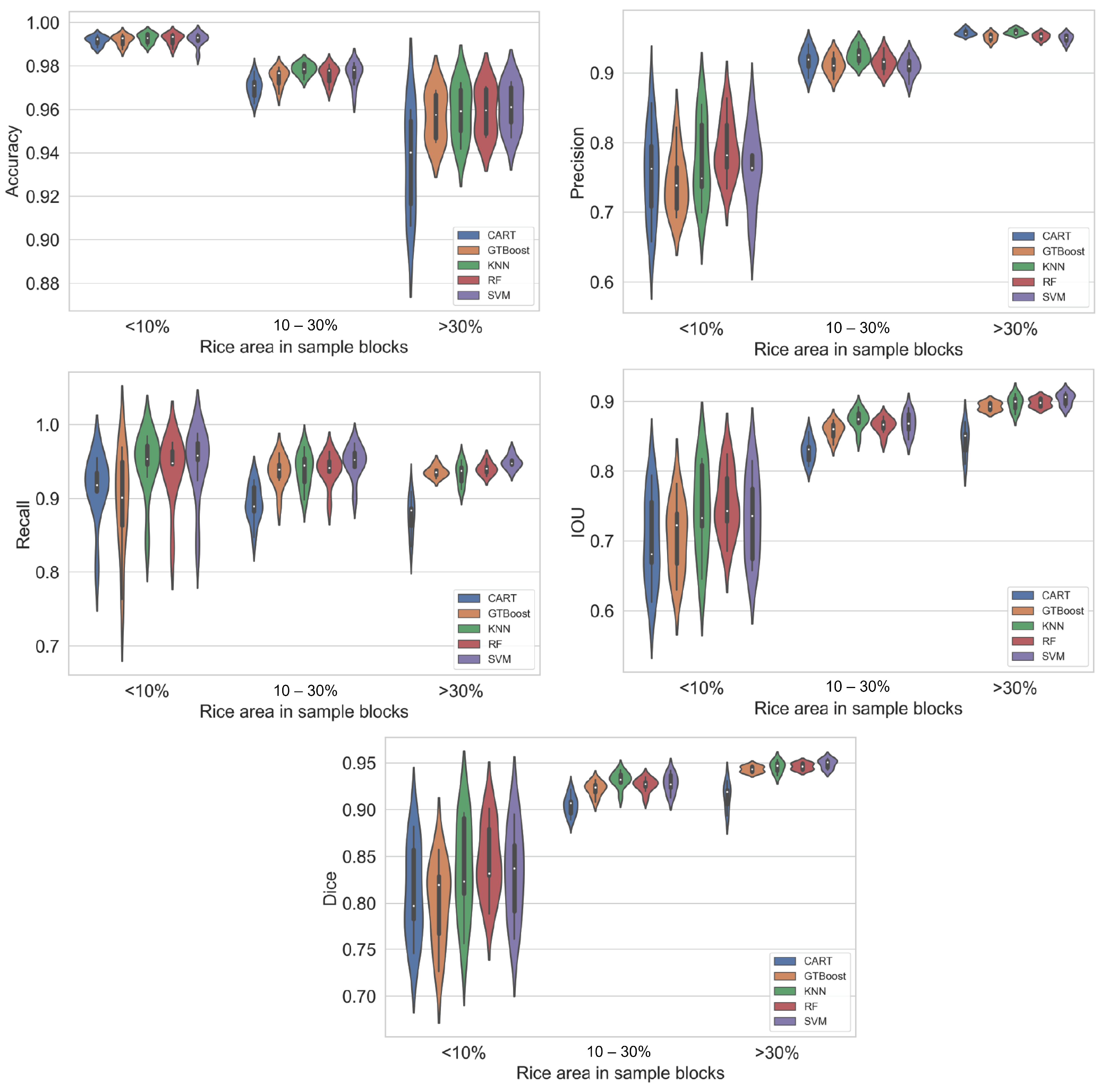
3.2.2. Performance of the Models Based on Rice Fileds Density

The SVM model, utilizing the merged S1+S2 dataset, had the highest performance in most metrics and scenarios, suggesting its capability to be used for irrigated rice field classification. Analysis of Figure 13 demonstrates that in test patches with a lower concentration of irrigated rice fields, less than 10%, the classification performance shows significant variability across models. IOU values ranged from 0.55 to 0.9 for CART, GTBoost, KNN, and SVM, and from 0.65 to 0.9 for RF. This variability can be attributed to the fragmentation of the 10% of rice into small or elongated fields, resulting in a lower classification quality with IOU values around 0.6. In contrast, when these irrigated rice areas, constituting up to 10%, are clustered in larger fields—either a single large field or up to two or three—the IOU values are generally closer to 0.9.
For regions where the rice area comprises 10–30% or more than 30% of the patches’ area, the variation is significantly reduced, with IOU values ranging from 0.85 to 0.9 (10–30%), and from 0.80 to 0.90 for CART and close to 0.9 for other models.
At the qualitative analysis level (Figure 14), differences between regions with varying rice planting densities are subtle and have a minimal impact on the classification of fields. However, areas with lower densities of irrigated rice fields tend to exhibit higher commission errors, as evidenced by a greater number of scattered misclassified points. Even after applying morphological opening and closing filters, these artifacts persisted, as a more aggressive filtering approach could compromise the delineation of irrigated rice fields.

4. Discussion

In this section, we present a discussion about our proposed pipeline performance. To perform this, we first discuss the time series clustering approach (Section 4.1). We focused on how our approach was able to automatically identify the different rice patterns in the Santa Catarina state and how that was useful in the pipeline process. Afterward, we shift our discussion to the classification approach (Section 4.2), contextualizing the discussion about the different models and rice density.

4.1. Irrigated Rice Time Series Clustering

The findings from the study highlight a significant contribution in the form of the detailed characterization of various types of irrigated rice cultivation across two cropping seasons. This was achieved using Sentinel-1 VV and VH polarizations, alongside CR and RVIm. Furthermore, the study integrates indices derived from Sentinel-2, such as the NDVI, EVI, NDWI, and MNDWI, offering a detailed evaluation of rice field dynamics.
Moreover, we utilized feature engineering methods involving soft-DTW and K-means algorithms to optimize and balance the input data, facilitating a more organized classification process in line with the method proposed by Guan et al. [22]. This method is based on temporal similarity clustering to categorize various rice cultivation types. Furthermore, exploratory data analysis was conducted to improve the model’s generalizability, ensuring it accurately reflects the diversity in rice growth patterns across different regions and farming techniques.
The NDVI proved to be the most robust index, effectively capturing multiple growth phases, including harvests and regrowth, while maintaining stability during peak vegetative stages. The ability to remain largely unsaturated during peak vegetative stages (between 160 and 200 Days of Season, DoS) underscores its applicability for tracking rice farming, corroborating the results of [69,70] regarding the use of the NDVI for mapping and monitoring rice fields. For rice cultivation, in particular, Rehman et al. [69] detected the saturation of the NDVI occurring between 0.76 and 0.78. Thus, in addition to being more effective in distinguishing regrowth cultivation, the NDVI does not exhibit significant saturation during the vegetative and peak vegetative growth phases—between DoS 160 and 200—in the context of the Santa Catarina state. The EVI also performs well in identifying regrowth cultivation; however, the distinctions between the initial and subsequent growth stages were more evident in the NDVI, underscoring its greater efficacy in representing the complete range of rice crop development. The NDWI, on the other hand, showed inverse patterns to the NDVI, indicating its utility in tracking water content during different stages of cultivation.
Our results indicate that VH polarization was more affected at the beginning of the crop season. Meanwhile, VV polarization was more consistent over time, due to the vertical structure of rice fields which minimizes the SAR penetration signal. This uniformity indicates that the VH curve can be useful to generalize single harvest irrigated rice field classification studies, corroborated by [13,71,72], who highlight VH as more useful than VV for mapping rice fields. This finding aligns with the observations by Phan et al. [73], who reported on VV’s fluctuation throughout the crop season and suggested combining it with VH for better classification results. The noted differentiation in clustering between the VV and VH polarizations is consistent with the findings of [55,74], who observed the different sensitivities of the SAR polarizations to different crop-type structures such as alfalfa, wheat, barley, corn, and soybeans and for different soil conditions, such as wet, dry, and tilled soil. RVIm was influenced by biomass and vegetation water content, reaching its peak during the rice grain filling and flowering stages, giving crucial insights into the crop’s developmental timeline [75]. Furthermore, the peak values in the RVIm and CR indices indicated increased volumetric scattering due to the formation of grain and leaf structures, while the lowest values aligned with maximum tiller development, occurring before the vegetative peak in the NDVI (Figure 6). This underscores the importance of these SAR indices in capturing early phenological signals.
In our results, we found out that the central region exhibits more heterogeneity, without a predominant pattern. According to Xu et al. [76], even minor shifts in the acquisition angle could lead to variations in backscattering, thus complicating the characterization of the area further.
An important limitation of the selection model that employs DTW in combination with K-means is the necessity for a pre-specified number of clusters (k) required by the K-means algorithm. In certain scenarios, especially with distinct behaviors or noisy time series, the clustering process may fail to accurately detect these patterns. Thus, the suggested methodology takes on a more generalized approach, emphasizing broad mapping over the detailed characterization of specific cultivation patterns.

4.2. Irrigated Rice Classification

One significant challenge in this research involved assessing the effectiveness of five distinct machine learning models in generalizing the classification of extensive irrigated rice areas (46,088 km2) by unifying various rice cultivation types into one irrigated rice category in Santa Catarina. The results demonstrated a robust methodology for extensive area classification, utilizing a range of spectral and temporal features. Moreover, we examined which machine learning model accessible on the Google Earth Engine (GEE) platform delivered the most precise classification of rice fields throughout various regions of Santa Catarina, providing insights for future extensive agricultural mapping.
Our results indicate a slight accuracy variation across the multiple stacks and models. These results can be due to a ratio between rice and background classes. In the study conducted by de Bem et al. [17], where the authors used only Sentinel-1 data in a deep learning model for rice mapping, they observed the same behavior. For the test sample patch, which had a 1:5 ratio between rice and background classes, the maximum accuracy difference observed by the authors did not exceed 3.92.
The rationale behind this phenomenon is explored and exemplified in the study published by Barsi et al. [77], where the authors demonstrated what happens with overall accuracy with a ratio of approximately 3/20 or 15% between the desired class (C) and the undesired class (NC). In this case, the authors showed that even though the user accuracy (precision) had a value below 70%, the producer accuracy (recall) presented a moderate value (82.1%), due to the high true negative rate (TNR) and high negative predictive value (NPV), at 95.3% and 97.7%, respectively, and the overall accuracy had a high value (93.8%). Thus, we highlight that due to the presence of test patches with fewer than 10% pixels representing irrigated rice, the overall accuracy is not sufficient to evaluate the model efficiency. Therefore, evaluating only the overall accuracy becomes insufficient to assess the combinations tested in this study.
The evaluation of machine learning classifiers for crop classification indicates that no individual algorithm consistently surpasses others in all scenarios. Research [20,78,79] has emphasized the advantages of SVM and RF classifiers in specific situations. The SVM has shown higher accuracy in several crop classification tasks, particularly with smaller datasets, outperforming other techniques such as Artificial Neural Networks (ANNs), CART, and maximum likelihood classifiers [80,81]. Nonetheless, the SVM’s accuracy is highly dependent on tuning parameters, while RF exhibits robustness and stability, maintaining high overall accuracy with minimal sensitivity to algorithm parameter adjustments [82]. Additionally, although the SVM often leads in accuracy, RF’s ensemble structure provides better resilience against the drawbacks of individual decision tree classifiers.
Recent studies highlight the effectiveness of integrating radar sensors, such as Sentinel-1, with optical sensors to boost crop classification accuracy, especially when utilizing RF and the SVM [83,84]. Although the SVM and GTBoost frequently achieve the highest accuracy in crop classification, RF remains a reliable option due to its robustness across various datasets and low sensitivity to parameter changes [79,85]. Our results are consistent with those of Trisasongko et al. [86] and Ahmed et al. [78], who found that the SVM surpassed RF and CART in crop discrimination tasks. Nonetheless, GBT and RF often produce similar outcomes, particularly when forecasting complex variables [79,87]. These observations indicate that despite the SVM frequently leading in accuracy, RF’s dependability and robustness position it as a strong candidate for crop classification.
When evaluating areas with varying percentages of rice plots alongside other land uses, several critical factors need to be considered. Typically, regions with lower rice cultivation percentages correspond to smallholder systems, which complicates accurate identification by any model. This challenge is exacerbated by diverse agricultural practices, regional topography, and climate, as well as sensor limitations.
From a crop management perspective, varied planting and harvesting schedules among farmers hinder the models’ ability to accurately capture these fields. Additionally, rice seed production farms, which follow different cultivation standards, add complexity to the classification process. In smallholder or family-owned farms, inter-cropping is common, leading to spectral mixing within pixels due to limited spatial resolution, which complicates rice field detection by models that do not account for this mixing.
Moreover, this challenge aligns with findings by Jin et al. [88], who noted that classifying small crop fields is difficult due to inherent heterogeneity, often resulting from mixed cropping practices. In regions with complex terrain, like Taiwan and Chongqing, where rice fields are small and irregularly shaped, spectral mixing often leads to significant classification uncertainties. This requires refined algorithms to accurately distinguish mixed pixels [89,90]. Effective remote sensing in these areas demands approaches that consider within-farm diversity and variations in cultivation practices.
To overcome the cloud cover limitation it was necessary a moderate cloud percentage threshold (50%) for image tiles in GEE. A higher threshold contaminates the average composition with clouds, while a lower threshold results in a collection with fewer images, making it impossible to create monthly compositions. A similar logic applies to radar data, where localized rainfall can introduce noise in the time series data of smaller fields. The necessity of setting a moderate cloud threshold, which we adopted using the GEE platform, is crucial for balancing image accessibility and quality. This method is similar to the one applied in the research by Wang et al. [90], where the frequent cloudy days in Chongqing created considerable challenges for optical remote sensing, hindering the capture of clear images during essential periods of rice growth.
Similarly to our observations for the central region of our study area, where rice is cultivated at altitudes above 700 m, Son et al. [89] reported that small and fragmented rice fields in Taiwan complicate the acquisition of high quality satellite imagery, leading to lower classification accuracies. Additionally, the topography in Taiwan exacerbates the mixed-pixel issues and boundary effects, which are also significant in our study when using radar.
Irrigated rice filed identification can be significantly affected by the 10-m spatial resolution of sensors used in this study, which may miss small fields due to spectral mixing. The incidence angle of Sentinel-1, illustrated in Supplementary Materials Figure S10, can also cause variations in VV, VH, CR, and RVIm time series values [76], as the regional diversity of samples often leads to generalized models.
The detection issues of small rice fields in complex terrains, as highlighted in this study, echo challenges noted by Son et al. [91]. Variations in backscatter due to incidence angles and mixed-pixel effects in small, dispersed rice fields contribute to mapping inaccuracies, especially in regions with significant elevation changes. This is evident in our study, where the poorest classification results were found in central high-altitude areas. Similarly, Wang et al. [90] emphasizes the need for specialized algorithms to address speckle noise and terrain factors in SAR data, enhancing the precision of rice field extraction in challenging environments.
In summary, the substantial influence of topographical variability, small field dimensions, and weather conditions on the precision of rice field classification via remote sensing methods has been reported in the literature. Our results add to this existing research by highlighting the necessity for customized strategies that tackle these unique issues, especially in areas with small, scattered, and high-altitude rice fields.
Another limitation of this classification method, as mentioned in Section 4.1 about the lack of specificity in time series extraction, is the generation of polygons devoid of detailed resolution at the smallholding or plot scale. This poses difficulties for temporal analysis because irrigated rice fields often utilize furrows and canals along plot boundaries and within the fields themselves. Consequently, fields classified as one unit may actually involve varying planting, harvesting, and management processes within the same area. This divergence can result in inaccuracies, especially when performing detailed analyses on small-scale farming operations.

5. Conclusions

Our proposed pipeline serves as an efficient way to perform temporal monitoring and classification of irrigated rice fields in large areas in Brazil. We observed that there are generally four main patterns of irrigated rice development in the Santa Catarina state, with the fact that in the northern and southern regions, there are two much more dominant cultivation patterns: double cropping in the north and single cropping in the south. In the central region, on the other hand, there is greater diversity in the types of irrigated rice cultivation.
Optical indices (EVI, NDVI, MNDWI) effectively tracked vegetative growth and water content, while radar data offered complementary insights into scattering mechanisms related to crop development. The NDVI is highlighted as the most efficient optical index to monitor the different vegetative stages. In terms of SAR data, VH polarization offered consistent clustering performance, particularly in single-cropping systems, and effectively differentiated cultivation types despite some noisiness. VV polarization demonstrated more variability, which limited its effectiveness for binary classification when used alone. The RVIm and CR indices provided valuable alternative clustering methods, with RVIm peaking during critical growth stages such as grain filling and flowering.
Machine learning classification models utilizing combined Sentinel-1 and Sentinel-2 datasets achieved the highest classification metrics with the SVM. The KNN and SVM models showed strong performance with the combined dataset, while GTBoost and RF models also performed effectively, with RF demonstrating robustness across datasets. Challenges such as spectral mixing in smaller fields and variations in topography and climate emphasized the need for multi-index approaches and diverse data sources to enhance the accuracy of rice field mapping in varied terrains.
Concerning the relevance of this study’s results for decision-making and planning in irrigated rice farming in Santa Catarina, we highlight the considerable importance of the suggested automated mapping methodology for both institutions and policymakers. Presently, most mapping in the region depends on semi-automated techniques. By implementing the proposed method, mapping becomes more efficient, allowing for near real-time annual evaluations. Furthermore, precise mapping of irrigated rice fields is essential in Santa Catarina due to the crop’s substantial water demands. Regular assessments of rice cultivation areas improve the monitoring of water resource utilization and distribution, aiding in more sustainable agricultural management.
As future work, we propose that this pipeline should be used with more optical data such as CBERS-4 and 4A, Amazonia, and Landsat-8, 9. Furthermore, we believe that NISAR and Biomass SAR should be tested in this pipeline in the future. Additionally, from a more technical perspective, future studies should explore models and approaches developed outside the GEE environment, such as scikit-learn and TensorFlow. This is important because some limitations arise from the parameter selection and processing constraints within the platform, and external tools could optimize data processing.

Supplementary Materials

The following supporting information can be downloaded at https://www.mdpi.com/article/10.3390/agriengineering7030065/s1. Figure S1: Spatial distribution of temporal patterns of the NDVI index for irrigated rice during the 2017/2018 (top map) and 2018/2019 (bottom map) plant growing seasons; Figure S2: Spatial distribution of temporal pattern of the Enhanced Vegetation Index (EVI) for irrigated rice, in the crops of 2017/2018 (top map) and 2018/2019 (bottom map) plant growing seasons; Figure S3: Spatial distribution of temporal patterns of the NDWI index for irrigated rice during the 2017/2018 (top map) and 2018/2019 (bottom map) plant growing seasons; Figure S4: Spatial distribution of temporal patterns of the MNDWI index for irrigated rice during the 2017/2018 (top map) and 2018/2019 (bottom map) plant growing seasons; Figure S5: Spatial distribution of temporal patterns of VH polarization for irrigated rice, in the 2017/2018 (top map) and 2018/2019 (bottom map) plant growing seasons; Figure S6: Spatial distribution of temporal patterns of VV polarization for irrigated rice, in the 2017/2018 (top map) and 2018/2019 (bottom map) plant growing seasons; Figure S7: Spatial distribution of temporal patterns of CR polarization for irrigated rice, in the 2017/2018 (top map) and 2018/2019 (bottom map) plant growing seasons; Figure S8: Spatial distribution of temporal patterns of RVIm polarization for irrigated rice, in the 2017/2018 (top map) and 2018/2019 (bottom map) plant growing seasons; Figure S9: Terrain elevation characterization of the state of Santa Catarina, derived from Shuttle Radar Topography Mission (SRTM) data at a 30 m spatial resolution; Figure S10: Incidence angle over the study area derived from the “angle” band of Sentinel-1B, using data from the COPERNICUS/S1_GRD image collection in Google Earth Engine; Figure S11: Representation of cloud and shadow cover in the undefined cluster group in south region on the clustering map of optical indices. Red contour indicates low quality images and green contour represents good quality images; Figure S12: Example of optical series discarded due to data absence for certain periods. This data was collected on South part of the study area, since the most problematic time-series were observed there; Figure S13: Example of linear interpolation and smoothing performed on the feasible time series data extracted from Sentinel-1 and Sentinel-2 satellites; Figure S14: General workflow to cluster irrigated rice time series and generate an irrigated rice binary map using different dataset combination and models.

Author Contributions

Conceptualization, A.D.B.G. and I.D.S.; methodology, A.D.B.G., I.D.S. and V.H.R.P.; software, A.D.B.G.; validation, A.D.B.G., I.D.S., V.H.R.P. and K.T.; formal analysis, A.D.B.G., I.D.S. and V.H.R.P.; investigation, A.D.B.G., I.D.S., V.H.R.P. and K.T.; resources, A.D.B.G., I.D.S., V.H.R.P. and K.T.; data curation, A.D.B.G., I.D.S. and V.H.R.P.; writing—original draft preparation, A.D.B.G.; writing—review and editing, A.D.B.G., I.D.S., V.H.R.P. and K.T.; visualization, A.D.B.G., I.D.S., V.H.R.P. and K.T.; supervision, I.D.S. and V.H.R.P.; project administration, I.D.S.; funding acquisition, I.D.S. All authors have read and agreed to the published version of the manuscript.

Funding

This study was financed in part by the Coordenação de Aperfeiçoamento de Pessoal de Nível Superior (CAPES), Brazil; Finance Code 001. The authors are grateful to the Brazilian National Council of Scientific and Technological Development (CNPq) for the Research Productivity Fellowship of Sanches, I.D [310042/2021-6].

Data Availability Statement

The data presented in this study are openly available in the “Characterization and Classification of Irrigated Rice in Santa Catarina” repository at https://doi.org/10.17632/3n8ms32thw.1 (reserved DOI). The original reference data are available from public websites: https://www.iff.sc.gov.br/dados-e-mapas (accessed on 8 March 2024, 2017/2018 season reference) and https://metadados.snirh.gov.br/geonetwork/srv/api/records/1ac9b37f-0745-44f9-a60b-6a2bd366bbe1 (accessed on 10 March 2024, 2018/2019 season reference).

Acknowledgments

The authors are grateful to the field agents from EPAGRI, especially Douglas George de Oliveira, for providing the rice field photos used in this research.

Conflicts of Interest

Author Kleber Trabaquini was employed by the company Santa Catarina Agricultural Research and Extension Corporation (EPAGRI). The remaining authors declare that the research was conducted in the absence of any commercial or financial relationships that could be construed as a potential conflict of interest.

References

  1. FAO-Food and Agriculture Organization of the United Nations. FAOSTAT: FAO Statistical Databases. 2022. Available online: https://www.fao.org/faostat/en/#data/QCL/visualize (accessed on 20 June 2023).
  2. CONAB-Companhia Nacional de Abastecimento. Acompanhamento da Safra Brasileira de Grãos-Safra 2023/24-6° Levantamento. 2024. Available online: https://www.conab.gov.br/info-agro/safras/graos/boletim-da-safra-de-graos/item/download/52225_79be7813e39c3746ab9121250bbfb5c5 (accessed on 15 August 2024).
  3. Chen, N.; Yu, L.; Zhang, X.; Shen, Y.; Zeng, L.; Hu, Q.; Niyogi, D. Mapping paddy rice fields by combining multi-temporal vegetation index and synthetic aperture radar remote sensing data using google earth engine machine learning platform. Remote Sens. 2020, 12, 2992. [Google Scholar] [CrossRef]
  4. Oad, V.K.; Dong, X.; Arfan, M.; Kumar, V.; Mohsin, M.S.; Saad, S.; Lü, H.; Azam, M.I.; Tayyab, M. Identification of shift in sowing and harvesting dates of rice crop (L. Oryza sativa) through remote sensing techniques: A case study of larkana district. Sustainability 2020, 12, 3586. [Google Scholar] [CrossRef]
  5. Zhang, J.; Wu, H.; Zhang, Z.; Zhang, L.; Luo, Y.; Han, J.; Tao, F. Asian Rice Calendar Dynamics Detected by Remote Sensing and Their Climate Drivers. Remote Sens. 2022, 14, 4189. [Google Scholar] [CrossRef]
  6. do Vale, M.L.C.; Hickel, E.R.; de Andrade, A.; Back, A.J.; Pandolfo, C.; de Oliveira, D.G.; Wickert, E.; Masiero, F.C.; Martins, G.N.; Guimarães, G.G.F.; et al. Recomendações para a produção de arroz irrigado em Santa Catarina: 4a. ed. Sist. Produção 2022, 4, 1587. [Google Scholar]
  7. Ramadhani, F.; Pullanagari, R.; Kereszturi, G.; Procter, J. Automatic mapping of rice growth stages using the integration of sentinel-2, mod13q1, and sentinel-1. Remote Sens. 2020, 12, 3613. [Google Scholar] [CrossRef]
  8. Stroppiana, D.; Boschetti, M.; Azar, R.; Barbieri, M.; Collivignarelli, F.; Gatti, L.; Fontanelli, G.; Busetto, L.; Holecz, F. In-season early mapping of rice area and flooding dynamics from optical and SAR satellite data. Eur. J. Remote Sens. 2019, 52, 206–220. [Google Scholar] [CrossRef]
  9. Prudente, V.H.R.; Martins, V.S.; Vieira, D.C.; e Silva, N.R.d.F.; Adami, M.; Sanches, I.D. Limitations of cloud cover for optical remote sensing of agricultural areas across South America. Remote Sens. Appl. Soc. Environ. 2020, 20, 100414. [Google Scholar] [CrossRef]
  10. Whitcraft, A.K.; Vermote, E.F.; Becker-Reshef, I.; Justice, C.O. Cloud Cover throughout the Agricultural Growing Season: Impacts on Passive Optical Earth Observations. Remote Sens. Environ. 2015, 156, 438–447. [Google Scholar] [CrossRef]
  11. Veloso, A.; Mermoz, S.; Bouvet, A.; Le Toan, T.; Planells, M.; Dejoux, J.F.; Ceschia, E. Understanding the temporal behavior of crops using Sentinel-1 and Sentinel-2-like data for agricultural applications. Remote Sens. Environ. 2017, 199, 415–426. [Google Scholar] [CrossRef]
  12. Dingle Robertson, L.; Davidson, A.; McNairn, H.; Hosseini, M.; Mitchell, S.; De Abelleyra, D.; Verón, S.; Cosh, M.H. Synthetic Aperture Radar (SAR) image processing for operational space-based agriculture mapping. Int. J. Remote Sens. 2020, 41, 7112–7144. [Google Scholar] [CrossRef]
  13. Bazzi, H.; Baghdadi, N.; El Hajj, M.; Zribi, M.; Minh, D.H.T.; Ndikumana, E.; Courault, D.; Belhouchette, H. Mapping paddy rice using Sentinel-1 SAR time series in Camargue, France. Remote Sens. 2019, 11, 887. [Google Scholar] [CrossRef]
  14. Phan, H.; Le Toan, T.; Bouvet, A.; Nguyen, L.D.; Pham Duy, T.; Zribi, M. Mapping of rice varieties and sowing date using X-band SAR data. Sensors 2018, 18, 316. [Google Scholar] [CrossRef] [PubMed]
  15. Yonezawa, C.; Watanabe, M. Airborne L-band SAR observation for paddy rice fields in semi-mountainous region. In Proceedings of the 2017 IEEE International Geoscience and Remote Sensing Symposium (IGARSS), Fort Worth, TX, USA, 23–28 July 2017; pp. 5073–5076. [Google Scholar] [CrossRef]
  16. Crisóstomo de Castro Filho, H.; Abílio de Carvalho Júnior, O.; Ferreira de Carvalho, O.L.; Pozzobon de Bem, P.; dos Santos de Moura, R.; Olino de Albuquerque, A.; Rosa Silva, C.; Guimaraes Ferreira, P.H.; Fontes Guimarães, R.; Trancoso Gomes, R.A. Rice crop detection using LSTM, Bi-LSTM, and machine learning models from Sentinel-1 time series. Remote Sens. 2020, 12, 2655. [Google Scholar] [CrossRef]
  17. de Bem, P.P.; de Carvalho Júnior, O.A.; de Carvalho, O.L.F.; Gomes, R.A.T.; Guimarães, R.F.; Pimentel, C.M.M. Irrigated rice crop identification in Southern Brazil using convolutional neural networks and Sentinel-1 time series. Remote Sens. Appl. Soc. Environ. 2021, 24, 100627. [Google Scholar] [CrossRef]
  18. Fernandes Filho, A.S.; Fonseca, L.M.G.; Bendini, H.d.N. Mapping Irrigated Rice in Brazil Using Sentinel-2 Spectral–Temporal Metrics and Random Forest Algorithm. Remote Sens. 2024, 16, 2900. [Google Scholar] [CrossRef]
  19. Zhao, R.; Li, Y.; Ma, M. Mapping paddy rice with satellite remote sensing: A review. Sustainability 2021, 13, 503. [Google Scholar] [CrossRef]
  20. Sujud, L.; Jaafar, H.; Hassan, M.A.H.; Zurayk, R. Cannabis detection from optical and RADAR data fusion: A comparative analysis of the SMILE machine learning algorithms in Google Earth Engine. Remote Sens. Appl. Soc. Environ. 2021, 24, 100639. [Google Scholar] [CrossRef]
  21. Onojeghuo, A.O.; Blackburn, G.A.; Wang, Q.; Atkinson, P.M.; Kindred, D.; Miao, Y. Mapping paddy rice fields by applying machine learning algorithms to multi-temporal Sentinel-1A and Landsat data. Int. J. Remote Sens. 2018, 39, 1042–1067. [Google Scholar] [CrossRef]
  22. Guan, X.; Huang, C.; Liu, G.; Meng, X.; Liu, Q. Mapping rice cropping systems in Vietnam using an NDVI-based time-series similarity measurement based on DTW distance. Remote Sens. 2016, 8, 19. [Google Scholar] [CrossRef]
  23. Kontgis, C.; Schneider, A.; Ozdogan, M. Mapping rice paddy extent and intensification in the Vietnamese Mekong River Delta with dense time stacks of Landsat data. Remote Sens. Environ. 2015, 169, 255–269. [Google Scholar] [CrossRef]
  24. Lei, T.C.; Wan, S.; Wu, Y.C.; Wang, H.P.; Hsieh, C.W. Multi-temporal data fusion in MS and SAR images using the dynamic time warping method for paddy Rice classification. Agriculture 2022, 12, 77. [Google Scholar] [CrossRef]
  25. IBGE-Brazilian Institute of Geography and Statistics. Panorama-Santa Catarina. 2021. Available online: https://cidades.ibge.gov.br/brasil/sc/panorama (accessed on 8 July 2024).
  26. Monteiro, M.A. Caracterização climática do estado de Santa Catarina: Uma abordagem dos principais sistemas atmosféricos que atuam durante o ano. Geosul 2001, 16, 69–78. Available online: https://periodicos.ufsc.br/index.php/geosul/article/view/14052 (accessed on 10 July 2024).
  27. CONAB-Companhia Nacional de Abastecimento. Acompanhamento da Safra Brasileira de Grãos-Safra 2022/23. 2023. Available online: https://www.conab.gov.br/info-agro/safras/graos/boletim-da-safra-de-graos/item/download/47720_642c6cc3d60e063c21c87a3094e7f5f7 (accessed on 26 May 2024).
  28. EPAGRI-Empresa de Pesquisa Agropecuária e Extensão Rural de Santa Catarina. Zoneamento Agroecológico e Socioeconômico. 2022. Available online: https://ciram.epagri.sc.gov.br/index.php/solucoes/zoneamento/ (accessed on 30 March 2024).
  29. Fritzsons, E.; Mantovani, L.E.; Wrege, M.S. Relaçãoo entre altitude e temperatura: Uma contribuição ao zoneamento climático no estado de Santa Catarina, Brasil. Rev. Bras. De Climatol. 2016, 18. [Google Scholar] [CrossRef]
  30. Wrege, M.S.; Steinmetz, S.; Reisser Junior, C.; de Almeida, I.R. Atlas climático da Região Sul do Brasil: Estados do Paraná, Santa Catarina e Rio Grande do Sul; Embrapa Clima Temperado: Pelotas, Brazil; Embrapa Florestas: Colombo, Sri Lanka, 2012; Available online: http://www.infoteca.cnptia.embrapa.br/infoteca/handle/doc/1045852 (accessed on 28 March 2024).
  31. Vibrans, A.C.; Nicoletti, A.L.; Liesenberg, V.; Refosco, J.C.; de Araújo Kohler, L.P.; Bizon, A.R.; Lingner, D.V.; Dal Bosco, F.; Bueno, M.M.; da Silva, M.S.; et al. MonitoraSC: Um novo mapa de cobertura florestal e uso da terra de Santa Catarina. Agropecuária Catarin. 2021, 34, 42–48. [Google Scholar] [CrossRef]
  32. Garcia, A.D.B.; Islam, M.S.; Prudente, V.H.R.; Sanches, I.D.; Cheng, I. Irrigated rice-field mapping in Brazil using phenological stage information and optical and microwave remote sensing. Appl. Comput. Geosci. 2025, 25, 100223. [Google Scholar] [CrossRef]
  33. Garcia, A.D.B.; Prudente, V.H.R.; da Silva, D.T.; Chaves, M.E.D.; Trabaquini, K.; Sanches, I.D. Detailed Mapping of Irrigated Rice Fields Using Remote Sensing data and Segmentation Techniques: A case of study in Turvo, Santa Catarina, Brazil. J. Inf. Data Manag. 2025, 16, 92–109. [Google Scholar] [CrossRef]
  34. Torres, R.; Snoeij, P.; Geudtner, D.; Bibby, D.; Davidson, M.; Attema, E.; Potin, P.; Rommen, B.; Floury, N.; Brown, M.; et al. GMES Sentinel-1 mission. Remote Sens. Environ. 2012, 120, 9–24. [Google Scholar] [CrossRef]
  35. Dasari, K.; Anjaneyulu, L. Importance of Speckle filter window Size and its impact on Speckle reduction in SAR images. Int. J. Adv. Microw. Technol. (IJAMT) 2017, 2, 98–102. [Google Scholar]
  36. Garcia, A.D.B.; Sanches, I.D.; Adami, M.; Gama, F.F. Performance evaluation of speckle filters for paddy rice areas based on Sentinel-1 satellite images. In Proceedings of the Anais do XX Simpósio Brasileiro de Sensoriamento Remoto, Florianópolis, Brazil, 2–5 April 2023; Volume 20, pp. 644–647. Available online: https://proceedings.science/sbsr-2023/trabalhos/perfomance-evaluation-of-speckle-filters-for-paddy-rice-areas-based-on-sentinel?lang=en (accessed on 10 October 2024).
  37. Quegan, S.; Yu, J.J. Filtering of multichannel SAR images. IEEE Trans. Geosci. Remote Sens. 2001, 39, 2373–2379. [Google Scholar] [CrossRef]
  38. Mullissa, A.; Vollrath, A.; Odongo-Braun, C.; Slagter, B.; Balling, J.; Gou, Y.; Gorelick, N.; Reiche, J. Sentinel-1 sar backscatter analysis ready data preparation in Google Earth Engine. Remote Sens. 2021, 13, 1954. [Google Scholar] [CrossRef]
  39. Doblas, J.; Frery, A.C.; Sant’Anna, S.J.S.; Carneiro, A.; Shimabukuro, Y.E. Assessment of nonlocal means stochastic distances speckle reduction for SAR time series. In Proceedings of the 2021 IEEE International Geoscience and Remote Sensing Symposium IGARSS, Brussels, Belgium, 11–16 July 2021; pp. 3265–3268. [Google Scholar] [CrossRef]
  40. Santos, E.P.d.; Moreira, M.C.; Fernandes-Filho, E.I.; Demattê, J.A.M.; Dionizio, E.A.; Silva, D.D.d.; Cruz, R.R.P.; Moura-Bueno, J.M.; Santos, U.J.d.; Costa, M.H. Sentinel-1 imagery used for estimation of soil organic carbon by dual-polarization SAR vegetation indices. Remote Sens. 2023, 15, 5464. [Google Scholar] [CrossRef]
  41. Mandal, D.; Kumar, V.; Ratha, D.; Dey, S.; Bhattacharya, A.; Lopez-Sanchez, J.M.; McNairn, H.; Rao, Y.S. Dual polarimetric radar vegetation index for crop growth monitoring using sentinel-1 SAR data. Remote Sens. Environ. 2020, 247, 111954. [Google Scholar] [CrossRef]
  42. Copernicus. New Products Available: The Sensor Invariant Atmospheric Correction (SIAC) Based Mosaics Albedo. 2023. Available online: https://land.copernicus.eu/en/news/new-products-available-the-sensor-invariant-atmospheric-correction-siac-based-mosaics-albedo (accessed on 23 July 2024).
  43. Yin, F.; Lewis, P.E.; Gómez-Dans, J.L. Bayesian atmospheric correction over land: Sentinel-2/MSI and Landsat 8/OLI. Geosci. Model Dev. 2022, 15, 7933–7976. [Google Scholar] [CrossRef]
  44. Google. Google Earth Engine Developers: Resampling and Reducing Resolution. 2024. Available online: https://developers.google.com/earth-engine/guides/resample (accessed on 1 May 2024).
  45. Jiang, Z.; Huete, A.R.; Didan, K.; Miura, T. Development of a two-band enhanced vegetation index without a blue band. Remote Sens. Environ. 2008, 112, 3833–3845. [Google Scholar] [CrossRef]
  46. Fraga, H.; Amraoui, M.; Malheiro, A.C.; Moutinho-Pereira, J.; Eiras-Dias, J.; Silvestre, J.; Santos, J.A. Examining the relationship between the Enhanced Vegetation Index and grapevine phenology. Eur. J. Remote Sens. 2014, 47, 753–771. [Google Scholar] [CrossRef]
  47. Halos, S.H.; Abed, F.G. Effect of spring vegetation indices NDVI & EVI on dust storms occurrence in Iraq. In AIP Conference Proceedings; AIP Publishing: Karbala City, Iraq, 2019; Volume 2144, p. 040015. [Google Scholar] [CrossRef]
  48. Sanches, I.D.; Feitosa, R.Q.; Diaz, P.M.A.; Soares, M.S.; Luiz, A.J.L.; Schultz, B.; Maurano, L.E.P. Campo Verde Database: Seeking to Improve Agricultural Remote Sensing of Tropical Areas. IEEE Geosci. Remote Sens. Lett. 2018, 15, 369–373. [Google Scholar] [CrossRef]
  49. Sanches, I.D.; Feitosa, R.Q.; Montibeller, B.; Achanccaray Diaz, P.M.; Luiz, A.J.B.; Soares, M.D.; Prudente, V.H.R.; Vieira, D.C.; Maurano, L.E.P.; Happ, P.N.; et al. First Results of the Lem Benchmark Database for Agricultural Applications. Int. Arch. Photogramm. Remote. Sens. Spat. Inf. Sci. 2020, XLIII-B5-2020, 251–256. [Google Scholar] [CrossRef]
  50. Oldoni, L.V.; Sanches, I.D.; Picoli, M.C.A.; Covre, R.M.; Fronza, J.G. LEM+ dataset: For agricultural remote sensing applications. Data Brief 2020, 33, 106553. [Google Scholar] [CrossRef]
  51. ANA-Agência Nacional de Águas e Saneamento. Mapeamento do Arroz Irrigado no Brasil. 2020. Available online: https://metadados.snirh.gov.br/geonetwork/srv/api/records/1ac9b37f-0745-44f9-a60b-6a2bd366bbe1 (accessed on 7 August 2023).
  52. Reyes, F.; Casa, R.; Tolomio, M.; Dalponte, M.; Mzid, N. Soil properties zoning of agricultural fields based on a climate-driven spatial clustering of remote sensing time series data. Eur. J. Agron. 2023, 150, 126930. [Google Scholar] [CrossRef]
  53. Beuchle, R.; Grecchi, R.C.; Shimabukuro, Y.E.; Seliger, R.; Eva, H.D.; Sano, E.; Achard, F. Land cover changes in the Brazilian Cerrado and Caatinga biomes from 1990 to 2010 based on a systematic remote sensing sampling approach. Appl. Geogr. 2015, 58, 116–127. [Google Scholar] [CrossRef]
  54. Li, H.; Song, X.P.; Hansen, M.C.; Becker-Reshef, I.; Adusei, B.; Pickering, J.; Wang, L.; Wang, L.; Lin, Z.; Zalles, V.; et al. Development of a 10-m resolution maize and soybean map over China: Matching satellite-based crop classification with sample-based area estimation. Remote Sens. Environ. 2023, 294, 113623. [Google Scholar] [CrossRef]
  55. McNairn, H.; Champagne, C.; Shang, J.; Holmstrom, D.; Reichert, G. Integration of optical and Synthetic Aperture Radar (SAR) imagery for delivering operational annual crop inventories. ISPRS J. Photogramm. Remote Sens. 2009, 64, 434–449. [Google Scholar] [CrossRef]
  56. Tavenard, R.; Faouzi, J.; Vandewiele, G.; Divo, F.; Androz, G.; Holtz, C.; Payne, M.; Yurchak, R.; RuBwurm, M.; Kolar, K.; et al. Tslearn, a machine learning toolkit for time series data. J. Mach. Learn. Res. 2020, 21, 1–6. [Google Scholar]
  57. Cuturi, M. Fast global alignment kernels. In Proceedings of the 28th International Conference on Machine Learning (ICML-11), Bellevue, WA, USA, 28 June–2 July 2011; pp. 929–936. Available online: http://www.icml-2011.org/papers/489_icmlpaper.pdf (accessed on 11 July 2024).
  58. Cuturi, M.; Blondel, M. Soft-dtw: A differentiable loss function for time-series. In Proceedings of the International Conference on Machine Learning. PMLR, Sydney, Australia, 6–11 August 2017; pp. 894–903. Available online: http://proceedings.mlr.press/v70/cuturi17a/cuturi17a.pdf (accessed on 5 July 2024).
  59. Jiang, J.; Lai, S.; Jin, L.; Zhu, Y. Dsdtw: Local representation learning with deep soft-dtw for dynamic signature verification. IEEE Trans. Inf. Forensics Secur. 2022, 17, 2198–2212. [Google Scholar] [CrossRef]
  60. Maxwell, A.E.; Warner, T.A.; Fang, F. Implementation of machine-learning classification in remote sensing: An applied review. Int. J. Remote Sens. 2018, 39, 2784–2817. [Google Scholar] [CrossRef]
  61. Talukdar, S.; Singha, P.; Mahato, S.; Pal, S.; Liou, Y.A.; Rahman, A. Land-use land-cover classification by machine learning classifiers for satellite observations—A review. Remote Sens. 2020, 12, 1135. [Google Scholar] [CrossRef]
  62. Pech-May, F.; Aquino-Santos, R.; Rios-Toledo, G.; Posadas-Durán, J.P.F. Mapping of land cover with optical images, supervised algorithms, and google earth engine. Sensors 2022, 22, 4729. [Google Scholar] [CrossRef]
  63. Salas, E.A.L.; Kumaran, S.S.; Bennett, R.; Willis, L.P.; Mitchell, K. Machine Learning-Based Classification of Small-Sized Wetlands Using Sentinel-2 Images. AIMS Geosci. 2024, 10, 62–79. [Google Scholar] [CrossRef]
  64. Friedman, J.H. Stochastic gradient boosting. Comput. Stat. Data Anal. 2002, 38, 367–378. [Google Scholar] [CrossRef]
  65. Liu, L.; Guo, Y.; Li, Y.; Zhang, Q.; Li, Z.; Chen, E.; Yang, L.; Mu, X. Comparison of machine learning methods applied on multi-source medium-resolution satellite images for Chinese pine (Pinus tabulaeformis) extraction on Google Earth Engine. Forests 2022, 13, 677. [Google Scholar] [CrossRef]
  66. Liu, Z.; Li, N.; Wang, L.; Zhu, J.; Qin, F. A multi-angle comprehensive solution based on deep learning to extract cultivated land information from high-resolution remote sensing images. Ecol. Indic. 2022, 141, 108961. [Google Scholar] [CrossRef]
  67. Yuan, K.; Zhuang, X.; Schaefer, G.; Feng, J.; Guan, L.; Fang, H. Deep-learning-based multispectral satellite image segmentation for water body detection. IEEE J. Sel. Top. Appl. Earth Obs. Remote Sens. 2021, 14, 7422–7434. [Google Scholar] [CrossRef]
  68. Sakamoto, T.; Sprague, D.S.; Okamoto, K.; Ishitsuka, N. Semi-automatic classification method for mapping the rice-planted areas of Japan using multi-temporal Landsat images. Remote Sens. Appl. Soc. Environ. 2018, 10, 7–17. [Google Scholar] [CrossRef]
  69. Rehman, T.H.; Borja Reis, A.F.; Akbar, N.; Linquist, B.A. Use of normalized difference vegetation index to assess N status and predict grain yield in rice. Agron. J. 2019, 111, 2889–2898. [Google Scholar] [CrossRef]
  70. Gu, Y.; Wylie, B.K.; Howard, D.M.; Phuyal, K.P.; Ji, L. NDVI saturation adjustment: A new approach for improving cropland performance estimates in the Greater Platte River Basin, USA. Ecol. Indic. 2013, 30, 1–6. [Google Scholar] [CrossRef]
  71. Chang, L.; Chen, Y.T.; Wang, J.H.; Chang, Y.L. Rice-field mapping with Sentinel-1A SAR time-series data. Remote Sens. 2020, 13, 103. [Google Scholar] [CrossRef]
  72. Fatchurrachman; Rudiyanto; Soh, N.C.; Shah, R.M.; Giap, S.G.E.; Setiawan, B.I.; Minasny, B. Automated near-real-time mapping and monitoring of rice growth extent and stages in Selangor Malaysia. Remote Sens. Appl. Soc. Environ. 2023, 31, 100993. [Google Scholar] [CrossRef]
  73. Phan, H.; Le Toan, T.; Bouvet, A. Understanding dense time series of Sentinel-1 backscatter from rice fields: Case study in a province of the Mekong Delta, Vietnam. Remote Sens. 2021, 13, 921. [Google Scholar] [CrossRef]
  74. McNairn, H.; Brisco, B. The application of C-band polarimetric SAR for agriculture: A review. Can. J. Remote Sens. 2004, 30, 525–542. [Google Scholar] [CrossRef]
  75. Nasirzadehdizaji, R.; Balik Sanli, F.; Abdikan, S.; Cakir, Z.; Sekertekin, A.; Ustuner, M. Sensitivity analysis of multi-temporal Sentinel-1 SAR parameters to crop height and canopy coverage. Appl. Sci. 2019, 9, 655. [Google Scholar] [CrossRef]
  76. Xu, S.; Qi, Z.; Li, X.; Yeh, A.G.O. Investigation of the effect of the incidence angle on land cover classification using fully polarimetric SAR images. Int. J. Remote Sens. 2019, 40, 1576–1593. [Google Scholar] [CrossRef]
  77. Barsi, A.; Kugler, Z.; László, I.; Szabó, G.; Abdulmutalib, H.M. Accuracy dimensions in remote sensing. Int. Arch. Photogramm. Remote Sens. Spat. Inf. Sci. 2018, 42, 61–67. [Google Scholar] [CrossRef]
  78. Ahmed, S.; Mahmoud, A.S.; Farg, E.; Mohamed, A.M.; Moustafa, M.S.; Abutaleb, K.; Saleh, A.M.; AbdelRahman, M.A.; AbdelSalam, H.M.; Arafat, S.M. Investigation on the use of ensemble learning and big data in crop identification. Heliyon 2023, 9, e13339. [Google Scholar] [CrossRef]
  79. Gupta, P.; Kanga, S.; Mishra, V.N.; Kumar, S.; Singh, T.S. A Comparative Study and Machine Learning Enabled Efficient Classification for Multispectral Data in Agriculture. Baghdad Sci. J. 2024, 21, 2462. [Google Scholar] [CrossRef]
  80. Nitze, I.; Schulthess, U.; Asche, H. Comparison of machine learning algorithms random forest, artificial neural network and support vector machine to maximum likelihood for supervised crop type classification. In Proceedings of the 4th International Conference on Geographic Object-Based Image Analysis—GEOBIA, Rio de Janeiro, Brazil, 7–9 May 2012; Volume 79, p. 3540. Available online: http://mtc-m16c.sid.inpe.br/col/sid.inpe.br/mtc-m18/2012/05.30.22.11/doc/index.html (accessed on 1 August 2024).
  81. Qian, Y.; Zhou, W.; Yan, J.; Li, W.; Han, L. Comparing machine learning classifiers for object-based land cover classification using very high resolution imagery. Remote Sens. 2014, 7, 153–168. [Google Scholar] [CrossRef]
  82. Fang, P.; Zhang, X.; Wei, P.; Wang, Y.; Zhang, H.; Liu, F.; Zhao, J. The classification performance and mechanism of machine learning algorithms in winter wheat mapping using Sentinel-2 10 m resolution imagery. Appl. Sci. 2020, 10, 5075. [Google Scholar] [CrossRef]
  83. Denize, J.; Hubert-Moy, L.; Betbeder, J.; Corgne, S.; Baudry, J.; Pottier, E. Evaluation of using sentinel-1 and-2 time-series to identify winter land use in agricultural landscapes. Remote Sens. 2018, 11, 37. [Google Scholar] [CrossRef]
  84. Orynbaikyzy, A.; Gessner, U.; Mack, B.; Conrad, C. Crop type classification using fusion of sentinel-1 and sentinel-2 data: Assessing the impact of feature selection, optical data availability, and parcel sizes on the accuracies. Remote Sens. 2020, 12, 2779. [Google Scholar] [CrossRef]
  85. Dimov, D.; Löw, F.; Ibrakhimov, M.; Stulina, G.; Conrad, C. SAR and optical time series for crop classification. In Proceedings of the 2017 IEEE International Geoscience and Remote Sensing Symposium (IGARSS), Fort Worth, TX, USA, 23–28 July 2017; pp. 811–814. [Google Scholar] [CrossRef]
  86. Trisasongko, B.H.; Panuju, D.R.; Paull, D.J.; Jia, X.; Griffin, A.L. Comparing six pixel-wise classifiers for tropical rural land cover mapping using four forms of fully polarimetric SAR data. Int. J. Remote Sens. 2017, 38, 3274–3293. [Google Scholar] [CrossRef]
  87. Freeman, E.A.; Moisen, G.G.; Coulston, J.W.; Wilson, B.T. Random forests and stochastic gradient boosting for predicting tree canopy cover: Comparing tuning processes and model performance. Can. J. For. Res. 2016, 46, 323–339. [Google Scholar] [CrossRef]
  88. Jin, Z.; Azzari, G.; You, C.; Di Tommaso, S.; Aston, S.; Burke, M.; Lobell, D.B. Smallholder maize area and yield mapping at national scales with Google Earth Engine. Remote Sens. Environ. 2019, 228, 115–128. [Google Scholar] [CrossRef]
  89. Son, N.T.; Chen, C.F.; Chen, C.R.; Toscano, P.; Cheng, Y.S.; Guo, H.Y.; Syu, C.H. A phenological object-based approach for rice crop classification using time-series Sentinel-1 Synthetic Aperture Radar (SAR) data in Taiwan. Int. J. Remote Sens. 2021, 42, 2722–2739. [Google Scholar] [CrossRef]
  90. Wang, L.; Ma, H.; Li, J.; Gao, Y.; Fan, L.; Yang, Z.; Yang, Y.; Wang, C. An automated extraction of small-and middle-sized rice fields under complex terrain based on SAR time series: A case study of Chongqing. Comput. Electron. Agric. 2022, 200, 107232. [Google Scholar] [CrossRef]
  91. Son, N.T.; Chen, C.F.; Chen, C.R.; Minh, V.Q. Assessment of Sentinel-1A data for rice crop classification using random forests and support vector machines. Geocarto Int. 2018, 33, 587–601. [Google Scholar] [CrossRef]
Figure 1. Map showing the study area’s location in the eastern part of the Santa Catarina state, Brazil, divided into N—north, C—central, and S—south regions. Inside these regions there are the train (green) and test (yellow) patches, based on the reference rice fields (red).
Agriengineering 07 00065 g001
Figure 2. Distribution and statistical summary of irrigated rice field sizes by region: number of fields, mean, median, maximum, and minimum sizes (ha).
Agriengineering 07 00065 g002
Figure 3. Flowchart detailing the processes for extracting the most prevalent time series and mapping the distribution of different crop types across regions. The last two green boxes represent outputs used to support decision-making in the classification process.
Agriengineering 07 00065 g003
Figure 4. Flowchart illustrating the process of generating binary images to differentiate between irrigated rice and non-irrigated areas. The first green box (top-left) is derived from the decisions made based on the outcomes of Figure 3. The last three green boxes (bottom-right) are categorized according to the density of irrigated rice areas per sample patch.
Agriengineering 07 00065 g004
Figure 5. Spatial distribution of temporal patterns of the NDVI index for irrigated rice fields in the study area (N—north, C1 and C2—central, S—south regions). Clusters 0, 1, 2, and 3 are different types of irrigated rice time series. The undefined class corresponds to areas that were not possible to cluster into groups.
Agriengineering 07 00065 g005
Figure 6. Spatial distribution of temporal patterns of the NDWI index for irrigated rice fields in the study area (N—north, C1 and C2—central, S—south regions). Clusters 0, 1, 2, and 3 are different types of irrigated rice time series. The undefined class corresponds to areas that were not possible to cluster into groups.
Agriengineering 07 00065 g006
Figure 7. Spatial distribution of temporal pattern clusters of the Vertical emitter–Vertical receiver (VV) index for irrigated rice fields in the study area (N—north, C1 and C2—central, S—south regions). Clusters 0, 1, 2, and 3 are different types of irrigated rice time series. The undefined class corresponds to areas that were not possible to cluster into groups.
Agriengineering 07 00065 g007
Figure 8. Spatial distribution of temporal pattern clusters of the Cross-Ratio (CR) index for irrigated rice fields in the study area (N—north, C1 and C2—central, S—south regions). Clusters 0, 1, 2, and 3 are different types of irrigated rice time series. The undefined class corresponds to areas that were not possible to cluster into groups.
Agriengineering 07 00065 g008
Figure 9. Most representative growth pattern of irrigated rice by region for optical indices, considering the more frequent clusterings in both seasons (2017/2018 and 2018/2019).
Agriengineering 07 00065 g009
Figure 10. Most representative growth pattern of irrigated rice by region for SAR polarization and indices, considering the more frequent clusterings in both seasons (2017/2018 and 2018/2019).
Agriengineering 07 00065 g010
Figure 11. Growth behavior of irrigated rice according to different indices, sensors, and stages of the growth cycle. (A) Time series pattern for NDVI and NDWI for single-harvest rice fields. (B) Time series pattern for VH and VV polarizations for single-harvest rice fields. (C) Time series pattern for NDVI and NDWI for double-harvest rice fields. (D) Time series pattern for VH and VV polarizations for double-harvest rice fields. At the bottom, the photos illustrate the condition of the irrigated rice fields at various stages of crop development. Source of photos: Douglas George de Oliveira and EPAGRI.
Agriengineering 07 00065 g011
Figure 12. Overall comparison of instance segmentation evaluation metrics for different models, regions, and datasets.
Agriengineering 07 00065 g012
Figure 13. Performance metrics for rice field classifications considering the testing patches with less then 10% of rice, between 10 and 30%, and over 30%.
Agriengineering 07 00065 g013
Figure 14. Qualitative analysis for different rice field classification models, considering the testing patches with less then 10% of rice, between 10 and 30%, and over 30% for different image datasets. The initial three columns are images from the west-central region, characterized by higher elevation. Columns 4, 5, and 6 are images from the north region, notable for its higher occurrence of double-harvest. The final three columns are images from the south region, where single-harvest is prevalent and rice fields are typically more extensive. In the figure, black represents ‘non-rice fields’, while yellow areas represent ‘rice fields’.
Agriengineering 07 00065 g014
Table 1. Seasonal timeline of irrigated rice phenological stages by regions in eastern part of Santa Catarina, Brazil.
RegionAugSepOctNovDecJanFebMarApr
NorthS/ES/E/VDS/E/VDS/E/VDVD/FGF/MM/HH 
CentralS/ES/E/VDS/E/VDS/E/VDVD/FF/GFGF/M/HM/HH
SouthS/ES/E/VDS/E/VDS/E/VDVD/FF/GFGF/M/HM/HH
Sowing (S), Emergence (E), Vegetative Development (VD), Flowering (F), Grain Filling (GF), Maturation (M), and Harvest (H). Adapted from [27].
Table 2. Characteristics of Sentinel-1 imagery utilized in every phase of this study.
CharacteristicValue
PlatformB
Image formatGRD (Ground Range Detected)
Acquisition modeIW (Interferometric Wide Swath)
Acquisition orbitDescending
Incidence angle29° to 46°
Resolution10 m
Swath width250 Km
PolarizationVV and VH
Frequency5.4 (GHz)
Revisit time12 days
Dataset availabilityApr/2016 to Dec/2021
Sentinel-1B ceased operations on 23 December 2021 due to a power supply anomaly.
Table 3. Characteristics of Sentinel-2/MSI (platforms A and B) spectral bands utilized in every phase of this study.
Spectral Bands (µm)Resolution (m)Band ID
Blue (0.45–0.52)10B2
Green (0.54–0.57)10B3
Red (0.65–0.68)10B4
NIR (0.78–0.89)10B8
SWIR 1 (1.56–1.65)20B11
NIR = Near Infrared, SWIR = Shortwave Infrared.
Table 4. Statistical summary of the data patches and fields by region, including total and train–test split analysis.
RegionTrainTestTotalMean f · p 1 Median f · p 1 Max. f · p 1 Min. f · p 1
North22103246301723
Central882611429181701
South38276589415202
Total14863211
Note: f · p 1 : fields per patch.
Table 5. Machine learning models and their parameter configurations used in this study.
ModelParameters
CARTmaxNodes: default (null)
minLeafPopulation: default (1)
GTBoostnumberOfTrees: 50
shrinkage: default (0.005)
samplingRate: default (0.7)
maxNodes: default (null)
loss: default (LeastAbsoluteDeviation)
seed: 1
KNNk: 5
searchMethod: AUTO
metric: default (EUCLIDEAN)
RFnumberOfTrees: 50
variablesPerSplit: default (sqrt of number of variables)
minLeafPopulation: default (1)
bagFraction: default (0.5)
maxNodes: default (null)
seed: 1
SVMdecisionProcedure: default (Voting)
svmType: C_SVC
kernelType: RBF
shrinking: default (true)
gamma: 0.30
cost: 50
seed: 1
Table 6. Performance of each classification model for binary irrigated rice fields and non-irrigated rice with different dataset combinations for all test patches. Bold numbers indicate the top five highest-performing results for each metric across the evaluated datasets.
ModelAccuracyPrecisionRecallIOUDiceOECE
C A R T S 1 0.9770.7890.9040.7240.8299.60%21.07%
C A R T S 2 0.9790.8470.8680.7510.84413.19%15.28%
C A R T S 1 + S 2 0.9800.8060.9260.7550.8517.37%19.41%
G T B o o s t S 1 0.9820.7940.9070.7520.8389.32%20.64%
G T B o o s t S 2 0.9840.8180.8770.7580.83712.33%18.17%
G T B o o s t S 1 + S 2 0.9840.7920.9150.7590.8418.45%20.81%
K N N S 1 0.9840.8490.9420.8030.8825.78%15.05%
K N N S 2 0.9850.8270.9180.7760.8588.23%17.26%
K N N S 1 + S 2 0.9860.8110.9560.7830.8654.39%18.86%
R F S 1 0.9830.8330.9460.7940.8775.39%16.73%
R F S 2 0.9850.8500.9110.7890.8688.93%15.03%
R F S 1 + S 2 0.9850.8370.9490.8010.8815.14%16.26%
S V M S 1 0.9810.7810.9530.7510.8444.71%21.89%
S V M S 2 0.9850.8390.9200.7860.8667.97%16.13%
S V M S 1 + S 2 0.9870.8330.9590.8070.8854.05%16.68%
Disclaimer/Publisher’s Note: The statements, opinions and data contained in all publications are solely those of the individual author(s) and contributor(s) and not of MDPI and/or the editor(s). MDPI and/or the editor(s) disclaim responsibility for any injury to people or property resulting from any ideas, methods, instructions or products referred to in the content.

