Abstract
Energy expenditure constitutes a significant portion of total operational costs in greenhouse crop production. Developing accurate energy consumption prediction models presents crucial theoretical foundations for optimizing the environmental control strategies aimed at energy efficiency enhancement. This study focuses on steel-frame solar greenhouses without back slopes in Xinjiang’s Tianshan North Slope region. A physical model was established using thermodynamic equilibrium analysis, elucidating the energy exchange mechanisms between internal and external environments. Key parameters, including outdoor temperature and solar radiation, were identified as primary input variables through systematic energy flow characterization. Building upon this theoretical framework, we developed an enhanced prediction model (WOA-ELM) by integrating the Whale Optimization Algorithm (WOA) with an Extreme Learning Machine (ELM). The WOA’s global optimization capabilities were employed to refine the connection weights between input-hidden layers and optimize hidden neuron thresholds. Comparative evaluations against conventional artificial neural networks (ANNs), radial basis function neural networks (RBFNN), and baseline ELM models were conducted under diverse meteorological conditions. Experimental results demonstrate the superior performance of WOA-ELM across multiple metrics. Under overcast conditions, the model achieved a root mean square error (RMSE) of 0.423, coefficient of determination (R2) of 0.93, and mean absolute error (MAE) of 0.252. In clear weather scenarios, performance further improved with RMSE = 0.27, R2 = 0.96, and MAE = 0.063. The comprehensive evaluation ranked model effectiveness as WOA-ELM > ELM > BP > RBF. These findings substantiate that the hybrid WOA-ELM architecture, combining physical mechanism interpretation with intelligent parameter optimization, delivers enhanced prediction accuracy across varying weather patterns. This research provides valuable insights for energy load management in backslope-less steel-frame greenhouses, offering theoretical guidance for thermal environment regulation and sustainable operation.
1. Introduction
Greenhouses represent a type of high-energy-consumption agricultural production facility, with operational energy consumption accounting for 30–40% of the total production costs, making it a primary constraint on greenhouse productivity [1]. This issue is particularly pronounced in northern China, where overwintering production requires substantial heating energy, leading to high production costs that have become a major challenge for greenhouse operations during the winter months [2,3]. In Xinjiang, facility agriculture primarily relies on solar greenhouses. Under the influence of the “dual carbon” policy, solar greenhouses in the northern slopes of the Tianshan Mountains have transitioned from traditional energy-based heating methods to electric hot air heating systems. However, the higher cost of electric heating compared to traditional energy sources has forced many solar greenhouses to cease production during winter, as the energy consumption for heating exceeds the economic viability in this region [4]. Consequently, the significant energy demand for winter heating has emerged as a critical factor limiting greenhouse production in this area [5]. To enhance energy utilization efficiency and reduce operational costs, the establishment of a greenhouse energy consumption prediction model is essential. Such a model can predict and analyze greenhouse energy consumption, providing a theoretical foundation for greenhouse selection, design, and control strategies.
Extensive research has been conducted both domestically and internationally on greenhouse energy consumption prediction methods, which can be broadly categorized into two approaches: mechanism modeling and black box modeling. Jolliet et al. [6] developed a dynamic model to predict the energy consumption of a glass greenhouse based on the heat balance equation. Their experimental results demonstrate that the error between simulated and measured annual energy consumption values was less than 10%. Singh et al. [7] derived a greenhouse energy consumption model by integrating energy balance equations for various components of the greenhouse, reporting a mean percentage error of 18.42% in total energy consumption prediction. Ahamed et al. [8] estimated hourly heating demand based on the heat balance of greenhouse air, achieving an average percentage error of 8.7% and an average relative root mean square error of 11.5% for hourly heating prediction. Their model proved to be a valuable tool for greenhouse designers and researchers in designing energy-efficient greenhouses across different locations. Dai et al. [9] analyzed greenhouse energy consumption using a microclimate model, incorporating the effects of canopy transpiration to establish a predictive energy consumption model. Xu et al. [10] focused on a glass-type greenhouse, analyzing radiation, convection, heat, and mass exchange caused by crop transpiration to develop a temperature and humidity model. Y. Shen [11] established a mathematical model of energy consumption for a Venlo-type greenhouse based on the principle of energy conservation. By employing three optimization algorithms to determine uncertain parameters and integrating weather forecast data, the model successfully predicted greenhouse energy consumption under varying weather conditions. Wang [12] developed a basic energy consumption prediction model for modern greenhouses in southern regions based on microclimate simulation analysis, enabling the calculation of greenhouse energy consumption. Dai Jianfeng et al. [13] established a computerized prediction system for the base energy consumption required for winter heating of greenhouses, providing a foundation for further research on optimal greenhouse environment regulation in China. Yao Yiping et al. [14] integrated greenhouse crop growth models and energy consumption prediction models to assess the investment risks of different greenhouse types in China. Their work included greenhouse climate zoning and the integration of energy consumption and crop potential yield estimation systems, offering valuable insights for optimizing greenhouse environment regulation from an energy consumption perspective. While mechanism modeling [15] provides in-depth understanding and explanation, it is often limited by the complexity and difficulty of determining the parameters. Additionally, it cannot overcome constraints related to time, geography, and greenhouse type, as some physical parameters vary with changes in these factors, limiting its universal applicability.
With the rapid advancement of artificial intelligence algorithms and their widespread application in agricultural facilities, the development of greenhouse energy consumption prediction models has gradually shifted from mechanistic models to black box models [16,17]. The accuracy of black box models relies on the dataset and algorithm structure. Although the training process can be time-consuming, these models offer fast prediction speeds post-training and provide a simpler approach to predicting greenhouse energy consumption. Morteza et al. [18] employed a multilayer inverse neural network to predict temperature and energy losses in a semi-solar greenhouse in Azerbaijan, Iran. The simulation results were compared with experimental values, confirming the model’s accuracy. Trejo-Perea et al. [19] utilized a multilayer feed-forward neural network to model greenhouse energy consumption, achieving a prediction accuracy of 95%. De Zwart [20] applied the greenhouse climate and control model KASPRO to simulate greenhouse microclimates while predicting energy consumption, enabling the simulation of energy-saving strategies in greenhouse production. Khoshnevisan B [21] established a greenhouse energy consumption prediction model based on artificial neural networks (ANNs), achieving a coefficient of determination of 0.998, indicating excellent agreement between the model’s predictions and actual data. Özden S [22] developed an ANN-based greenhouse energy consumption prediction model, incorporating input variables such as internal temperature, external temperature, and soil temperature, which effectively predicted greenhouse energy consumption. Chen et al. [23] used a self-accelerating genetic particle swarm algorithm to identify difficult-to-determine parameters in the physical model of a greenhouse, establishing an energy consumption prediction model for semi-enclosed greenhouses. This model was used to predict daily energy consumption under varying outdoor temperatures and solar radiation levels, providing guidance for greenhouse energy design and management. Zhang Yunhe et al. [24] addressed the issue of excessive energy consumption and waste in northern glass greenhouses by establishing an energy consumption prediction model based on LSTM neural networks. This model accurately predicted energy consumption, offering a theoretical basis for precise energy control. Zhang Yuchen et al. [25] employed partial least squares regression to predict heat release from the walls of solar greenhouses, determining heating demand by combining wall heat release and greenhouse heat load. Currently, neural networks, as mature data mining tools, can solve complex and nonlinear mapping problems. However, they are prone to falling into local optima and suffer from slow convergence speeds. In recent years, bionic intelligent algorithms, such as particle swarm optimization and artificial fish swarm algorithms, have developed rapidly. Among these, the Whale Optimization Algorithm (WOA) stands out for its simplicity, fewer parameters, and superior performance in finding optimal solutions compared to other algorithms. While WOA has been widely used for adjusting and optimizing building energy models, its application in greenhouse environment modeling remains limited.
Currently, most international research focuses on glass intelligent greenhouses, while the structural design of daylight greenhouses is unique to China. Consequently, foreign research findings on greenhouse energy consumption prediction models can only serve as a reference for studies on daylight greenhouses in China, providing a theoretical foundation. In this study, an Extreme Learning Machine (ELM) neural network is employed to construct an energy consumption prediction model for daylight greenhouses. To enhance the model’s prediction accuracy and address the challenges in determining the connection weight matrix between the input layer and hidden layer, as well as the threshold values of neurons in the hidden layer of the ELM model, this paper proposes the use of the Whale Optimization Algorithm (WOA) to optimize the parameters of the ELM model. The WOA-ELM-based energy consumption prediction model for solar greenhouses offers a theoretical basis for optimizing energy-saving control strategies and reducing energy consumption.
2. Materials and Methods
2.1. Experimental Greenhouse
The test site was Sanping Teaching Practice Base of Xinjiang Agricultural University, with latitude and longitude of 43.92° N, 87.35° E. The solar greenhouse for the test was located in the north–south direction, with an east–west length of 44 m, a span of 8 m, a spine height of 2.6 m, a back wall height of 1.9 m, a front wall height of 0.6 m, and no back slopes. The front roof of the greenhouse is made of PO plastic film, which is covered with a heat preservation quilt. The greenhouse has skylights (5 in total) in the east–west direction, with heaters (15 kW power) and roll-up control equipment, of which the heaters are located in the center of the greenhouse. The switching of the heaters, the opening of the heat preservation blanket and the opening angle of the skylight are controlled by the computer, and the structure of the greenhouse is shown in Figure 1. During the test period, tomatoes were planted in the greenhouse in a north–south direction with row spacing of 30 cm and plant spacing of 37 cm.
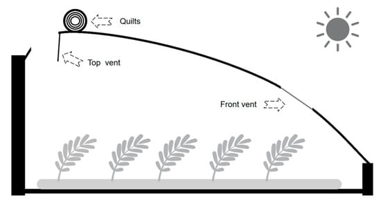
Figure 1.
Greenhouse diagram.
2.2. Experimental Method
The test period was from December 2023 to January 2024 and from December 2024 to January 2024, which is the lowest time of the oligo-sunshine temperature in the northern slope of Tianshan Mountain in Xinjiang, and the crop needs to be heated for safe overwintering. Since crops have different temperature requirements at different growth stages, tomato was in the fruiting stage during the test period, and the appropriate growth temperatures are shown in Table 1. Combined with the analysis of outdoor meteorological conditions, cloudy conditions will continue to dissipate heat after uncovering the curtain, so the choice of heating equipment during the day after uncovering the curtain set value most open for 11 °C, closed for 15 °C, the night set value open for 9 °C, closed for 13 °C. When the indoor temperature is higher than 30 °C, the skylight is opened for ventilation, and the average ventilation time is 20 min. The historical status of the operation of the indoor environmental control equipment (skylight, heat preservation quilt, heat fan, etc.) is collected in real time and automatically stored by the self-developed IoT monitoring platform, and the collected content includes the name of the equipment, the type of equipment operation (opening, closing, uncovering, shutting down the curtains), and the time of operation, etc. The greenhouse has a total of six environmental factors (opening, closing, uncovering, shutting down). A total of six environmental factors are collected in the greenhouse (Figure 2), and the collected environmental parameters include: indoor air temperature, indoor air humidity, indoor back wall temperature, indoor total solar radiation, outdoor total solar radiation, and outdoor air temperature. The indoor and outdoor environmental data were collected every 10 min, and the power consumption data of the greenhouse operation were recorded and uploaded to the database every 10 min.

Table 1.
Test-instrument-related parameters.
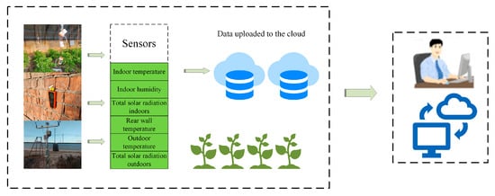
Figure 2.
Data collection process. Add arrows to indicate a progressive relationship.
Distribution of Test Instruments and Measurement Points
A total of 10 environmental factors, 3 crop growth parameters and power consumption in the greenhouse were collected by sensors. The environmental parameters collected included: indoor air temperature, indoor air humidity, indoor soil temperature, inner surface temperature of the mulch layer, temperature of the back wall, total indoor solar radiation, total outdoor solar radiation, outdoor air humidity, outdoor air temperature and outdoor wind speed. Crop growth parameter information collection includes leaf temperature, crop leaf area index, and crop extinction coefficient. The distribution points of greenhouse environmental monitoring are shown in Figure 3, and the accuracy of indoor and outdoor related monitoring instruments are shown in Table 2.
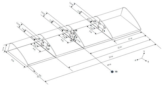
Figure 3.
Greenhouse measurement points diagram.
Table 2.
Test-instrument-related parameters.
2.3. Energy Consumption Prediction Model Construction Method
In this work, the heat exchange equations for each physical process in the greenhouse (e.g., heat transfer from enclosure, heat exchange from ventilation, crop transpiration, etc.) are established according to the principle of heat balance, and the mathematical expressions of the mechanism model are constructed so as to clarify the input variables (e.g., outdoor temperature, solar radiation, etc.) and output variables (energy consumption of greenhouse) of the system identification model. By analyzing the measured meteorological data and energy consumption data inside and outside the greenhouse, the structural reasonableness of the mechanism model is verified, and the key uncertain parameters in the model (e.g., integrated heat transfer coefficient, equipment efficiency, etc.) are identified. The dynamic relationships in the mechanistic model that are difficult to describe accurately are transformed into black-box modules to be identified, and a “grey-box” modeling framework is formed—i.e., the main structure of the model is determined by the mechanistic equations, and the uncertain parameters are optimized by the systematic identification method, so as to obtain the predictive model of greenhouse energy consumption that is both physically interpretable and data-driven accurate. This process reflects the guiding role of the mechanistic model for system identification: the physical modeling clarifies the input-output relationships and constrains the parameter ranges, provides a priori knowledge for data-driven parameter identification, and avoids the irrational structure or overfitting problems that may occur in the pure black-box model.
3. Construction of the Prediction Model
3.1. Model Building
The energy exchange between the greenhouse and the outside world involves a variety of factors, including the heating system, ventilation, plants, etc., inside the greenhouse and the air and solar radiation outside the greenhouse. Based on the principle of conservation of energy, the rate of change in air temperature inside the greenhouse is expressed as the result of heat exchange between the substances inside and outside the greenhouse. The energy required by the greenhouse heating system can be obtained from the temperature differential equation conversion, which can be expressed as
where reflects the rate of change in temperature in the greenhouse with time; reflects indoor air density, kg/m3; reflects the heat per unit volume of moist air, J/(kg∙k); reflects the energy input required to maintain the set temperature in the greenhouse, W; , , , reflects the convective heat transfer energy of indoor air with crops, back walls, soil, and interior coverings; Reflects solar radiant energy, W; reflects indoor temperature and outside heat transfer energy, W; reflects the energy gained from heating, W; reflects energy lost from indoor ventilation, W; reflects energy absorbed by crop transpiration, W.
According to the theorems of heat conduction energy exchange, mass and heat transfer energy exchange and crop latent and sensible heat exchange and the characteristics of the test greenhouse, the greenhouse energy consumption equation is
where , , , , reflect the area of crop canopy, back wall surface, soil surface, mulch (inner mulch), and mulch light transmission, m2, respectively; , , , reflect the convective heat transfer coefficients of the crop leaf to air, the back wall surface to air, the soil surface to air, and the inner mulch layer to air, respectively, W/m2∙K; , , , , , reflect the temperatures of indoor air, crop leaves, back wall surfaces, inner mulch surfaces, and outdoor air, respectively, K; reflects as greenhouse solar transmittance, derived by extrapolation of solar radiation values measured indoors and outdoors; reflects as the total solar radiation outside the greenhouse, W/m2; reflects the heat transfer coefficient of the covering material, W/m2∙K; reflecting the thermal effect of the heating system (supplied by the manufacturer); reflects the power of the heating system, W; reflects the slope of the saturated water vapor pressure versus temperature curve, kPa/°C; reflects soil heat flux, MJ/(m−2∙d); reflects the hygrometer constant, kPa/°C; , reflect the saturated and actual water vapor pressure of the air inside the greenhouse, kPa, respectively; reflects the density of net radiative heat flow obtained from the crop canopy, MJ/(m−2∙d); reflects the number of sunroof openings; reflects the length of the skylight, m; reflects the skylight width, m; reflects the acceleration of gravity, m/s2; reflects the angle between the skylight and the horizontal plane (the skylight in the greenhouse is parallel to the horizontal plane, take 180°), rad; reflects the sunroof opening angle, rad.
Where the convective heat transfer coefficients of the indoor air to the crop, back wall, and soil are simplified as [26], and the crop, back wall, and soil temperatures are simplified as
The convective heat transfer coefficient between the indoor air and the inner surface of the inner covering [26]:
convective heat transfer coefficient between the covering material and the outdoor air [26]:
where reflects the outdoor wind speed, m/s, which is obtained from the literature [27]:
The difference between the saturated and actual water vapor pressure of the air inside a greenhouse can be expressed as a function of temperature and relative humidity:
where reflects the indoor relative humidity, %; reflects the net shot above the canopy, W/m2; , reflect the crop extinction coefficient and leaf area index, both of which are measured by the plant canopy analyzer.
Equations (3)–(8) were substituted into Equation (1), and Matlab software R2016a was used to establish a physical model for predicting greenhouse energy consumption.
3.2. Sensitivity Analysis
Sensitivity analysis is the study and prediction of the extent to which changes in these attributes affect the model output values, assuming that the model is represented as ( is the attribute value of the model) such that each attribute varies within its range of values. Sensitivity analysis is a method that quantitatively describes the degree of importance of input variables to output variables, and is used to study the relationship between input and output variables and to identify important factors that affect simulation results. In this paper, sensitivity analysis is performed using the Genizi method, which decomposes the regressed sample coefficient of determination into a component that corresponds to the independent variable, which is non-negative. For the variable, the Genizi method is defined as
where reflects the number of independent variables; reflects the square root of a positive definite symmetric matrix; represents the critical (marginal) correlation between the independent and dependent variables, and the correlation coefficient is obtained by calculating the ratio of the covariance to the standard deviation. There are many parameters in the greenhouse energy consumption model, and many of them are affected by climate, materials, environment, measurement conditions and other factors, making it difficult to obtain their actual values directly. If these unknown parameters are identified directly, the amount of calculation is too large, and it is difficult to ensure the accuracy of the calculation results. The sensitivity test of parameters can determine the degree of influence of parameter changes on the model, and determine the uncertain parameters that need to be optimized and identified. The parameters in the physical model were analyzed according to the measured environmental parameters inside and outside the greenhouse and the energy consumption values, which were reduced to the determined and uncertain parameters in the model, of which the constant parameters in the model are shown in Table 3 below.
Table 3.
Test-instrument-related parameters.
Sensitivity analysis of uncertainties affecting greenhouse energy consumption was carried out and the results are shown in Figure 4 below. By analyzing the sensitivity, indoor temperature was the most sensitive variable, followed by total outdoor solar radiation, outdoor temperature, total indoor solar radiation, indoor humidity, back wall temperature, mulch temperature, crop canopy temperature, outdoor humidity, soil temperature, wind speed, and wind direction, respectively. The sensitivity analysis of the Genizi method showed that outdoor temperature, total outdoor solar radiation, total indoor solar radiation, indoor humidity, indoor temperature, and back wall temperature had the highest degree of influence on greenhouse energy consumption. Of these, indoor temperature is the most sensitive variable and directly determines the heating demand of the greenhouse; total outdoor solar radiation and temperature significantly contribute to energy consumption by affecting the heat exchange outside the greenhouse; total indoor solar radiation is involved in the internal heat gain, and humidity regulation is closely related to greenhouse energy consumption. Variations in these parameters make the largest contribution to model output, and prioritizing them ensures that the model captures the key drivers.
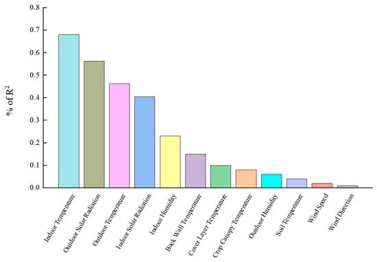
Figure 4.
Sensitivity analysis of energy consumption parameters.
4. Construction of the Prediction Model
4.1. Extreme Learning Machine
Extreme Learning Machine (ELM) is a learning method for single hidden layer feedforward neural networks, the structure usually includes input, hidden and output layers [28,29]. ELM solves the problem of slow speed of traditional machine learning by randomly generating the weights and biases of the nodes in the hidden layer, and combining with linear regression to calculate the output weights.
Assuming a series of sample data (), where , , the output of the ELM model for a neural network with input layer neurons, hidden layer neurons and a single output layer neuron is
where is the connection weight between the input layer neuron and the hidden layer neuron, ; is the threshold of the hidden layer; is the connection weight between the hidden layer neuron and the output layer neuron.
Among them, the activation function is a nonlinear segmented continuous function that satisfies the generalized approximation ability theorem of ELM, and the commonly used activation functions are Sigmoid function, sine function, hardlim function and so on. The sigmoid function outputs values mapped to the interval [0, 1], which highly matches the range of normalized environmental input parameters and energy consumption output data. This allows for the direct establishment of a nonlinear relationship between inputs and outputs, reducing error propagation during data conversion. Moreover, its smooth nonlinear characteristics better fit the mixed “gradual change—abrupt change” features of energy consumption data. Therefore, the sigmoid function is selected in this paper, with the corresponding functional expression being
The goal of single hidden layer neural network learning is to minimize the error in the output, denoted as
That is, there exist , and such that the sample output value is
4.2. Principles of Whale Optimization Algorithm
Whale Optimization Algorithm (WOA) is an optimization algorithm based on group intelligence, which was proposed by Australian scholars Mirjalili and Lewis in 2016, and is often combined with other algorithms to find the optimal operation of the model [30,31,32]. WOA employs a dual-strategy optimization approach of “encircling prey—spiral bubble net hunting.” In the initial phase, it performs global search to cover potential optimal solutions for ELM weights and thresholds, adapting to complex features where energy consumption and environmental factors are coupled. In the later phase, it conducts localized fine-grained optimization to capture the nonlinear “gradual change—abrupt change” patterns in energy consumption. Furthermore, WOA features fewer parameters, lower tuning complexity, and high tolerance for outdoor meteorological data noise. It adapts well to the low-sunlight and temperature-fluctuation scenarios of greenhouses in the northern slopes of the Tianshan Mountains in Xinjiang, ensuring training efficiency. This aligns strongly with the requirements for constructing gray-box models based on “mechanism + data-driven” approaches. Key whale behaviors include encircling prey, capturing prey, and searching for prey [33,34].
- (1)
- Surrounding the prey
A humpback whale’s ability to form an enclosure by constantly approaching its prey while hunting can be simplified into the following mathematical model:
where reflects the distance between the position of an individual in the humpback whale population and the global optimum position of the humpback whale population; is reflected as the current number of iterations; is reflected as the location of the current optimal solution; reflects the number of the next iteration; is reflected as a convergence factor.
- (2)
- Spiral bubble mesh hunting
Humpback whales catch their prey by creating bubble nets, mathematically modeled as follows:
where denotes the distance between the whale and the prey, the current optimal solution; reflects the constant coefficient that determines the shape of the individual whale’s helix as it spirals forward, with taking the value of 1 being a normal logarithmic helix; reflects a random number, taking values between [−1, 1].
- (3)
- Random search
Humpback whales search for prey in the vast ocean, and in the initial phase, when > 1, the whales update their search position based on randomly searching agents. The mathematical model is as follows:
where is the location of a randomly selected whale from the current population.
4.3. WOA-ELM Model
The weight matrix and threshold matrix in ELM are obtained by machine selection and easily fall into local optimization, while the selection of weights and thresholds needs to be improved if the prediction effect is to be optimal [35,36,37]. In order to solve this problem, this paper introduces the Whale Optimization Algorithm (WOA) to improve the ELM through the use of WOA’s global search ability to find the optimal combination of weights and thresholds, applying it to the Extreme Learning Machine (ELM) model, which is able to reduce the impact of such stochasticity, make the model perform more consistently and stably in different runs, and ultimately realize the high-precision prediction of the energy consumption of the greenhouse. The flowchart of the WOA-ELM prediction model flow chart is shown in Figure 5. According to the flow chart, the specific steps for predicting greenhouse energy consumption based on the WOA-ELM model are as follows:
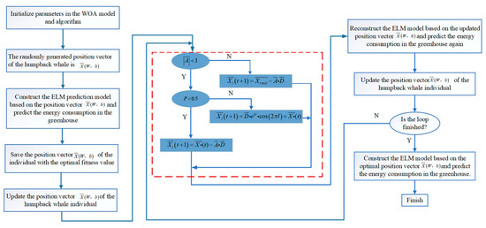
Figure 5.
Process of WOA-ELM. Add arrows to indicate a progressive relationship.
- (1)
- Determine the number of nodes in the Extreme Learning Machine network and the parameters to be optimized;
- (2)
- Initialize the WOA population and randomly generate a set of whale locations, each representing a combination of parameters for the ELM. These positions will be used for subsequent parameter optimization;
- (3)
- Training ELM for fitness assessment: For each whale location (i.e., each set of ELM parameters), the ELM model is trained using the training data. To evaluate the performance of the ELM model, metrics such as classification accuracy and mean square error are usually used to calculate the fitness;
- (4)
- Update the position of the whale according to the rules of the Whale Optimization Algorithm;
- (5)
- Determine whether the maximum number of iterations is reached, if not, repeat the whale position optimization, if the maximum number of iterations is reached, proceed to the next step;
- (6)
- The found optimal weights and thresholds are output to the ELM model, and then the greenhouse energy consumption prediction is performed.
4.4. Evaluation Indicators
In this study, the root mean square error, coefficient of determination and average absolute error are used to evaluate the prediction and measurement results. The root mean square error is used to measure the deviation between the predicted value and the measured value, and the smaller the value, the better the simulation effect. The coefficient of determination is used to measure the degree of linear correlation between two sets of data, and a value close to 1 means that the correlation between the simulated and predicted values is higher. Mean absolute error is the absolute value of the deviation of the data, the smaller the value, the better the simulation effect. The corresponding formula is as follows:
where represents the number of samples; represents the model predictions and represents the actual observations.
5. Results and Analysis
In order to fully verify the improvement effect of the WOA-ELM model constructed in this study compared with the ELM model and several typical deep learning models widely used in existing studies in the prediction of greenhouse energy consumption, this study compares and analyzes the accuracy of greenhouse energy consumption prediction of the WOA-ELM model with that of four commonly used deep learning models, namely, artificial neural network, RBF neural network, and the ELM model, under different weather conditions. The accuracy of the WOA-ELM model was compared and analyzed with four currently used deep learning models: artificial neural network, RBF neural network and ELM model under different weather conditions.
5.1. Model Parameter Setting
In the sensitivity analysis, the input variables were determined to be the factors affecting the operation of the control equipment related to the greenhouse, which were outdoor temperature, total outdoor solar radiation, total indoor solar radiation, indoor humidity, indoor temperature, and rear wall temperature. The output variables were the greenhouse power consumption, in which only the power consumption of the heaters was considered during the monitoring process, taking into account the fact that the roller shutters and skylights, as short-time operating devices, had negligible power consumption compared to the heaters. After determining the input and output variables of the model, the network parameters are configured through continuous adjustment and experimentation during the model running process, and because too many iterations will affect the training efficiency of the model, and the adaptability curve does not change much after iteration, the transfer function of the model and the related parameter values are finally selected: the number of nodes of the implicit layer is 50, the number of iterations is 50, and the number of populations is 6. Table 4 shows the model parameter partially tuned. experimental table.
Table 4.
Experimental table of partial tuning of model parameters.
To validate the effectiveness of WOA-ELM in greenhouse energy consumption forecasting, this study utilized a dataset comprising 964 observational samples from steel-framed solar greenhouses without rear slopes in the northern foothills of the Tianshan Mountains, Xinjiang. The dataset covers periods characterized by low sunlight and low temperatures in the region, encompassing three typical weather patterns: clear, cloudy, and snowy. Data collection coincided with the tomato fruiting stage—a phenological period highly sensitive to environmental temperature control with significantly higher energy demands than other growth cycles. The interannual stability of energy consumption during fruit maturation ensured the temporal representativeness of the samples. The data was divided into training and test sets at a 5:1 ratio, with the training set used for model parameter optimization and the test set for evaluating prediction accuracy. To assess the model’s generalization capability, 5-fold cross-validation was performed on 962 time series data points. The validation results are shown in Figure 6. Results indicate: the model achieved an average root mean square error of 0.544, with standard deviations of RMSE across folds < 0.7. This demonstrates the model’s robust stability in handling complex time series data without significant overfitting. The overall prediction flowchart is illustrated in Figure 7.
Figure 6.
Five-fold cross-validation RMSE plot.
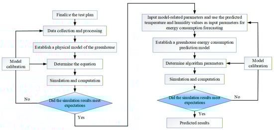
Figure 7.
Flowchart for predicting greenhouse energy consumption based on WOA-ELM algorithm. Add arrows to indicate a progressive relationship.
5.2. Analysis of Model Prediction Results
To validate the predictive accuracy of the WOA-ELM model, this study selected artificial neural networks, RBF neural networks, and unoptimized ELM models as baseline comparison models. A standardized hyperparameter optimization process ensured fairness in comparison: the BP model employed grid search to optimize learning rate, number of hidden layer nodes, and iteration count. RBF models employed Bayesian optimization to determine radial basis function width and hidden layer node count. Both ELM and WOA-ELM models uniformly targeted minimization of validation set RMSE to optimize core parameters like hidden layer node count. All models shared the identical dataset of 964 samples with a 10 min prediction step. Comprehensive evaluation metrics including MAE, RMSE, and R2 were compared, with analyses conducted for distinct weather conditions: The overcast prediction period spans from after curtain opening on 9 December 2024, to before curtain opening on 10 December 2024. The clear-sky prediction period covers from after curtain opening on 10 December 2024, to before curtain opening on 11 December 2024. Corresponding outdoor climate conditions are illustrated in Figure 8.

Figure 8.
Outdoor climatic conditions.
From Figure 9 and Figure 10, we can see that the predicted values of energy consumption in the greenhouse simulated by the four models to establish the energy consumption prediction model are more in line with the change curve of the measured values, and the change trend is consistent. Under sunny conditions, the total acceptable solar radiation is high, and the indoor temperature during the day can reach the appropriate conditions for crop growth, so the heaters are not started; under cloudy conditions, the acceptable solar radiation is weak, and the indoor temperature during the day cannot reach the appropriate conditions for crop growth, so the heaters start to work when the indoor air temperature is lower than 11 °C, and after reaching the set value, the heaters stop working. At night, the indoor temperature of the room could not reach the suitable requirements, so the heaters worked under both weather conditions. A total of 203.1 kW-h of electricity was consumed under cloudy conditions and 126.6 kW-h under sunny conditions, which shows that the intensity of the total solar radiation directly affects the level of energy consumption in greenhouses, so reasonable greenhouse management strategies and effective energy consumption prediction models can help optimize the energy consumption and ensure that the crops are grown in different weather conditions, while reducing energy consumption.
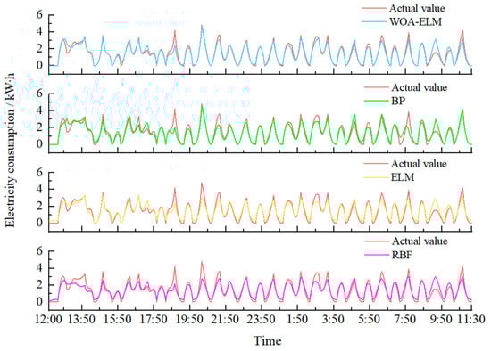
Figure 9.
Plot of the predicted changes in energy consumption in the greenhouse under cloudy conditions.
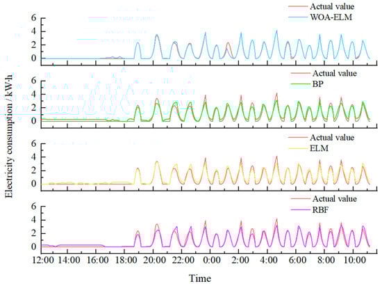
Figure 10.
Plot of the predicted changes in energy consumption in the greenhouse under sunny conditions.
Table 5 shows that under cloudy conditions, the WOA-ELM, BP, RBF, and ELM models predicted root mean square errors of 0.423, 0.585, 0.63, and 0.573, respectively, with mean absolute errors of 0.252, 0.444, 0.504, and 0.348, and linear fits of 0.93, 0.85, 0.85, and 0.88, respectively; and under sunny conditions, the WOA-ELM, BP, RBF, and ELM models predicted root mean square errors of 0.27, 0.705, 0.726, and 0.639, respectively, with mean absolute errors of 0.063, 0.477, 0.453, and 0.339, respectively, and linear fits of 0.96, 0.89, 0.88, and 0.91, respectively. the WOA-ELM model showed higher prediction under both cloudy and clear sky conditions under both cloudy and sunny conditions, indicating its adaptability to different weather conditions. The measured and simulated values of greenhouse energy consumption simulated by the ELM network model were compared with the WOA-ELM network model, and the WOA-ELM network model predicted the energy consumption with small error and high degree of fit, which was due to the optimization of the parameters of the ELM model by the WOA, so that it could better capture the dynamic change law of greenhouse energy consumption. Through the above results, it can be concluded that the order of the prediction effect of the four models from good to poor is WOA-ELM, ELM, BP, RBF. In summary, through the comparison of the coefficient of determination, root mean square error and average absolute error, it is concluded that the WOA-ELM model constructed in this study has a higher prediction accuracy, and it can predict the greenhouse energy consumption more accurately. In practical applications, the operation strategies of greenhouse heating, ventilation and irrigation equipment can be dynamically adjusted according to the prediction results of the WOA-ELM model, so as to minimize energy consumption and reduce production costs under the premise of ensuring crop growth. In addition, the WOA-ELM model can also be used for long-term trend analysis of greenhouse energy consumption, providing data support for greenhouse design and energy planning.
Table 5.
Experimental table of partial tuning of model parameters.
6. Discussion
This study constructed a physical model of the greenhouse based on the principle of heat balance. By analyzing the energy exchange process inside and outside the greenhouse, the mapping relationship between key input variables such as outdoor temperature, solar radiation, and indoor humidity and greenhouse energy consumption was clarified. Sensitivity analysis results show that parameters including indoor temperature, total outdoor solar radiation, and outdoor temperature have the most significant impacts on energy consumption, providing a mechanistic basis for subsequent model construction. The following discussion focuses on the model optimization strategy, its performance versus traditional models under different weather, practical application value, and current limitations with future improvements.
- (1)
- To address the issues of high energy consumption in solar greenhouses and the difficulty of achieving optimal selection of hyperparameters in a single Extreme Learning Machine (ELM), this study introduced the Whale Optimization Algorithm (WOA), an intelligent algorithm, to optimize the parameters of ELM for improved prediction accuracy. By optimizing weights and thresholds, the impact of randomness in parameter selection was reduced, making the model more consistent and stable across different runs. A comparative analysis of the prediction performance of the WOA-ELM network model with Artificial Neural Network (ANN), Radial Basis Function (RBF) neural network, and ELM model revealed differences in model errors under varying weather conditions. On cloudy days, solar radiation is negligible, and the thermal load is almost entirely borne by the heat fan. Energy consumption is mainly driven by the indoor-outdoor temperature difference, showing an approximate linear relationship that is easily identifiable by each model, resulting in overall lower errors. On sunny days, solar radiation increases sharply, leading to a strong coupled nonlinear relationship among solar radiation energy, indoor ventilation heat loss, and crop latent heat. Indoor ventilation heat loss is highly sensitive to skylight opening, wind speed, and transpiration latent heat, resulting in generally higher model errors on sunny days. Error comparison results indicate that under different weather conditions, the WOA-ELM network model exhibits higher prediction accuracy in terms of both fitting degree and the error between predicted and actual values. It can better capture nonlinear transient changes in the greenhouse, further demonstrating its robustness and accuracy advantages in complex light-temperature environments. This model provides an accurate method for greenhouse energy consumption prediction, management, and control, with significant practical significance and value.
- (2)
- Solar greenhouses in the northern slope of the Tianshan Mountains in Xinjiang require substantial heat supplementation for safe overwintering production, leading to increased energy consumption and production costs. The model constructed in this study provides a scientific basis for the design of winter heating systems. Based on this model, an optimized heating control strategy can be proposed: using sensors and controllers to real-time monitor parameters such as temperature, humidity, and light inside and outside the greenhouse, and automatically controlling the switch and power of heating equipment according to preset control strategies. This approach enables precise temperature control, reducing energy consumption and costs to a certain extent.
- (3)
- The currently constructed WOA-ELM solar greenhouse energy consumption prediction model achieves high-precision prediction under sunny and cloudy conditions and clarifies the sources of errors, but it still has limitations. The samples only cover the tomato fruiting stage, failing to consider the impact of changes in leaf area index and canopy heat transfer coefficient during the seedling and flowering stages on the heat balance, which may increase the prediction error of the model by 15–20% during other growth stages. Additionally, the model’s adaptability to extreme weather conditions such as cold waves and heavy snow remains unvalidated, and such weather may increase the model’s RMSE to above 0.6. Future research can improve the model by incorporating a dynamic parameter module for crop growth stages, constructing specialized sub-models for extreme weather, and adjusting the weights of heat transfer and heat dissipation terms in the heat balance equation.
7. Conclusions
- (1)
- Under cloudy conditions, the root mean square errors (RMSEs) of the WOA-ELM, BP, RBF, and ELM models are 0.423, 0.585, 0.63, and 0.575, respectively; the mean absolute errors (MAEs) are 0.252, 0.444, 0.504, and 0.348, respectively; and the coefficients of determination (R2) are 0.93, 0.85, 0.85, and 0.88, respectively. Under sunny conditions, the RMSE values of the above four models are 0.27, 0.705, 0.726, and 0.639, respectively; the MAE values are 0.063, 0.477, 0.453, and 0.339, respectively; and the R2 values are 0.96, 0.89, 0.88, and 0.91, respectively. The ranking of the prediction performance of the four models from best to worst is WOA-ELM > ELM > BP > RBF.
- (2)
- By integrating the mechanistic analysis of the physical model and the parameter optimization of the intelligent algorithm, the WOA-ELM model achieves higher prediction accuracy under different weather conditions, verifying its effectiveness in solar greenhouse energy consumption prediction.
- (3)
- The model provides a theoretical basis for the energy load design, management, and control of steel-frame solar greenhouses without back slopes in the northern slope of the Tianshan Mountains in Xinjiang. Based on its prediction results, the operation strategies of greenhouse heating, ventilation, and irrigation equipment can be dynamically adjusted to minimize energy consumption and reduce production costs while ensuring crop growth. Additionally, the WOA-ELM model can be used for long-term trend analysis of greenhouse energy consumption, providing data support for greenhouse design and energy planning.
Author Contributions
Conceptualization, W.Z.; data curation, C.X.; formal analysis, C.X.; funding acquisition, W.Z.; investigation, J.C.; methodology, C.X.; project administration, Y.D.; resources, N.L.; software, C.X.; Supervision, Y.T.; validation, C.X.; visualization, C.X.; writing—original draft, C.X.; writing—review & editing, W.Z. wrote the paper. All authors have read and agreed to the published version of the manuscript.
Funding
Research on Key Technologies for High-efficiency Utilization of Solar Energy and Intelligent Management of Greenhouses in Desert Area, 2023B02020, Project of science and Technology assistance program for Xinjiang, Research and Application of Key Products of Dual-Effect Solar Energy for Heating and Dehumidification in Solar Greenhouses, 2025E02028, and Project of key fund project of Research on Energy Consumption Optimization for Environmental Regulation of Greenhouse based on Solar Heating and Cooling Dual Supply and Multi-Agent System, 2025D01D22.
Institutional Review Board Statement
Not applicable.
Informed Consent Statement
Not applicable.
Data Availability Statement
The data presented in this study are available upon request from the corresponding author. The data are not publicly available as the device is in the research and development stage; it needs to be further studied and improved.
Conflicts of Interest
The authors declare no conflict of interest.
References
- Hassanien, R.H.E.; Li, M.; Lin, W.D. Advanced applications of solar energy in agricultural greenhouses. Renew. Sustain. Energy Rev. 2016, 54, 989–1001. [Google Scholar] [CrossRef]
- Zhu, C.; He, Q.; Zhao, Z.; Liu, X.; Pu, Z. Comparative Analysis of Ozone Pollution Characteristics between Urban Area and Southern Mountainous Area of Urumqi, China. Atmosphere 2023, 14, 1387. [Google Scholar] [CrossRef]
- Kaneda, Y.; Ibayashi, H.; Oishi, N.; Mineno, H. Greenhouse environmental control system based on SW-SVR. Procedia Comput. Sci. 2015, 60, 860–869. [Google Scholar] [CrossRef]
- Cunha, J.B.; Couto, C.; Ruano, A.E.B. Real-time parameter estimation of dynamic temperature models for greenhouse environmental control. Control Eng. Pract. 1997, 5, 1473–1481. [Google Scholar] [CrossRef]
- Li, S.J.; Wu, L.X.; Wang, Y.T.; Geng, T.; Cai, W.J.; Gan, B.L.; Jing, Z.; Yang, Y. Intensified Atlantic multidecadal variability in a warming climate. Nat. Clim. Change 2025, 15, 1–8. [Google Scholar] [CrossRef]
- Jolliet, O.; Danloy, L.; Gay, J.-B.; Munday, G.; Reist, A. HORTICERN: An improved static model for predicting the energy consumption of a greenhouse. Agric. For. Meteorol. 1991, 55, 265–294. [Google Scholar] [CrossRef]
- Singh, R.D.; Tiwari, G.N. Energy conservation in the greenhouse system: A steady state analysis. Energy 2010, 35, 2367–2373. [Google Scholar] [CrossRef]
- Ahamed, M.S.; Guo, H.; Tanino, K. Development of a thermal model for simulation of supplemental heating requirements in Chinese-style solar greenhouses. Comput. Electron. Agric. 2018, 150, 235–244. [Google Scholar] [CrossRef]
- Dai, J.; Luo, W.; Li, Y. A microclimate model-based energy consumption prediction system for greenhouse heating. Sci. Agric. Sin. 2006, 11, 21. [Google Scholar]
- Xu, F.; Zhang, L.B.; Chen, J.L.; Zhan, H.W. Modeling and simulation of subtropical greenhouse microclimate in China. Nongye Jixie Xuebao = Trans. Chin. Soc. Agric. Mach. 2005, 36, 102–105. [Google Scholar]
- Shen, Y.; Wei, R.; Xu, L. Energy consumption prediction of a greenhouse and optimization of daily average temperature. Energies 2018, 11, 65. [Google Scholar] [CrossRef]
- Wang, X. Simulation of Microclimate and Energy Consumption Prediction in Modern Greenhouses in Southern China; Nanjing Agricultural University: Nanjing, China, 2003. [Google Scholar]
- Dai, J.; Luo, W.; Li, Y.; Qiao, X.; Wang, C. Research on Greenhouse Energy Consumption Prediction System Based on Microclimate Model. Sci. Agric. Sin. 2006, 39, 6. [Google Scholar]
- Yao, Y.; Dai, J.; Luo, W.; Su, G. Simulation of Energy Consumption Distribution for Year-Round Cucumber Production in Multi-Span Greenhouses in China. Trans. Chin. Soc. Agric. Eng. 2011, 27, 273–279+395. [Google Scholar]
- Ho, L.; Jerves-Cobo, R.; Forio, M.A.E.; Mouton, A.; Nopens, I.; Goethals, P. Integrated mechanistic and data-driven modeling for risk assessment of greenhouse gas production in an urbanized river system. J. Environ. Manag. 2021, 294, 112999. [Google Scholar] [CrossRef]
- Li, Z.; Wang, P.; Zhang, J.; Mu, S. A strategy of improvingindoor air temperature prediction in HVAC system based onmultivariate transfer entropy. Build. Environ. 2022, 219, 109164. [Google Scholar] [CrossRef]
- Liu, R.; Li, M.; Guzmán, J.L.; Rodríguez, F. A fast and practical one-dimensional transient model for greenhouse temperature and humidity. Comput. Electron. Agric. 2021, 186, 106186. [Google Scholar] [CrossRef]
- Taki, M.; Ajabshirchi, Y. Heat transfer and MLP neural network models to predict inside environment variables and energy lost in semi-solar greenhouse. Energy Build. 2015, 110, 314–329. [Google Scholar] [CrossRef]
- Trejo-Perea, M.; Herrera-Ruiz, G.; Rios-Moreno, J.; Miranda, R.C.; Rivasaraiza, E. Greenhouse energy consumption prediction using neural networks models. Training 2009, 1, 2. [Google Scholar]
- De Zwart, H.F. Analzing Energy-Saving Options in Greenhouse Cultivation Using a Simuation Model. Ph.D. Dissertation, Agricutural University of Wageningen, Wageningen, The Netherlands, 1996. [Google Scholar]
- Khoshnevisan, B.; Rafiee, S.; Omid, M.; Yousefi, M.; Movahedi, M. Modeling of energy consumption and GHG (greenhouse gas) emissions in wheat production in Esfahan province of Iran using artificial neural networks. Energy 2013, 52, 333–338. [Google Scholar] [CrossRef]
- Özden, S.; Dursun, M.; Aksöz, A.; Saygın, A. Prediction and modelling of energy consumption on temperature control for greenhouses. Politek. Derg. 2019, 22, 213–217. [Google Scholar] [CrossRef]
- Chen, J.; Chen, J.; Yang, J.; Xu, F.; Shen, Z. Energy consumption prediction of semi-closed greenhouses based on self-accelerating genetic particle swarm optimization algorithm. Trans. Chin. Soc. Agric. Eng. 2015, 31, 186–193. [Google Scholar]
- Zhang, Y.; Lin, S.; Shen, J.; Chen, C.; Li, Z.; Xie, T. Energy consumption prediction model for multi-span greenhouses based on LSTM. Tianjin Agric. Sci. 2023, 29, 74–79. [Google Scholar]
- Zhang, Y.; Zhang, Y.; Cheng, R.; Wang, C. Prediction of heat release from the walls of solar greenhouses based on partial least squares regression. Jiangsu Agric. Sci. 2022, 50, 208–213. [Google Scholar]
- Zhang, G. Research on Greenhouse Adaptive Control System Based on T-S Fuzzy Neural Network; Taiyuan University of Technology: Taiyuan, China, 2019. [Google Scholar]
- Liu, H. Research on the Water Demand Law of Greenhouse Tomato and the Index of High-Quality and High-Efficiency Irrigation; Chinese Academy of Agricultural Sciences: Beijing, China, 2010. [Google Scholar]
- Liao, S.; Feng, C. Meta-ELM: ELM with ELM hidden nodes. Neurocomputing 2014, 128, 81–87. [Google Scholar] [CrossRef]
- Kumar, M.; Gouw, M.; Michael, S.; Sámano-Sánchez, H.; Pancsa, R.; Glavina, J.; Diakogianni, A.; Valverde, J.A.; Bukirova, D.; Čalyševa, J.; et al. ELM—The eukaryotic linear motif resource in 2020. Nucleic Acids Res. 2020, 48, D296–D306. [Google Scholar] [CrossRef]
- Lei, X.; Xu, X.; Zhou, S. Potato Yield Prediction Research Based on Improved Artificial Neural Networks Using Whale Optimization Algorithm. Potato Res. 2024, 68, 1717–1726. [Google Scholar] [CrossRef]
- Monteiro, D.K.; Miguel, L.F.F.; Zeni, G.; Becker, T.; de Andrade, G.S.; de Barros, R.R. Whale Optimization Algorithm for structural damage detection, localization, and quantification. Discov. Civ. Eng. 2024, 1, 98. [Google Scholar] [CrossRef]
- Mostafa Bozorgi, S.; Yazdani, S. IWOA: An improved whale optimization algorithm for optimization problems. J. Comput. Des. Eng. 2019, 6, 243–259. [Google Scholar] [CrossRef]
- Liu, Z.; Huang, X.; Wang, X. PM2.5 prediction based on modified whale optimization algorithm and support vector regression. Sci. Rep. 2024, 14, 23296. [Google Scholar] [CrossRef] [PubMed]
- Chen, W.; Hong, H.; Panahi, M.; Shahabi, H.; Wang, Y.; Shirzadi, A.; Pirasteh, S.; Alesheikh, A.A.; Khosravi, K.; Panahi, S.; et al. Spatial prediction of landslide susceptibility using gis-based data mining techniques of ANFIS with whale optimization algorithm (WOA) and grey wolf optimizer (GWO). Appl. Sci. 2019, 9, 3755. [Google Scholar] [CrossRef]
- Li, C.; Zhou, J.; Khandelwal, M.; Zhang, X.; Monjezi, M.; Qiu, Y. Six novel hybrid extreme learning machine–swarm intelligence optimization (ELM–SIO) models for predicting backbreak in open-pit blasting. Nat. Resour. Res. 2022, 31, 3017–3039. [Google Scholar] [CrossRef]
- Huang, G.B.; Wang, D.H.; Lan, Y. Extreme learning machines: A survey. Int. J. Mach. Learn. Cybern. 2011, 2, 107–122. [Google Scholar] [CrossRef]
- Zhou, W.; Xie, C.; Dong, Y.; Gao, Y.; Tang, Y. Comparative Testing and Analysis of Winter Microclimate in Solar Greenhouses in Urumqi Region. J. Shenyang Agric. Univ. 2024, 55, 483–489. [Google Scholar]
Disclaimer/Publisher’s Note: The statements, opinions and data contained in all publications are solely those of the individual author(s) and contributor(s) and not of MDPI and/or the editor(s). MDPI and/or the editor(s) disclaim responsibility for any injury to people or property resulting from any ideas, methods, instructions or products referred to in the content. |
© 2025 by the authors. Licensee MDPI, Basel, Switzerland. This article is an open access article distributed under the terms and conditions of the Creative Commons Attribution (CC BY) license (https://creativecommons.org/licenses/by/4.0/).