A Digital Twin Framework for Sensor Selection and Microclimate Monitoring in Greenhouses

Abstract

Digital twins, defined as virtual counterparts of physical systems that evolve with sensor data have potential applications in controlled-environment agriculture. This study previews the integration of adaptive Microclimate Monitoring within a Unity-based digital twin of a strawberry greenhouse to support dynamic sensor selection and reallocation. Using data collected from 56 distributed temperature–relative humidity sensors, a Thompson Sampling algorithm was deployed to assign monthly importance rankings and identify season-specific subsets of sensors. To evaluate how well these subsets represented the whole sensor network, we used the Z-index, which measures distributional consistency. Across all observed months, Z-index values remained close to zero, with values of 0.037 in February, 0.012 in April, −0.002 in June, and 0.025 in October for relative humidity. These results indicate that the digital twin framework sustains the overall climate trend while reducing sensing redundancy, pointing to its potential role in future climate monitoring strategies within greenhouse systems.

1. Introduction

The increasing demand for sustainable agriculture necessitates advanced technological solutions, particularly in controlled environments like greenhouses [1,2]. Implementing digital twins in greenhouse horticulture represents a cyber–physical approach to Greenhouse management [3]. A digital twin is a virtual counterpart of a physical object, Asset, process, or system that reproduces its structure and measurable states. Depending on the application, the twin may remain static, supporting offline diagnostics, or update dynamically as new sensor data is retrieved. In greenhouse agriculture, such models provide a unified platform for monitoring key environmental parameters, including air temperature, relative humidity, dewpoint temperature, humidity ratio, specific volume, and moist-air enthalpy. By incorporating these variables into a single representation, digital twins facilitate high-fidelity simulations and continuous microclimate assessment [4,5]. Digital Twin has three major components: a physical product, a virtual representation of that product, and the bi-directional data connections that transmit data from the physical product to the virtual representation, as well as information and processes from the virtual representation to the physical product. While digital twins have seen widespread adoption across industries, including manufacturing, smart cities, and healthcare, their use in adaptive environmental Monitoring, particularly in agriculture, remains limited [4,6,7]. Digital twin (DT) technology has great potential to cause a paradigm shift in agriculture by enabling intelligent automation, optimizing resource use, and enhancing productivity [8]. DTs in agriculture facilitate the virtual analysis of soil, climate, yield, and plant data, leading to increased yields [9,10,11].

Despite the growing use of digital twins in various domains, many existing frameworks are static, relying on fixed sensor configurations that do not adapt to dynamic conditions in cyber–physical environments. To address this, we present a general-purpose, reinforcement learning-driven digital twin framework that dynamically selects informative sensor locations over time. A Virtual 3D model of the Greenhouse, developed in Unity, mirrors the spatial layout and sensor distribution of the physical environment. Employing Thompson Sampling, a Bayesian reinforcement learning algorithm, the system dynamically identifies the most informative sensor locations over time. A Strawberry Greenhouse serves as a representative testbed for validating our proposed Digital twin framework, due to its high sensitivity to environmental changes and the need for efficient sensor placement. Strawberries are well-suited for greenhouse cultivation due to the numerous advantages of controlled environments. Cultivating strawberries in a greenhouse is beneficial, particularly for farmers seeking to produce fresh berries throughout the year [12,13]. The controlled environment of a greenhouse facilitates year-round harvests, including during winter, thereby enabling the continuous availability of high-quality strawberries irrespective of external climatic conditions [14]. The greenhouse setting effectively shields plants from adverse weather conditions, such as frost, excessive rainfall, or extreme heat, thereby controlling and improving the growing environment [15].

Although strawberry greenhouses are used as a case study in this work, the proposed digital twin framework is domain-agnostic and applicable to a broad range of cyber–physical systems requiring dynamic sensing strategies. This approach improves monitoring efficiency, reduces sensor data redundancy, and enables climate-responsive decision support for precision greenhouse management. The key contributions of this work are as follows:

(1)

A digital twin of a strawberry greenhouse was developed using Unity to create a 3D virtual environment that mirrors the physical layout, plant beds, and sensor positions.

(2)

The digital twin was integrated with sensor data capturing temperature and relative humidity from 56 distributed locations to enable continuous environmental Monitoring.

(3)

A reinforcement learning algorithm based on Thompson Sampling was employed to select the most informative sensor locations over time adaptively.

(4)

The accuracy of the selected sensor subsets was validated against the whole network using the Z-index, the Mean Absolute Error(MAE), and Root Mean Squared Error (RMSE).

(5)

An interactive interface combining a graphical user interface (GUI) and 3D visualization was implemented to support immersive user interaction and temporal queries.

2. Related Works

2.1. Optimal Sensor Placement in a Greenhouse

Sensor placement in greenhouses is crucial for ensuring effective environmental Monitoring and optimal resource utilization in crop cultivation. The approach focuses on determining the sensor that captures the unique microclimate within the Greenhouse with the least data redundancy. Greenhouses rely on sensors to measure key environmental parameters such as temperature, relative humidity, light intensity, soil moisture, and CO₂ concentration, which directly or indirectly affect plant growth. The strategic placement of these sensors is essential for capturing the spatial variability of measured variable parameters within the greenhouse microclimate and providing reliable data for agricultural systems. Poor sensor placement can lead to inaccurate readings, inefficient climate control, and suboptimal growing conditions, impacting crop productivity and energy efficiency [11,16].

Determining optimal sensor locations often involves analyzing greenhouse geometry, air circulation patterns, and crop density to ensure comprehensive Monitoring. Advanced computational techniques, such as simulation-based methods, reinforcement learning, and machine learning algorithms, are increasingly employed to identify the most effective sensor placements. These technologies help minimize redundancy, ensuring that the data collected accurately represents environmental conditions across the Greenhouse [17,18]. Several studies have investigated sensor placement strategies in greenhouses, aiming to optimize environmental Monitoring. The objective for optimization using a data-driven approach often centers around selecting a sensor with the least redundancy or sensors of the closest proximity to the centroid within a cluster of sensors. For example, [16] studied optimizing sensor locations in protected cultivation systems using grid search methods to attain the lowest root mean squared error (RMSE) in temperature and relative humidity predictions. The research highlighted the importance of evenly distributed sensors in capturing spatial variability and reducing the risk of localized inaccuracies. Ajani et al. (2023) [19] developed a genetic programming approach for optimal sensor placement in greenhouses by modeling aggregated reference microclimate data. Their method identified a symbolic regression model that selected the minimum number of sensors (8) necessary to estimate temperature and relative humidity for monitoring and control purposes across multiple months.

Lee et al. (2019) [20] evaluated optimal sensor placements in an eight-span greenhouse by comparing all possible combinations of sensor locations using error- and entropy-based methods. Their approach selected locations that best matched average conditions or were most sensitive to external environmental variations, thereby supporting uniform ecological Monitoring and control. Ferentinos et al. [21] deployed a wireless sensor network in a commercial greenhouse to map the spatial variation in microclimate conditions, specifically temperature, relative humidity, leaf temperature, and radiation intensity. Their measurements revealed significant microclimate gradients, with temperature and relative humidity demonstrating clear spatial heterogeneity influenced by structural features and solar radiation exposure. These variations underscore that assuming a uniform greenhouse environment can mask critical localized differences, which are essential for precision monitoring and climate control in controlled environment agriculture.

Uyeh et al. (2022) [22] proposed an online machine learning-based clustering method using K-Means++ to group greenhouse sensors based on derived air properties such as Enthalpy and specific volume. This study utilized sensor data collected over multiple months to identify optimal sensor locations. It selected representative sensors from heterogeneous clusters by using Euclidean distance to cluster centroids. Pylianidis et al. [11] reviewed machine learning and spatial analysis methods to determine optimal sensor configurations. Their study demonstrated that strategically placed sensors enhance the efficiency of irrigation and climate control systems while reducing energy consumption. Similarly, [18] Purcell et al. explored sensor clustering techniques to identify key zones within the Greenhouse for monitoring critical parameters.

In this study, we adopted the reinforcement-learning approach described in [23] to demonstrate a cyber–physical method for adapting the sensing infrastructure to seasonal variability in a protected-cultivation system. This approach was chosen because it employs Bayesian inference to identify informative sensors while requiring less data than alternative methods. All together, these studies highlight advancements in sensor placement methodologies, from conventional grid-based approaches to modern machine learning and simulation-driven techniques. A step forward from the analysis presented in the reviewed literature above would be the demonstration and evaluation of the application of optimal sensor placement methodology within a simulation infrastructure using cyber–physical approaches.

2.2. Digital Twin Applications in Agriculture

As previously stated, a digital twin is a virtual replica of a physical asset that updates in real time or periodically through continuous data collected from sensors within the physical Asset. Digital Twins are applied in agriculture to improve agricultural systems’ productivity and reduce resource consumption [17]. Digital Twins have immense potential in crop and livestock management. They can be employed to virtually monitor and control the microclimate of crops and livestock and their growth in real time [17,18,24]. Digital Twins offer several advantages in agriculture, including predictive analytics and real-time monitoring capabilities, all while operating in an immersive virtual environment to support decision-making with added spatial context. Digital Twins are primarily used as simulations, allowing farmers to simulate different scenarios or decisions (what-if analysis) while using fewer resources, guided by simulation-based predictions. This helps farmers to visualize potential outcomes to make the best decisions for their farms [11]. Digital twins are also employed within agricultural supply chains. Post-harvest, perishable goods encounter various climates and conditions as they transit from farm to fork. Digital twins can monitor and provide detailed information on these conditions through simulations, enabling the design of preventive measures to maintain food quality and reduce losses [25]. Ghandar et al. integrate real-time, sensor-calibrated aquaponics simulations with a city-scale agent-based optimizer to show that a digital-twin decision-support system can accurately steer local operations and boost the urban share of fresh produce to ~65%, underscoring its scalability for coordinated urban agriculture [26,27].

Spyrou et al. [28] examine the use of Virtual Reality-based Digital Twins (DTs) for pharmaceutical cannabis production. Their design-oriented approach applies established architectural frameworks to model complex, regulated cultivation environments. The authors developed a VR prototype linked to live sensor data, enabling remote Monitoring and interaction. While focused on cannabis, their framework is broadly applicable to controlled-environment agriculture. Another study by Chaux et al. [17] provided a DT framework and architecture, controlled environment demonstration with a case study on the use of integrated Internet of Things (IoT) sensors with digital twins to monitor greenhouse conditions, demonstrating their usefulness in crop management through microclimate monitoring. The authors emphasized the role of virtual simulations in testing sensor locations before implementation, which reduces trial-and-error efforts in physical greenhouses.

Ko et al. [29] present the development of a Digital Twin platform tailored for vertical farming environments. The system integrates real-time data acquisition, environmental control, and simulation capabilities to enhance operational efficiency and crop management. By leveraging Internet of Things technologies and advanced modeling techniques, the platform enables precise Monitoring and control of key parameters, including temperature, relative humidity, and lighting. The implementation demonstrates the potential of DTs in optimizing resource usage and improving yield outcomes in controlled agricultural settings. From the reviewed literature (see

Table 1. A comparative literature review highlighting the unique integration of methods in this work.

Paper	Virtual Environment	Reinforcement Learning	Sensor Selection/ Optimization	Seasonal Data Collection	Cloud Storage Infrastructure
Virtual Reality-Based Digital Twins: A Case Study on Pharmaceutical Cannabis [28]
Digital twin-driven system for efficient tomato harvesting in greenhouses [24]
Virtual reality-based digital twins for greenhouses: A focus on human interaction [3]
A Decision Support System for Urban Agriculture Using Digital Twin: A Case Study with Aquaponics [26].
This paper

), one of the crucial gaps in knowledge identified relates to the Use of Digital twins for Monitoring and analyzing the effects of microclimate variation in Controlled Environment Agriculture (CEA), specifically in relation to the location or placement of sensors in the Greenhouse.

3. Materials and Methods

The research reported within this paper is based on a design-oriented methodology, which is widely applied in information technology research [30]. The approach emphasizes iterative development and refinement of innovative solutions through systematic design, implementation, and evaluation. This methodology is particularly well-suited for this work, as it integrates theoretical insights with practical applications, ensuring that the resulting digital twin framework is both theoretically sound and practically effective. Figure 1 below shows the methodology diagram adopted for this project. It outlines an approach that integrates user interface, Data Management, and reinforcement learning to establish the greenhouse digital twin. At the core of this research methodology is the Digital Environment, which serves as the foundation for integrating various technologies and processes. This environment connects the physical Greenhouse with its virtual counterpart, enabling data transfer and real-time Monitoring. The 3D virtual strawberry greenhouse, serving as the virtual counterpart of the physical Greenhouse, is developed using Unity (6000.0 LTS) and Blender (4.2 LTS). Unity was chosen for its real-time rendering performance, C# scripting and plugin ecosystem (e.g., MQTT/REST integrations for live sensor streams), Blender import pipeline, and broad support for desktop and VR.

The physical Greenhouse serves as the primary data source, where sensors continuously monitor key environmental parameters such as temperature and relative humidity, with data transmitted through a wireless network controller (Model UNWC-W-75, UBN, Daegu, Republic of Korea). Collected data is stored in a DynamoDB database, chosen for its ability to efficiently manage large volumes of time-series sensor data. Communication between the physical Greenhouse and the digital environment is handled via Node.js and AWS, ensuring secure, real-time data transmission and synchronization. The system architecture supports a bidirectional flow: data from the physical environment updates the virtual model, while insights from the virtual model can guide actions in the physical Greenhouse. The digital twin was developed in Unity 6 (6000.0 LTS) and executed on a 64-bit Windows workstation with an Intel Core i9-10900 (2.80 GHz) and 64 GB RAM, providing sufficient resources for real-time processing and visualization.

3.1. Experimental Setup: Data Collection from a Strawberry Greenhouse

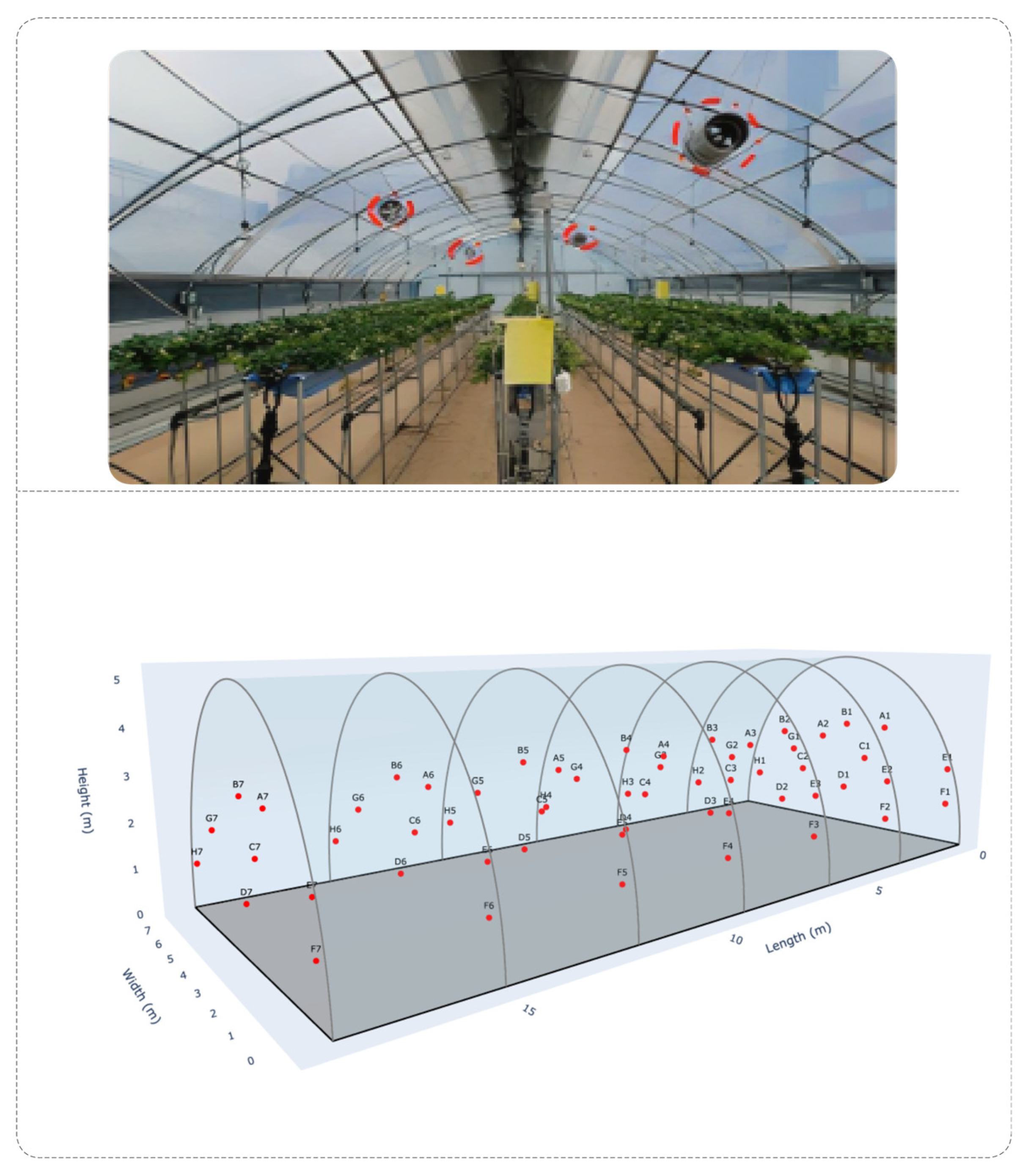
The Greenhouse selected for this study is located on the Kyungpook National University research farm in Daegu, South Korea (35°53′43.0″ N and 128°36′49.1″ E) [16]. For systematic sensor installation, sensors were positioned at 56 evenly distributed points within the Greenhouse, maintaining 1 m vertical and 3 m horizontal spacing (Figure 2). The Cartesian coordinates (XYZ) of each sensor were determined, and temperature and relative humidity readings were collected from all sensor points. The sensors were installed to ensure comprehensive environmental Monitoring based on their coverage range. Strawberry plants were grown on five beds installed at a height of 1.1 m, with each bed measuring 15 m in length and 0.26 m in width. Each bed contained 126 plants, resulting in approximately 630 strawberry plants in the experimental Greenhouse.

The psychrometric parameters used in this study were computed based on the measured air temperature, denoted as ${ T}_C$, in degrees Celsius, and the relative humidity (RH) expressed as a percentage. Four key psychrometric variables were derived from these measurements. The first is the Dew Point Temperature ($T_{ d}$ °C), which represents the temperature at which air becomes saturated with moisture and dew begins to form. The second is the Humidity Ratio ($W$, kg of water vapor per kg of dry air), which quantifies the mass of water vapor present per unit mass of dry air. The third is the Enthalpy ($h$, kJ per kg of dry air), representing the total heat content of the moist air, which accounts for both sensible heat (associated with temperature) and latent heat (associated with moisture). The fourth is the Specific Volume ($SV$, cubic meters per kg of dry air), which refers to the volume occupied by a unit mass of moist air, influenced by both temperature and relative humidity conditions. The calculations for these psychrometric variables were based on the assumption of standard atmospheric pressure, where the atmospheric pressure ($P_{atm}$) equal to 101.325 kilopascals (kPa). The saturation vapor pressure ($P_{ws}$) was first calculated using the Magnus formula, expressed as:

$$P_{ws}=A\times \exp \left({\displaystyle \frac{m\times T_C}{T_C+T_n}}\right)$$

(1)

where the constant $A$ is equal to 6.1121 hPa, $m$ is equal to 17.62 ad, and $T_n$ is equal to 243.12 degrees Celsius.

The actual vapor pressure ($P_w$) was then computed using the formula:

$$P_w=\left({\displaystyle \frac{RH}{100}}\right)\times P_{ws}$$

(2)

$$\alpha =\ln \left({\displaystyle \frac{P_w}{A}}\right)$$

(3)

$$T_d={\displaystyle \frac{T_n\times \alpha }{m-\alpha }}$$

(4)

$$W=0.622\times {\displaystyle \frac{P_w}{\left(P_{atm}\times 10\right)-P_w}}$$

(5)

$$h=1.006\times T_C+W\times \left(2501+1.86\times T_C\right)$$

(6)

$$SV={\displaystyle \frac{0.287042\times T_K\times \left(1+1.6078\times W\right)}{P_{atm}}}$$

(7)

where is the absolute temperature in Kelvin:$T_K=T_C+273.15.$

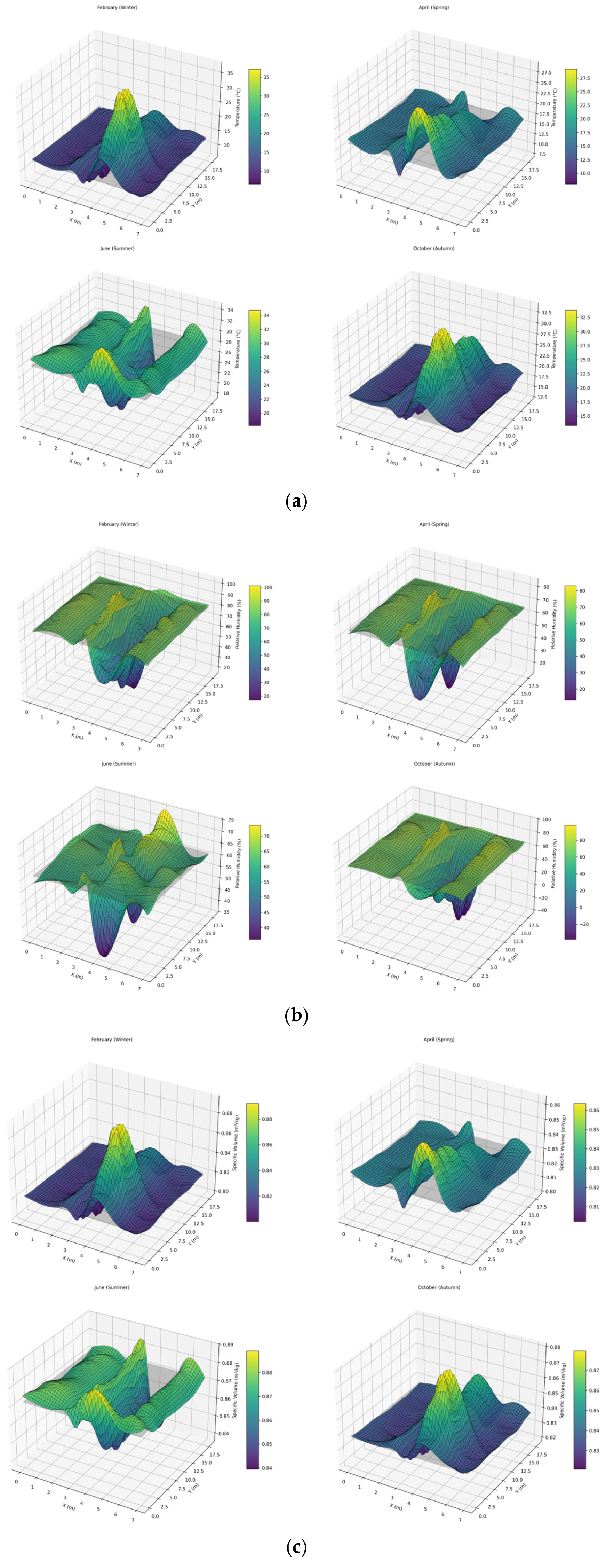
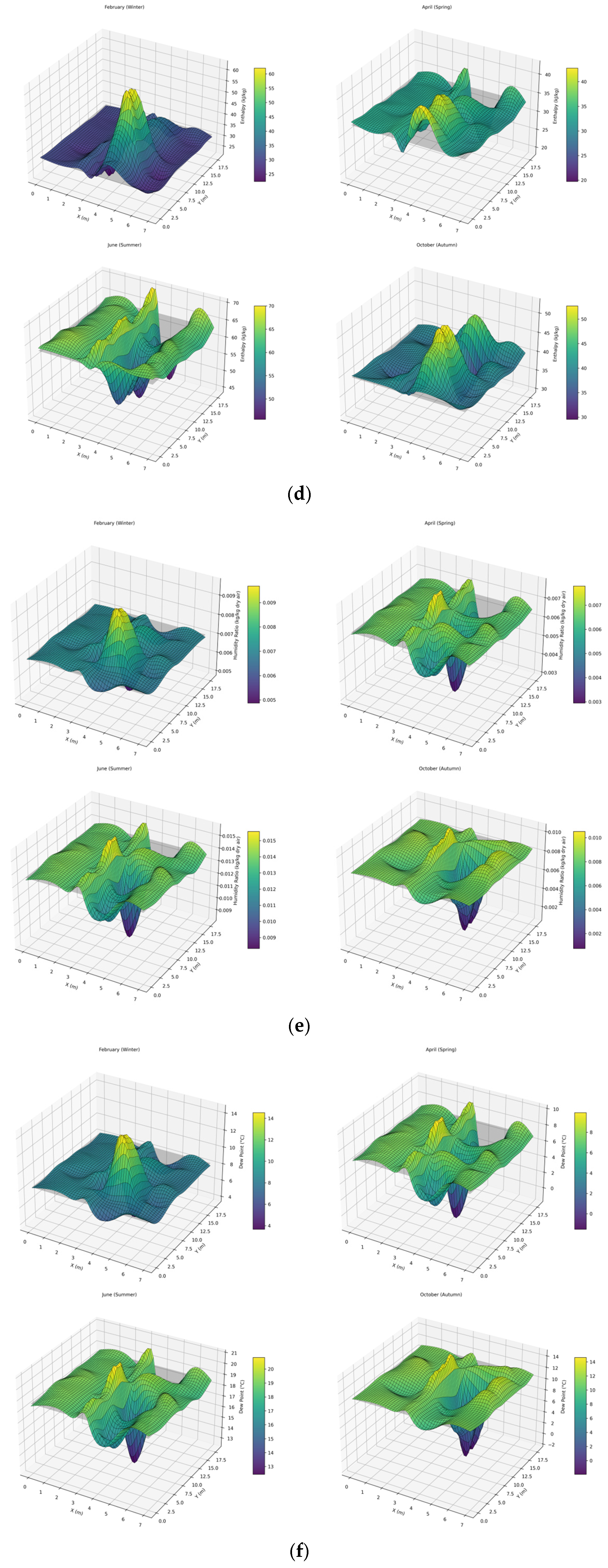
Each of the 56 sensors (see Figure 2) provided two independent readings (temperature and relative humidity) at one-minute intervals (sampling rate). The temperature sensors had a reading range between −20 °C and 80 °C, while the relative humidity sensors ranged from 0% to 100%. The sensors were specially fabricated to have similar error margins of ±0.3 °C for temperature measurements and ±2% for relative humidity measurements. They were placed in plastic protection cases to protect the sensors from direct solar radiation, which could cause inaccuracies in the readings. Additionally, the sensors were tightly installed to prevent movement. An in-house software program was developed for mobile devices to receive and save data from sensors in real-time, with the data also being backed up in the cloud. The resulting dataset is a time series in nature, comprising $n$ samples and 56 features corresponding to individual sensor locations within the Greenhouse. Data were collected across multiple months—February (Winter), March (Winter), April (Spring), May (Spring), June (Summer), July (Summer), and October (Autumn) to capture seasonal variability in the internal microclimate. Figure 3a–f presents 3D surface plots that visualize the spatial distribution of monthly mean values for selected environmental parameters. These surface plots illustrate how microclimatic conditions evolve over time, with noticeable deformations in the surface topology, such as shifting peaks and valleys, reflecting seasonal impacts.

For interpretability, a 2D horizontal plane representing the overall mean value of each parameter is superimposed on each surface plot. This plane serves as a reference, enabling clear visualization of regions within the Greenhouse that exhibit values above or below the seasonal average, commonly referred to as “mean crossings.” For instance, in cooler months such as February, central regions exhibit elevated temperatures due to localized heating, while in warmer months, higher temperatures are observed around the periphery, indicative of heat intrusion from external sources. These visual patterns underscore the importance of spatially resolved sensing for effective greenhouse monitoring and control.

3.2. Sensor Data Management

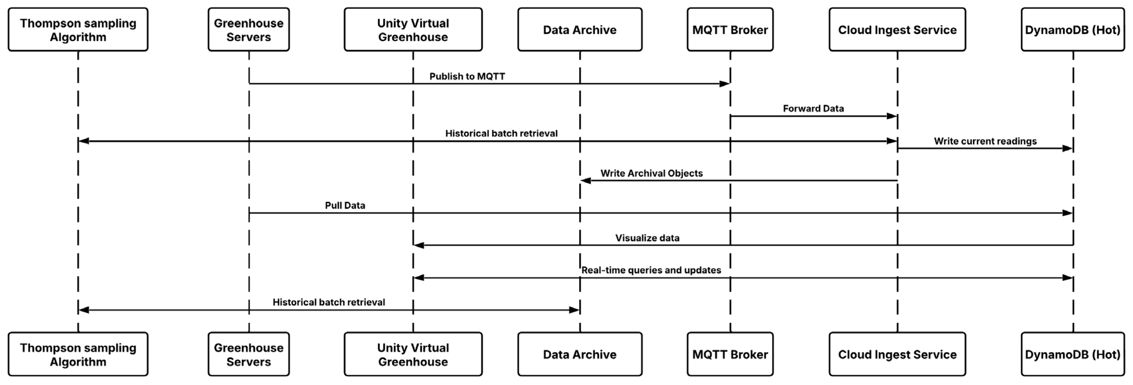
Sensor readings for temperature and relative humidity are sent from the Greenhouse over the lightweight publish–subscribe network protocol designed for Internet of Things (IoT) communication, MQTT, whose headers are optimized to minimize network bandwidth while sending each sensor’s readings, including the sensor ID and timestamp [31]. Messages are sent to the project’s MQTT broker, a node dedicated to buffering and forwarding traffic; its sole purpose is reliable routing, not storage. A cloud ingest service then validates the payload, adds metadata such as the device’s calibration profile, and writes the data to two complementary stores [32]. Amazon DynamoDB serves as the hot store: its role is to keep the most recent, time-ordered values ready for dashboards, alert engines, actuator logic, and the Unity-based virtual Greenhouse that renders real-time conditions. Amazon S3 acts as the archive, preserving every payload in an immutable, versioned form. Lifecycle rules shift older objects to cheaper storage classes, and selected slices can be streamed back into DynamoDB when fast replay or retrospective analysis is required. DynamoDB tables utilize compound keys, combining sensor ID and timestamp, to enable precise range scans. Meanwhile, S3 bucket policies and object tagging enforce retention and fine-grained access [33]. Regular snapshots, integrity checks, and role-based permissions protect both stores, ensuring that researchers, managers, automated services, and the Unity virtual environment always have trustworthy temperature and relative humidity data, and low latency for live control, without compromising quality or confidentiality. Figure 4 summarizes the data flow operation of the digital twin.

3.3. Optimal Sensor Identification Process

The Thompson Sampling algorithm is used to reduce sensor data redundancy due to its probabilistic approach, which balances exploration and exploitation amidst uncertainty, particularly when sensors are most informative. Each sensor’s uncertainty is modeled with a Beta (or other) posterior; sampling these posteriors prioritizes sensors most likely to record deviations from the Fleet mean, focusing deployment on the locations with the richest climatic signal and thus reducing overall uncertainty [34]. Moreover, studies on climate-sensor placement show that reinforcement-learning strategies by continually re-optimizing sensor locations as conditions evolve, outperform static heuristics and provide the high-resolution, real-time data essential for guiding adaptation to climate-change impacts [35,36].

Each candidate coordinate (A1–H7) is treated as an arm in a binary multi-armed bandit; a reward of 1 is assigned whenever the sensor reading crosses the Fleet mean; otherwise, it is 0. This approach was selected because it adapts to the seasonal variations in sensor placement, as observed in [20]. The reinforcement learning model was trained offline using archived data collected over several months; recommendations for sensor locations are generated based on these trained policies, as opposed to an online alternative that implements adaptive changes. The informative locations for each season are not consistently fixed; they exhibit seasonal variation (see Figure 3a–f), necessitating a temporally adaptable solution for deploying sensors. Each sensor location $i$ is modeled as a Bernoulli bandit, and the corresponding reward Beta distribution captures the corresponding reward belief. At each monthly/Seasonal timestep $t$, the model receives a new batch of sensor readings ${\left\{r_i^{\left(t\right)}\right\}}_{i=1}^k$, from all candidate sensor positions $i=\mathrm{1,2},3,\dots ,K$, where $r_i^{\left(t\right)}\in \left\{\mathrm{0,1}\right\}$ the reward is a binary reward (1 if the reading is above or below the mean that month, 0 otherwise). The Monthly reward to each sensor is given in Equation (8). Where $x_i^{\left(t\right)}$ is the average reading at sensor $i$ during month $t$, and ${\overline{x}}^{\left(t\right)}$ is the mean reading across all sensors for that month. Where $x_i^{\left(t\right)}$ is the reading at sensor $i$ during month $t$, and ${\overline{x}}^{\left(t\right)}$ is the mean reading across all sensors for that month. Each sensor $i$ is associated with Beta Distribution parameters, ${\alpha }_i^{\left(t\right)}$ and ${\beta }_i^{\left(t\right)}$ which are updated each month (season) using the observed reward Equations (9) and (10). These updates incrementally refine the belief about the probability that each sensor captures above-average microclimatic variability. The index of the most informative sensors for that month is selected by Equation (11).

$$r_i^{\left(t\right)}=\left\{\begin{array}{c}1, if x_i^{\left(t\right)}>{\overline{x}}^{\left(t\right)} or x_i^{\left(t\right)}<{\overline{x}}^{\left(t\right)}\\ 0, Otherwise\end{array}\right.$$

(8)

$$\begin{gathered} {\alpha }_i^{\left(t\right)}=\mathrm{ }{\alpha }_i^{\left(t-1\right)}+\mathrm{ }{r}_i^{\left(t\right)} \\ {\beta }_i^{\left(t\right)}=\mathrm{ }{\beta }_i^{\left(t-1\right)}+\mathrm{ }1-r_i^{\left(t\right)} \end{gathered}$$

(9)

$${\theta }_i^{\left(t\right)}Beta\sim \left({{\alpha }_i}^{\left(t\right)},{{\beta }_i}^{\left(t\right)}\right)$$

(10)

$$i^{*}=\arg \underset{i}{\max }{\theta }_i^{\left(t\right)}$$

(11)

The reinforcement learning algorithm operates over a data matrix with $\mathrm{ }t$ time steps and K candidate sensor positions, iteratively selecting sensor indices based on posterior sampling. At each time step, the algorithm updates a list, of selected sensors, which records the chosen sensor locations. The number of iterations per run equals N, the number of timestamped rows in that season’s data table (i.e., one TS update per record). With minute-level logging, this was 43,200–44,640 iterations per run (a seasonal run of the Thompson sampling algorithm), depending on month length (e.g., 43,200 for 30-day months like April/June; 44,640 for 31-day months like March/May/July/October). In deployment, this loop is orchestrated within a cloud-based digital twin pipeline. Sensor data streams are ingested into Amazon S3, where they are stored in structured monthly intervals. A Lambda function monitors incoming data and triggers updates by appending new binary rewards computed from environmental readings. The SageMaker endpoint hosts the Thompson Sampling model, which re-estimates the Beta distribution parameters $\left(\alpha ,\beta \right)$ based on the latest data. Following each update, the model draws samples to infer ${\theta }_i^{\left(t\right)}Beta\sim \left({{\alpha }_i}^{\left(t\right)}, {{\beta }_i}^{\left(t\right)}\right)$ for each position and returns the ranked list of recommended sensor coordinates. These recommendations are accessed via an API on EC2 and visualized in the Digital Twin interface. Through this loop, sensor placement policies adapt dynamically to seasonal and spatial changes in the greenhouse environment. The accompanying flow chart (Figure 5) visualizes the sequence from initialization to posterior update (A supplementary explanation of the Thompson sampling algorithm for this use case can be seen from Uyeh et al. [23]).

Validation of the Thompson Sampling Algorithm

To assess the effectiveness of the Thompson Sampling algorithm for sensor selection in the greenhouse environment, a quantitative validation approach was implemented based on representational fidelity. The central objective was to determine whether the subset of sensors selected by the algorithm could reproduce the temporal behavior of the full sensor network with minimal deviation. The validation was performed using a method inspired by prior work in environmental Monitoring, where the performance of a subset of sensors is evaluated by comparing their aggregate signal to that of the entire network. For each timestamp, $t,$ the mean reading across all available sensors was computed. Let $T_i\left(t\right)$ denote the reading from the sensor $i$ at time $t$, and $K$ the total number of sensors. The Reference Trend (RT) is given by Equation (5). At the same time $t$, the mean reading was computed over the subset $S\subseteq \left\{1,2,\dots ,N\right\}$ of size $\left|s\right|=10$, selected via Thompson Sampling. The Combination Trend (CT) is given by Equation (6). The similarity between $RT\left(t\right)$ and $CT\left(t\right)\mathrm{ }$ over the entire time window was evaluated using the Z-index (see Equation (7)). The Z-index quantifies how closely the subset of selected sensors preserves the variability observed in the full network [37]. It is computed by dividing the standard deviation of the difference between the subset trend and the full-network trend by the standard deviation of the full-network trend itself. This ratio reflects how much the subset’s deviation pattern fluctuates relative to the natural variability in the complete dataset. Lower Z-index values indicate that the reduced sensor set maintains distributional coherence with the full network, suggesting minimal distortion in spatial or temporal trends.

The MAE quantifies the average deviation of the selected sensor subset from the reference trend, treating all errors equally. Lower MAE indicates that the subset consistently approximates the overall greenhouse conditions. The RMSE emphasizes larger deviations by squaring the errors before averaging, making it more sensitive to outliers. Higher RMSE values reveal instances where the subset fails to capture significant variations in the greenhouse climate.

$$e\left(t\right)=RT\left(t\right)-CT\left(t\right)$$

(12)

$$RT\left(t\right)= {\displaystyle \frac{1}{K}}\sum _{i=1}^K{T}_i\left(t\right)$$

(13)

$$CT\left(t\right)= {\displaystyle \frac{1}{\left|s\right|}}\sum _{i\in S}{T}_i\left(t\right)$$

(14)

$$Z-index\left(Z\right)={\displaystyle \frac{std\left(RT\left(t\right)-CT\left(t\right)\right)}{std\left(RT\left(t\right)\right)}}$$

(15)

$$MAE={\displaystyle \frac{1}{N}}\sum _{t=1}^N\left|e\left(t\right)\right|\hspace{1em}$$

(16)

$$RMSE=\sqrt{{\displaystyle \frac{1}{N}}{\sum }_{t=1}^{N}e{\left(t\right)}^2}$$

(17)

3.4. The Digital-Twin Virtual Environment

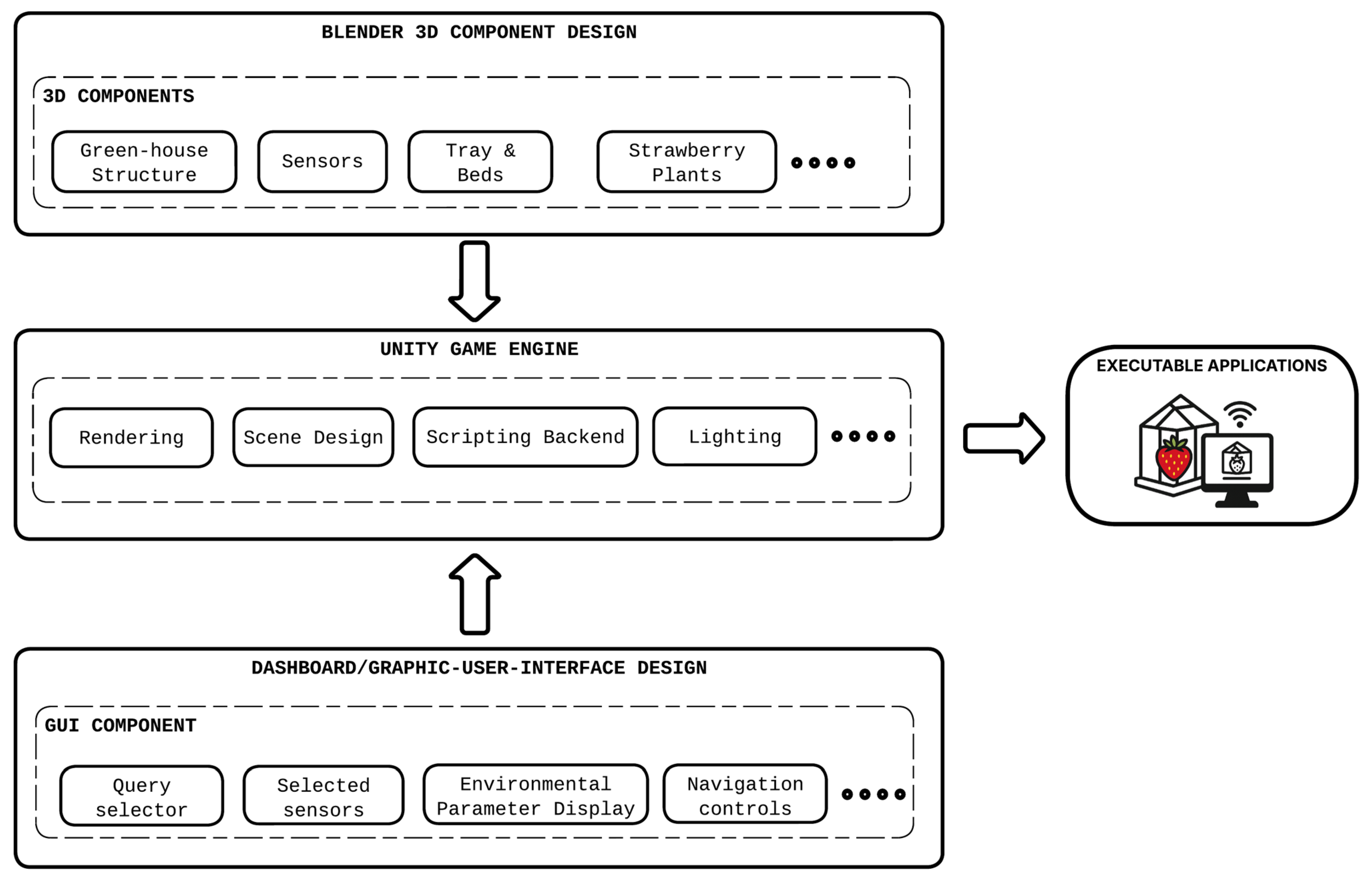
Figure 6 summarizes the development workflow adopted for the strawberry-greenhouse digital twin. All geometry listed in

Table 2. A description of GUI components used in the virtual environment, highlighting features for temporal query selection and navigation within the 3D space.

GUI Components	Description
Query Selection	Users can select specific parameters for their analysis, focusing on choosing the month of interest. This temporal selection is crucial for analyzing seasonal variations in greenhouse conditions.
Navigation Controls	Users can navigate through the 3D environment using controls integrated into the GUI. DT users can also navigate. The temperature and relative humidity are visualized by selecting the sensors, enabling the Monitoring of the spatial variation in the greenhouse microclimate.

was first constructed in Blender using field measurements as constraints. Every mesh shared a common origin and naming convention, ensuring that the exported FBX bundle preserved spatial fidelity when imported into Unity. Inside Unity, these assets were converted to prefabs and organized in a master scene. A lightweight scripting layer then linked each sensor prefab to a REST endpoint that supplies temperature and relative humidity streams at five-second intervals. The same data feed populates the dashboard widgets documented in

Table 3. Key 3D components of the virtual Greenhouse and their physical correspondences.

3D Components	Description
Greenhouse Structure	A virtual representation of the Greenhouse, modeled to scale based on the physical structure.
Sensors	Virtual representations of the 56 sensors placed throughout the Greenhouse accurately reflect their positions in physical space.
Strawberry Plants	3D Models of strawberry plants provide visual cues about plant health and development.
Plant Beds	A virtual representation of the five plant beds, modeled to the specifications of 15 m in length, 0.26 m in width, and placed at a height of 1.1 m.
Strawberry Pots	Individual pots for each strawberry plant.
Ground Sand	A textured representation of the greenhouse floor, adding to the visual realism of the environment.

, which were implemented with Unity UI Toolkit and docked alongside the three-dimensional viewport. Finally, the scene, scripts, and interface were compiled into an Executable application that mirrors greenhouse conditions in real-time, while retaining the structural and navigational context established during the Blender phase.

4. Results

4.1. Selected Sensor Locations

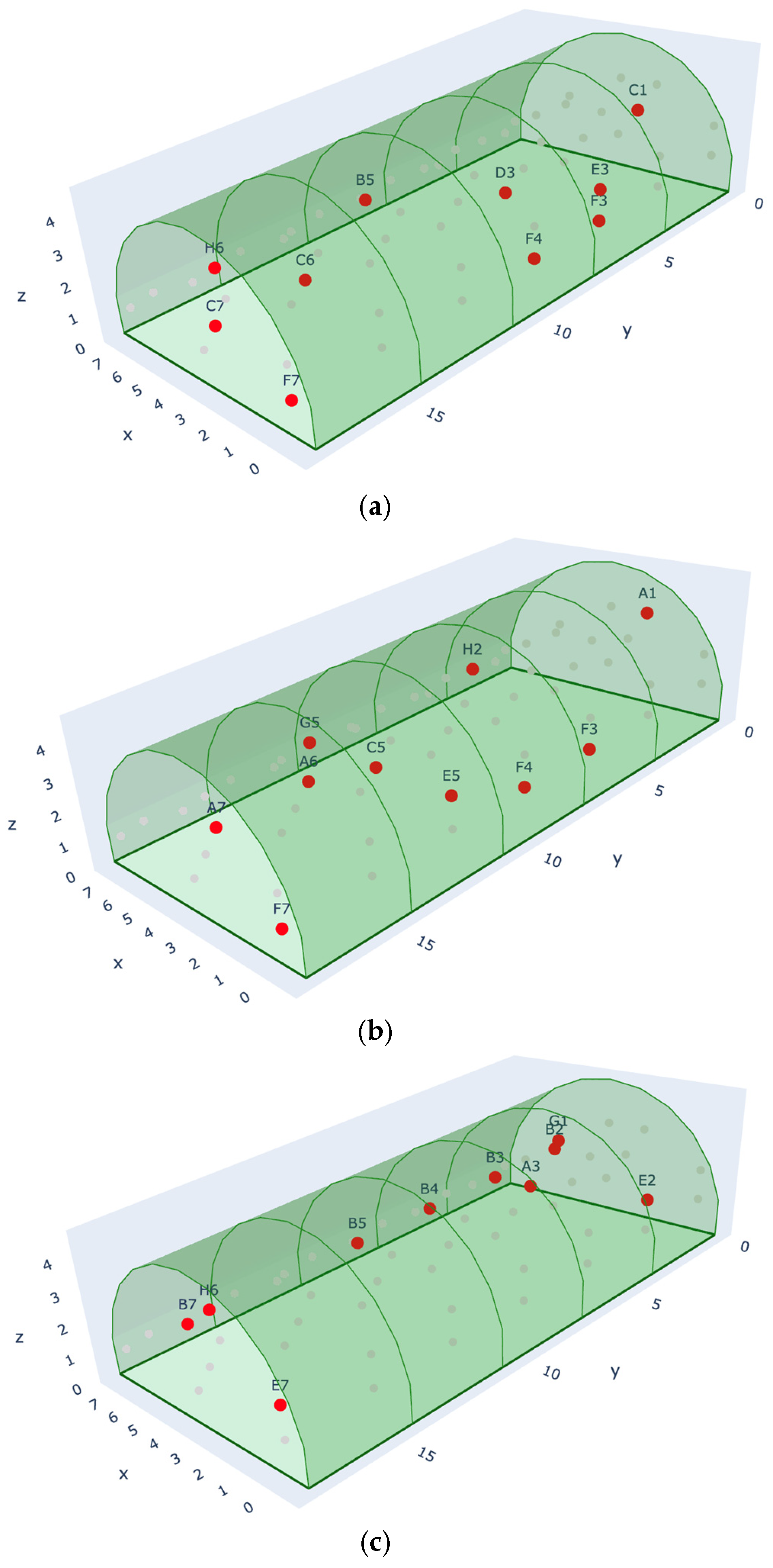
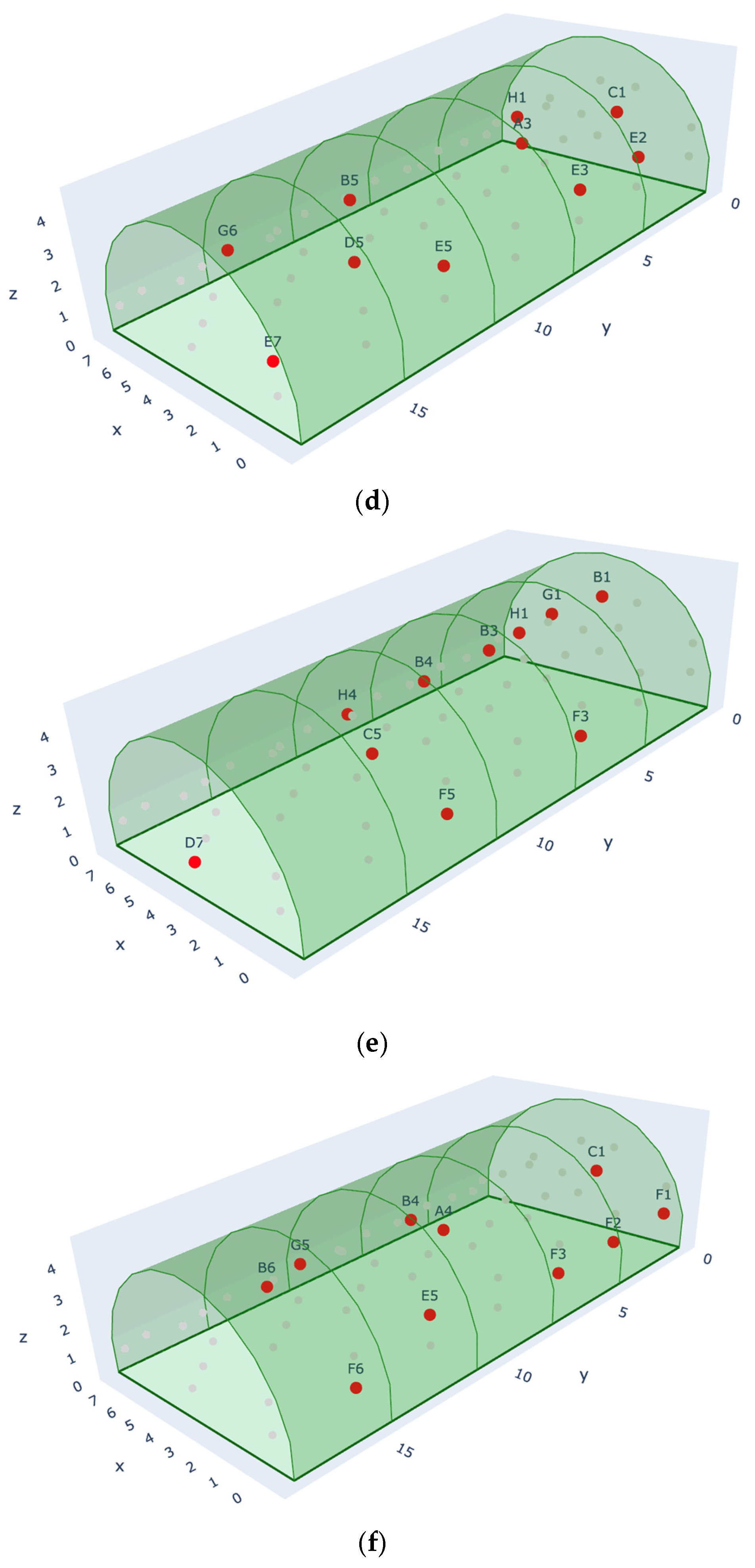
The spatial distributions of the ten highest-ranked sensors for each psychrometric variable of temperature, relative humidity (RH), Enthalpy, humidity ratio, specific volume, and dew point are visualized in Figure 7a–f. These distributions tell variable-specific spatial sensitivities, with minimal overlap among sensor locations. For instance, temperature maxima during the winter months are consistently localized near the northeast roof arch (Figure 7a), indicating thermal stratification patterns that are likely influenced by greenhouse geometry and airflow dynamics. In contrast, the top-performing RH sensors were consistently located along the southwestern sidewall (Figure 7b), suggesting that moisture gradients follow distinct pathways that are decoupled from thermal profiles. The remaining variables, enthalpy (Figure 7c), humidity ratio (Figure 7d), specific volume (Figure 7e), and dew point (Figure 7f), exhibited yet other optimal spatial configurations, collectively reinforcing the non-uniform and variable-dependent nature of microclimatic heterogeneity within the controlled environment(see

Table 4. Seasonal Top 10 Sensor Rankings for each variable Monitoring in the Greenhouse [23].

Season	Parameter	Rank 1	Rank 2	Rank 3	Rank 4	Rank 5	Rank 6	Rank 7	Rank 8	Rank 9	Rank 10
Winter	RH (%)	F7	A6	F3	E5	G5	A7	C5	H2	A1	F4
	SV (m3/kg)	B3	F5	H4	F3	D7	B1	H1	G1	B4	C5
	Td (°C)	C1	A4	F6	B4	B6	G5	E5	F3	F2	F1
	Temp (°C)	C1	C7	E3	H6	F3	F7	D3	C6	F4	B5
	W (kg/kg)	G6	E2	E7	D5	H1	B5	E3	E5	A3	C1
	h (kJ/kg)	E2	A3	B2	B3	G1	B4	B7	E7	H6	B5
Spring	RH (%)	F4	B3	C4	D4	D5	D7	F6	F7	F5	E4
	SV (m3/kg)	E2	G4	D2	E4	E5	B4	H6	G1	D4	D6
	Td (°C)	E4	F5	B1	A7	D1	E2	C5	F6	C2	D7
	Temp (°C)	G1	A2	B6	D2	H2	E7	G2	B4	G4	E5
	W (kg/kg)	C4	E4	H1	H6	G6	C1	G1	F3	D7	A2
	h (kJ/kg)	F1	D3	F4	D1	D6	E1	C6	A4	E2	C1
Summer	RH (%)	G5	A7	D3	G4	G5	H2	E4	D2	D6	C6
	SV (m3/kg)	A4	A6	E6	A3	G4	H7	D2	D7	F6	G2
	Td (°C)	E6	G6	A4	G4	F7	C6	A6	D1	B2	G1
	Temp (°C)	H1	H6	H3	G7	A3	D3	F6	C4	G4	G2
	W (kg/kg)	H4	E3	E2	C1	G7	G1	B1	D6	H1	G3
	h (kJ/kg)	D4	A2	E4	B3	C3	F5	A6	A5	E6	D5
Autumn	RH (%)	C5	A2	H3	H6	A5	F3	G5	G7	H2	A1
	SV (m3/kg)	C1	E4	C6	E3	A5	F1	A6	A2	C2	D1
	Td (°C)	A5	F2	E3	B2	E4	C3	E7	H6	D7	B3
	Temp (°C)	C4	C6	D4	F3	H5	B7	F2	G6	E6	G5
	W (kg/kg)	D4	G2	F1	H4	B2	A5	D2	D6	F3	A4
	h (kJ/kg)	E1	D4	H7	A5	A2	E6	D5	B2	D1	D7

).

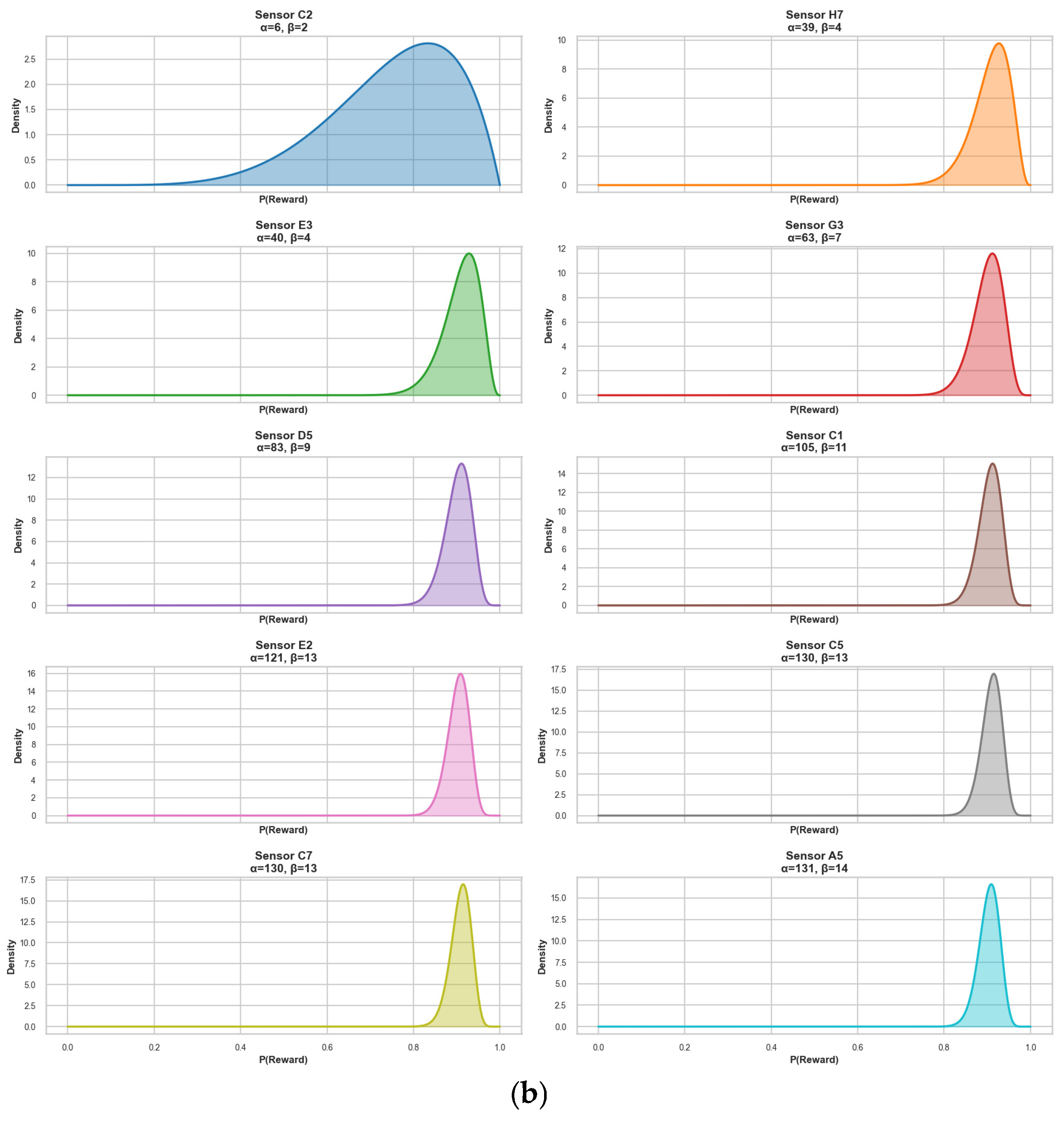
Bayesian inference applied to April’s temperature dataset further substantiates the sensor ranking outcomes. The Beta posterior distributions corresponding to the top-ranked temperature sensors, G1, A2, and B6, exhibit sharply peaked unimodal profiles (Figure 8a), characterized by α and fβ. These statistical properties indicate a high likelihood of accurate mean-crossing detection and tight confidence intervals. In contrast, lower-ranked sensors display flatter posteriors with extended tails (Figure 8b), reflecting increased uncertainty and reduced reliability in capturing representative thermal conditions. The divergence between the optimal locations of the temperature and RH sensors highlights a critical constraint in dual-channel sensing architectures. Specifically, co-locating temperature and RH transducers in a single physical package would inevitably place one parameter in a suboptimal sensing zone, thereby diminishing measurement fidelity. This observation strongly supports the deployment of variable-specific sensor arrays, optimized for spatial performance on a per-parameter basis.

Cross-seasonal analysis reveals that the spatial centroids of the top-ranked sensor clusters for each variable undergo systematic migration, up to 4 m, between winter and summer months. This seasonal drift highlights the dynamic nature of environmental gradients in semi-controlled protected environmental systems, supporting the implementation of temporally adaptive sensing configurations. These findings suggest that approximately 70% of the full 56-node sensor network provides redundant information under current operating conditions. Notably, most high-performing sensors reside at peripheral rather than central locations, challenging conventional assumptions of uniform central coverage. These results provide empirical justification for a streamlined, single-parameter sensor deployment strategy that is both spatially and temporally optimized. Such a strategy can significantly reduce hardware operation costs while maintaining, or even improving, the resolution and fidelity of environmental monitoring in digitally twinned agricultural systems.

Figure 9a–c shows that the chosen subset of sensors did not perform the same way for temperature and relative humidity. For temperature, the MAE and RMSE values stayed low across the seasons, meaning a smaller set of sensors was enough to follow the overall trend in the Greenhouse. For relative humidity, the errors were much higher, showing that the subset missed important variations and could not fully represent the greenhouse conditions. The z-index results confirm this: while temperature readings stayed consistent with little overlap, relative humidity sensors often carried redundant information, with several sensors measuring almost the same thing. This means that, in practice, temperature is easier to track with fewer sensors, but relative humidity requires either more sensors or better placement to avoid gaps and repetition.

4.2. Unity Greenhouse Environment

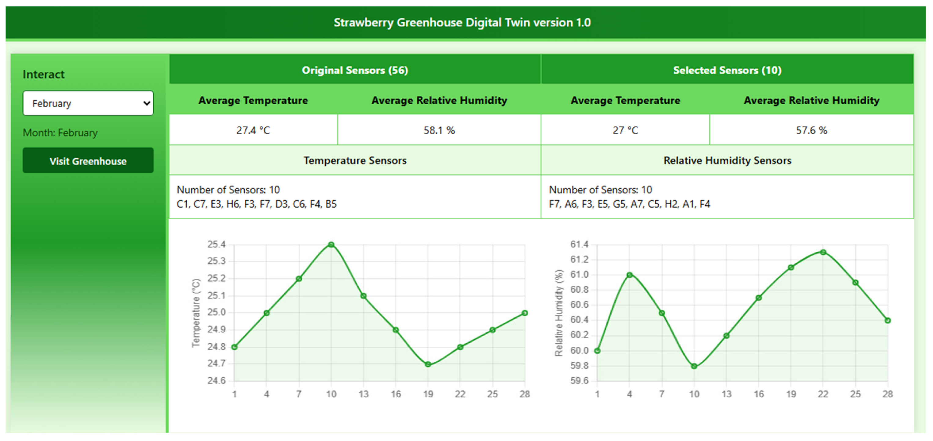
Figure 10 presents a graphical representation of the Strawberry Greenhouse Digital Twin interface, captured after the user selects “February” from the interactive dropdown menu. The graphical user interface (GUI) simultaneously displays data from the complete sensor network (n = 56) and a computationally derived subset (n = 10), determined through sensor optimization algorithms. Sensor node identifiers are enumerated beneath each corresponding sparkline, providing compact temporal visualizations of microclimatic data. Summary statistics are displayed for both configurations, revealing minimal divergence in environmental metrics. The complete set records a mean temperature of 27.4 °C and a relative humidity of 58.1%, while the reduced set registers corresponding values of 27.0 °C and 57.6%, respectively. This high degree of numerical concordance quantitatively demonstrates the preservation of informational integrity despite an 82% reduction in hardware deployment. Such results underscore the effectiveness of the sensor selection algorithm in maintaining system observability with significantly lower sensing density.

An interface-anchored “Visit Greenhouse” button initiates a transition to a Unity-based immersive environment, enabling users to enter a fully rendered, three-dimensional (3D) virtual model of the Greenhouse. Within this environment, all structural and environmental sensing components, including strawberry beds, metallic arch supports, and sensor nodes, are spatially reconstructed at a 1:1 scale. Sensor status is denoted through visual encoding: deactivated nodes appear as translucent, desaturated spheres, while the algorithmically prioritized subset is rendered as opaque, high-saturation red spheres. These ten optimized nodes are spatially distributed across key vertical zones, roof, sidewalls, and canopy, demonstrating algorithmic spatial coverage and avoiding spatial redundancy or clustering (see Figure 11).

The 2D dashboard and the immersive 3D interface deliver a hybrid analytical–experiential platform, integrating statistical validation with spatial cognition. The visual coherence of this digital twin architecture facilitates user comprehension while minimizing cognitive load, enabling efficient interpretation and informed decision-making for greenhouse climate monitoring.

4.3. Data Transfer Assessment

The data-management layer of the strawberry-greenhouse digital twin performs two complementary duties: retrieving live measurements to ensure that the virtual model accurately mirrors the physical environment and persisting those measurements for downstream analytics. Live readings are exposed through an API, providing client services with a uniform interface. Meanwhile, the same streams are published using MQTT to minimize message overhead and decouple publishers from subscribers. Figure 12 plots request-processing latency against the number of sensor data points returned in a single call; latency rises gradually below one-hundred-thousand points, then accelerates once the payload exceeds roughly three-hundred thousand, eventually reaching just over fifty seconds at 1.7 million points. This nonlinear growth implies that very dense sampling or overly large query batches can erode the real-time responsiveness expected of the digital twin. Responsiveness, therefore, hinges on limiting unnecessary traffic, which can be achieved by optimizing sensor placements so that sensing instruments are installed only where they add unique information and by segmenting historical queries into smaller windows, applying server-side pagination to keep each call below the observed inflection point [38]. Without such safeguards, rising payloads will lengthen feedback cycles and increase the platform’s downtime, undermining the reliability of both the virtual model and any decision-support services built upon it.

5. Future Works and Discussions

Future investigations would extend the data-driven adaptable-sensor architecture presented here by embedding crop-growth simulation within the digital twin itself [39]. Coupling high-resolution microclimate readings with mechanistic or data-driven growth models can provide real-time forecasts of phenological milestones, biomass accumulation, and eventual yield. This fusion will explain how localized temperature, relative humidity, and luminance profiles, captured by optimally placed sensors, influence productivity, thereby facilitating more precise irrigation, nutrient dosing, and harvest orchestration. A further priority involves enriching the twin with high-fidelity three-dimensional reconstructions of both the greenhouse envelope and the crop canopy [40]. Periodic 3D imaging supplies geometric granularity that supports automated growth-rate quantification, occlusion illumination or spraying schemes, and rigorous validation of growth-model projections [41]. Complementary simulations of greenhouse ventilation, attained with computational fluid dynamics, would define spatiotemporal gradients of temperature, relative humidity, and carbon dioxide concentration. Integrating these airflow models with live sensor feedback enables proactive climate regulation, dynamic vent scheduling, and fan-speed modulation, thereby balancing crop needs with energy stewardship. Subsequent inquiry should also benchmark alternative sensor-deployment heuristics beyond the Thompson-sampling protocol employed here. Candidate strategies include K-means++ clustering, information-theoretic configurations, and reinforcement-learning bandits responsive to seasonal variability. Equally important is a cost assessment of the impact of reducing sensor locations from 56 to 10, to ensure that gains in computational efficiency and reduced redundancy do not come at the expense of critical spatial coverage. Future research would fine-tune the digital twin framework by incorporating additional environmental parameters, such as light intensity, soil moisture, and CO₂ levels, to create a more holistic monitoring system. Expanding the predictive capabilities of the digital twin through advanced machine learning models will enable the anticipation of climate control adjustments and crop growth patterns. Furthermore, exploring the scalability of this framework across diverse greenhouse systems and its integration with IoT networks can unlock broader applications, including resource conservation.

6. Conclusions

The study demonstrates how a Unity-based digital twin, coupled with a Thompson sampling reinforcement learning routine, can streamline environmental monitoring in a greenhouse. Over four seasons of archived data, the algorithm repeatedly selected ten-sensor subset whose mean temperature and relative humidity remained within 0.4 °C and 0.5% RH of the 56-node network, demonstrating strong representational fidelity while reducing hardware needs. More than 70% of deployed sensors contributed little unique information, and temperature-versus-relative humidity optima rarely coincided, highlighting both the redundancy of the existing layout and the limitations of two-in-one sensors. Beyond spatial efficiency, the data-transfer audit showed that request latency increases sharply once a payload exceeds approximately 300,000 records, surpassing 50s at 1.7 million points. Keeping queries below this through pagination and by avoiding redundant measurements protects the near-real-time performance expected of the twin. The work focuses solely on temperature and relative humidity derivable variables, leaving other agronomic variables untested. The reinforcement-learning was trained offline, so its behavior under live retraining remains unverified. Additionally, the results are limited by the use of a single greenhouse, which restricts generalizability. Future research would extend the framework with online learning, additional climate and crop-growth parameters, CFD-based airflow models, and comparative placement heuristics such as clustering.

References

1. Maraveas, C.; Bartzanas, T. Application of Internet of Things (IoT) for Optimized Greenhouse Environments. Agriengineering 2021, 3, 954–970. [Google Scholar] [CrossRef]
2. Maraveas, C.; Karavas, C.-S.; Loukatos, D.; Bartzanas, T.; Arvanitis, K.G.; Symeonaki, E. Agricultural Greenhouses: Resource Management Technologies and Perspectives for Zero Greenhouse Gas Emissions. Agriculture 2023, 13, 1464. [Google Scholar] [CrossRef]
3. Slob, N.; Hurst, W.; van de Zedde, R.; Tekinerdogan, B. Virtual reality-based digital twins for greenhouses: A focus on human interaction. Comput. Electron. Agric. 2023, 208, 107815. [Google Scholar] [CrossRef]
4. Qi, Q.; Tao, F.; Hu, T.; Anwer, N.; Liu, A.; Wei, Y.; Wang, L.; Nee, A.Y.C. Enabling technologies and tools for digital twin. J. Manuf. Syst. 2021, 58, 3–21. [Google Scholar] [CrossRef]
5. Iliuţă, M.-E.; Moisescu, M.-A.; Pop, E.; Ionita, A.-D.; Caramihai, S.-I.; Mitulescu, T.-C. Digital Twin—A Review of the Evolution from Concept to Technology and Its Analytical Perspectives on Applications in Various Fields. Appl. Sci. 2024, 14, 5454. [Google Scholar] [CrossRef]
6. Wright, L.; Davidson, S. How to tell the difference between a model and a digital twin. Adv. Model. Simul. Eng. Sci. 2020, 7, 13. [Google Scholar] [CrossRef]
7. Jones, D.; Snider, C.; Nassehi, A.; Yon, J.; Hicks, B. Characterising the Digital Twin: A systematic literature review. CIRP J. Manuf. Sci. Technol. 2020, 29, 36–52. [Google Scholar] [CrossRef]
8. Tagarakis, A.C.; Benos, L.; Kyriakarakos, G.; Pearson, S.; Sørensen, C.G.; Bochtis, D. Digital Twins in Agriculture and Forestry: A Review. Sensors 2024, 24, 3117. [Google Scholar] [CrossRef]
9. Escribà-Gelonch, M.; Liang, S.; van Schalkwyk, P.; Fisk, I.; Long, N.V.D.; Hessel, V. Digital Twins in Agriculture: Orchestration and Applications. J. Agric. Food Chem. 2024, 72, 10737–10752. [Google Scholar] [CrossRef]
10. Peladarinos, N.; Piromalis, D.; Cheimaras, V.; Tserepas, E.; Munteanu, R.A.; Papageorgas, P. Enhancing Smart Agriculture by Implementing Digital Twins: A Comprehensive Review. Sensors 2023, 23, 7128. [Google Scholar] [CrossRef]
11. Pylianidis, C.; Osinga, S.; Athanasiadis, I.N. Introducing digital twins to agriculture. Comput. Electron. Agric. 2021, 184, 105942. [Google Scholar] [CrossRef]
12. Lema-Rumińska, J.; Kulus, D.; Tymoszuk, A.; Miler, N.; Wozny, A.; Wenda-Piesik, A. Physiological, Biochemical, and Biometrical Response of Cultivated Strawberry and Wild Strawberry in Greenhouse Gutter Cultivation in the Autumn-Winter Season in Poland—Preliminary Study. Agronomy 2021, 11, 1633. [Google Scholar] [CrossRef]
13. de Miranda, F.R.; da Silva, V.B.; Santos, F.S.R.D.; Rossetti, A.G.; da Silva, C.D.F.B. Production of Strawberry Cultivars in Closed Hydroponic Systems and Coconut Fibre Substrate. Rev. Ciência Agronômica 2014, 45, 833–841. [Google Scholar] [CrossRef]
14. DeLay, N.D.; Thompson, N.M.; Mintert, J.R. Precision Agriculture Technology Adoption and Technical Efficiency. J. Agric. Econ. 2021, 73, 195–219. [Google Scholar] [CrossRef]
15. Lian, Y.; Wang, A.; Peng, S.; Jia, J.; Zong, L.; Yang, X.; Li, J.; Zheng, R.; Yang, S.; Liao, J.; et al. Optimization of Sensors Data Transmission Paths for Pest Monitoring Based on Intelligent Algorithms. Biosensors 2022, 12, 948. [Google Scholar] [CrossRef]
16. Uyeh, D.D.; Iyiola, O.; Mallipeddi, R.; Asem-Hiablie, S.; Amaizu, M.; Ha, Y.; Park, T. Grid Search for Lowest Root Mean Squared Error in Predicting Optimal Sensor Location in Protected Cultivation Systems. Front. Plant Sci. 2022, 13, 920284. [Google Scholar] [CrossRef]
17. Sánchez, D.C.; Sanchez-Londono, A.; Barbieri, G. A Digital Twin Architecture to Optimize Productivity within Controlled Environment Agriculture. Appl. Sci. 2021, 11, 8875. [Google Scholar] [CrossRef]
18. Purcell, W.; Neubauer, T.; Mallinger, K. Digital Twins in agriculture: Challenges and opportunities for environmental sustainability. Curr. Opin. Env. Sustain. 2023, 61, 102152. [Google Scholar] [CrossRef]
19. Ajani, O.S.; Aboyeji, E.; Mallipeddi, R.; Uyeh, D.D.; Ha, Y.; Park, T. A genetic programming-based optimal sensor placement for greenhouse monitoring and control. Front. Plant Sci. 2023, 14, 1152036. [Google Scholar] [CrossRef]
20. Lee, S.Y.; Lee, I.B.; Yeo, U.H.; Kim, R.W.; Kim, J.G. Optimal sensor placement for monitoring and controlling greenhouse internal environments. Biosyst. Eng. 2019, 188, 190–206. [Google Scholar] [CrossRef]
21. Ferentinos, K.P.; Katsoulas, N.; Tzounis, A.; Bartzanas, T.; Kittas, C. Wireless sensor networks for greenhouse climate and plant condition assessment. Biosyst. Eng. 2017, 153, 70–81. [Google Scholar] [CrossRef]
22. Uyeh, D.; Akinsoji, A.; Asem-Hiablie, S.; Bassey, B.; Osinuga, A.; Mallipeddi, R.; Amaizu, M.; Ha, Y.; Park, T. An online machine learning-based sensors clustering system for efficient and cost-effective environmental monitoring in controlled environment agriculture. Comput. Electron. Agric. 2022, 199. [Google Scholar] [CrossRef]
23. Uyeh, D.; Bassey, B.; Mallipeddi, R.; Asem-Hiablie, S.; Amaizu, M.; Seungmin, W.; Ha, Y.; Park, T. A reinforcement learning approach for optimal placement of sensors in protected cultivation systems. IEEE Access 2021, 9, 100781–100800. [Google Scholar] [CrossRef]
24. Lang, Y.; Zhang, Y.; Sun, T.; Chai, X.; Zhang, N. Digital twin-driven system for efficient tomato harvesting in greenhouses. Comput. Electron. Agric. 2025, 236, 110451. [Google Scholar] [CrossRef]
25. Defraeye, T.; Shrivastava, C.; Berry, T.; Verboven, P.; Onwude, D.; Schudel, S.; Bühlmann, A.; Cronje, P.; Rossi, R.M. Digital twins are coming: Will we need them in supply chains of fresh horticultural produce? Trends Food Sci. Technol. 2021, 109, 245–258. [Google Scholar] [CrossRef]
26. Ghandar, A.; Ahmed, A.; Zulfiqar, S.; Hua, Z.; Hanai, M.; Theodoropoulos, G. A Decision Support System for Urban Agriculture Using Digital Twin: A Case Study With Aquaponics. IEEE Access 2021, 9, 35691–35708. [Google Scholar] [CrossRef]
27. Howard, D.A.; Ma, Z.; Veje, C.; Clausen, A.; Aaslyng, J.M.; Jørgensen, B.N. Greenhouse industry 4.0-digital twin technology for commercial greenhouses. Energy Inform. 2021, 4, 37. [Google Scholar] [CrossRef]
28. Spyrou, O.; Hurst, W.; Verdouw, C. Virtual Reality-Based Digital Twins: A Case Study on Pharmaceutical Cannabis. Big Data Cogn. Comput. 2023, 7, 95. [Google Scholar] [CrossRef]
29. Ko, T.-H.; Lee, H.-M.; Noh, D.-H.; JuHwan, C.; Byun, S.-W. Design and Implementation of a Digital Twin Platform in Vertical Farming Systems. In Proceedings of the 2022 Thirteenth International Conference on Ubiquitous and Future Networks (ICUFN), Barcelona, Spain, 5–8 July 2022; pp. 366–368. [Google Scholar] [CrossRef]
30. Clements, P.; Garlan, D.; Little, R.; Nord, R.; Stafford, J. Documenting software architectures: Views and beyond. In Proceedings of the 25th International Conference on Software Engineering, Portland, OR, USA, 3–10 May 2003; pp. 740–741. [Google Scholar] [CrossRef]
31. Niu, Z. Research and Implementation of Internet of Things Communication System Based on MQTT Protocol. J. Phys. Conf. Ser. 2021, 2023, 12019. [Google Scholar] [CrossRef]
32. Howard, D.A.; Ma, Z.; Aaslyng, J.M.; Jørgensen, B.N. Data Architecture for Digital Twin of Commercial Greenhouse Production. In Proceedings of the 2020 RIVF International Conference on Computing and Communication Technologies (RIVF), Ho Chi Minh City, Vietnam, 14–15 October 2020; pp. 1–7. [Google Scholar] [CrossRef]
33. Niranjanamurthy, M.; Archana, U.L.; Niveditha, K.T.; Jafar, S.A.; Shravan, N.S. The research study on DynamoDB—NoSQL database service. Int. J. Comput. Sci. Mob. Comput. 2014, 3, 268–279. [Google Scholar]
34. Grant, J.; Boukouvalas, A.; Griffiths, R.-R.; Leslie, D.; Vakili, S.; De Cote, E.M. Adaptive Sensor Placement for Continuous Spaces. In Proceedings of the ICML 2019: 36th International Conference on Machine Learning, Long Beach, CA, USA, 10–15 June 2019; Chaudhuri, K., Salakhutdinov, R., Eds.; ICML, 2019. Volume 97. Available online: https://proceedings.mlr.press/v97/grant19a.html (accessed on 14 September 2025).
35. Wang, C.; Huang, V.; Chen, G.; Ma, H.; Chen, B.; Schmidt, J. Learning to Optimise Climate Sensor Placement Using a Transformer. Available online: https://api.semanticscholar.org/CorpusID:264306116 (accessed on 14 September 2025).
36. Bua, C.; Borgianni, L.; Adami, D.; Giordano, S. Reinforcement Learning-Driven Digital Twin for Zero-Delay Communication in Smart Greenhouse Robotics. Agriculture 2025, 15, 1290. [Google Scholar] [CrossRef]
37. Arnesano, M.; Revel, G.M.; Seri, F. A tool for the optimal sensor placement to optimize temperature monitoring in large sports spaces. Autom. Constr. 2016, 68, 223–234. [Google Scholar] [CrossRef]
38. Shukla, S.; Hassan, M.F.; Tran, D.C.; Akbar, R.; Paputungan, I.V.; Khan, M.K. Improving latency in Internet-of-Things and cloud computing for real-time data transmission: A systematic literature review (SLR). Clust. Comput. 2023, 26, 2657–2680. [Google Scholar] [CrossRef]
39. Drees, L.; Demie, D.T.; Paul, M.R.; Leonhardt, J.; Seidel, S.J.; Döring, T.F.; Roscher, R. Data-driven crop growth simulation on time-varying generated images using multi-conditional generative adversarial networks. Plant Methods 2024, 20, 1. [Google Scholar] [CrossRef]
40. Li, W.; Zhu, D.; Wang, Q. A single view leaf reconstruction method based on the fusion of ResNet and differentiable render in plantgrowthdigitaltwinsystem. Comput. Electron. Agric. 2022, 193, 106712. [Google Scholar] [CrossRef]
41. Jiqing, C.; Jiahua, W.; Zhikui, W.; Hu, Q.; Ganwei, C.; Chengzhi, T.; Chaoyang, Z. Detecting ripe fruits under natural occlusion and illumination conditions. Comput. Electron. Agric. 2021, 190, 106450. [Google Scholar] [CrossRef]
Figure 1. Interconnection of Digital Twin Greenhouse System Components.
Agriengineering 07 00315 g001
Figure 2. An interior photograph (top) and a 3D diagram (bottom) together show the positions of 56 temperature–relative humidity sensors (A1–H7) within the Greenhouse [23].
Agriengineering 07 00315 g002
Figure 3. (a) Spatial gradient of mean air temperature in the Greenhouse across winter, spring, summer, and autumn. (b) Spatial distribution of mean relative humidity levels in the Greenhouse across winter, spring, summer, and autumn. (c) Spatial distribution of average specific volume (m3/kg) of moist air in the Greenhouse across winter, spring, summer, and autumn. (d) Visualization of spatial differences in mean Enthalpy (kJ/kg) in the Greenhouse across winter, spring, summer, and autumn. (e) Spatial gradient of mean relative humidity ratio (kg water/kg dry air) in the Greenhouse across winter, spring, summer, and autumn. (f) The surface plot shows spatial variation in average dew point temperature across winter, spring, summer, and autumn.
Agriengineering 07 00315 g003aAgriengineering 07 00315 g003b
Figure 4. Data Flow sequence for the digital twin.
Agriengineering 07 00315 g004
Figure 5. Flow sequence from initialization to posterior update within the greenhouse digital twin.
Agriengineering 07 00315 g005
Figure 6. Digital twin architecture integrating 3D modeling, game engine simulation, and GUI for greenhouse monitoring applications.
Agriengineering 07 00315 g006
Figure 7. (a) Top 10 Temperature Sensors in February within the Greenhouse. (b) Top 10 Relative Humidity Sensors in February within the Greenhouse. (c) Top 10 Enthalpy Sensors in February within the Greenhouse. (d) Top-10 Humidity Ratio Sensors in February within the Greenhouse. (e) Top 10 Specific Volume Sensors in February within the Greenhouse. (f) Top 10 Dewpoint Sensors in February within the Greenhouse.
Agriengineering 07 00315 g007aAgriengineering 07 00315 g007b
Figure 8. (a) Posterior distributions of sensor selection probabilities (P(Reward)) for the top 10 sensors selected for temperature monitoring in April using Thompson Sampling. (b) Posterior distributions of sensor selection probabilities (P(Reward)) for the bottom 10 sensors selected for temperature monitoring in April using Thompson Sampling.
Agriengineering 07 00315 g008aAgriengineering 07 00315 g008b
Figure 9. (a) MAE across seasons for Temperature and Relative Humidity. (b) RMSE across seasons for Temperature and Relative Humidity. (c) Z-index across seasons for Temperature and Relative Humidity.
Agriengineering 07 00315 g009
Figure 10. Virtual Environment of the Strawberry Greenhouse Digital Twin System. (a) Temperature–Relative Humidity sensor, (b) strawberry plants, (c) External view of the greenhouse structure, (d) view of the internal greenhouse structure.
Agriengineering 07 00315 g010
Figure 11. A Graphical User Interface (GUI) of the Strawberry Greenhouse Digital Twin System, visualizing sensor readings from February.
Agriengineering 07 00315 g011
Figure 12. Request latency versus sensor data points, illustrating a nonlinear rise in processing time as the payload grows.
Agriengineering 07 00315 g012