ChickenSense: A Low-Cost Deep Learning-Based Solution for Poultry Feed Consumption Monitoring Using Sound Technology

Abstract

This research proposes a low-cost system consisting of a hardware setup and a deep learning-based model to estimate broiler chickens’ feed intake, utilizing audio signals captured by piezoelectric sensors. The signals were recorded 24/7 for 19 consecutive days. A subset of the raw data was chosen, and events were labeled in two classes, feed-pecking and non-pecking (including singing, anomaly, and silence samples). Next, the labeled data were preprocessed through a noise removal algorithm and a band-pass filter. Then, the spectrogram and the signal envelope were extracted from each signal and fed as inputs to a VGG-16-based convolutional neural network (CNN) with two branches for 1D and 2D feature extraction followed by a binary classification head to classify feed-pecking and non-pecking events. The model achieved 92% accuracy in feed-pecking vs. non-pecking events classification with an f1-score of 91%. Finally, the entire raw dataset was processed utilizing the developed model, and the resulting feed intake estimation was compared with the ground truth data from scale measures. The estimated feed consumption showed an 8 ± 7% mean percent error on daily feed intake estimation with a 71% R2 score and 85% Pearson product moment correlation coefficient (PPMCC) on hourly intake estimation. The results demonstrate that the proposed system estimates broiler feed intake at each feeder and has the potential to be implemented in commercial farms.

1. Introduction

Broilers’ feed intake and feeding behaviors are important animal-based measurements that may indicate their welfare conditions. These data may provide insightful information to help achieve a better feed conversion ratio (FCR) and improved health and welfare status [1]. While current sensing systems in commercial farms, feed bin scales, can measure accurately the daily feed delivered to each broiler house, they do not provide information such as when and where the broilers eat and how much time the broilers spend eating. That information may be used to identify potential equipment-related and environmental issues, such as clogged feeders and wet litter in certain areas, and help us study the impact of various farm settings on broilers welfare and health conditions.

Due to the recent advance in machine learning and computer vision, camera systems have been widely investigated by researchers in poultry farming for studying welfare-related behaviors (e.g., feeding, drinking, stretching, pruning, and dust bathing), health condition assessment (e.g., gait score and plumage condition), and weight estimation [2,3,4]. In a few recent studies, computer vision techniques were used to segment the feeding and drinking area, detect chickens, and calculate the estimated number of broiler chickens surrounding the feeder or drinker at each frame [5,6]. Although these methods achieved reasonable performance in capturing the feeding behavior trend, it was challenging for the models to distinguish between feeding behaviors and non-feeding behaviors when the broilers were at the feeders, for example, broilers standing idle at the feeders versus broilers eating; as a result, the feeding event determined by the previous studies was usually defined as the presence of chickens in the feeding area. In addition to this issue, computer vision-based methods often struggle with the problem of occluded chickens [7], poor lighting conditions, and low resolution, which may lead to decreases in the overall accuracy of the estimations. Besides the challenges in applying computer vision systems in poultry monitoring, most computer vision-based systems require high-performance computers equipped with graphical processing units (GPUs) to process data in real-time, resulting in a drastic increase in expenses to deploy the models on a commercial scale.

Besides cameras systems, researchers have also developed and evaluated other types of sensors. Several groups of researchers applied time-series data of feed weight collected from scales to investigate broilers’ feeding behaviors, such as the number of meals per day, feeding pattern, meal duration, growth rate, and feed conversion ratio [8,9,10]. Despite high-precision results, using scales at each feeder pan is more suitable for laboratory-scale studies than farm-scale studies due to the high costs to install many weight scales and the difficulty in measuring the weight of each feeder pan independently. Another important issue with scale-based systems is the requirement to calibrate the scales intermittently, which is a labor-intensive process.

Moreover, several studies using sound-based systems have shown the potential of this technique for feed intake measurements. Aydin et al. developed a microphone-based system to measure the feed-pecking at each feeder [11]. They studied the correlation between the number of feed-pecking events and the actual feed consumption using a sound classification method and achieved an accuracy of 90% in feed intake estimation. The study was performed in an experimental setup with one chicken per pen. In a later study with ten chickens in pen, the group achieved an accuracy of 86% [12]. Another group also investigated the use of microphones for broiler feeding behavior detection. Huang et al. extracted the short-time energy (STE) and short-time zero crossing rates (STZ) as the main features from audio signals to classify feeding and non-feeding vocalization events based on a recurrent neural network [13]. The proposed model achieved 96% accuracy, demonstrating the usefulness of acoustic features as a non-invasive approach to studying poultry behaviors.

Although the previous audio-based methods achieved encouraging results, several challenges still need to be addressed in order for this technology to be practical for field implementation. First, the cost of the system must be very cheap for commercial poultry farms, which usually have thousands of feeder pans. Even with a small spatial sampling rate, e.g., 5–10%, there are still hundreds of feeder pans to be monitored. Given the thin profit margin in the poultry industry, lowering the cost of such a system is one of the priorities. Second, the information of feed-pecking from the broilers needs to be combined with other relevant information to provide meaningful insights into the birds or farm conditions for the farmers. Therefore, such an audio-based sensing system is better justified when combined with other sensors, e.g., a camera system, which will likely require system integration and algorithm development and optimization. Third, the system must be easily installed and implemented in commercial farms where various limitations need to be considered. While we do not attempt to resolve all of the challenges at once, our goal is to evaluate a sensor that offers us the potential to mitigate those challenges.

Recently, one of the exciting areas in machine learning is named TinyML, which refers to applying machine learning models on an ultra-low-power microcontroller that consumes less than 1 milliWatt of power [14]. Although relatively new, this field has gained significant attention and progress in the past few years, and has the potential to address the challenges mentioned above for practical implementations in the field. Common steps include training a neural network using a high-performance computer, converting the model to a light version using Tensor Flow Lite, and loading it to a microcontroller for applications [15]. Therefore, we explored the development of hardware with a customized neural network in this project in preparation for the implementation of TinyML. As the aim was to detect the feed-pecking, we investigated the usage of piezoelectric sensors, a common contact microphone that produces sound signals from vibrations. Comparing to most commercial microphones, piezoelectric sensors are very cheap. We used three sensors for each feeder pan, which cost less than USD 10. They also provide raw signals without any predefined amplifiers and filters, which allowed us to evaluate customized algorithms specific to our task, an advantage to reducing the overall power consumption of the system. This also offered us the potential to integrate them with other sensors, e.g., low-cost cameras, in the near future. In terms of the neural network, we focused on the convolutional neural network (CNN), which was first introduced by LeCun and Bengio [16], and has been proven to be a robust approach in classification tasks by AlexNet [17], VGGNet [18], etc. Since then, different CNN architectures have been proposed and used as the fundamental part of many machine learning tasks like image and audio classification. In this project, we explored the modification of the popular VGG16 architecture due to its flexibility and robust performance in classification tasks [19].

Our goal in this project was to develop and evaluate a low-cost piezoelectric-based sensing system to monitor broilers feed intake and feeding behaviors. Specific objectives include (1) developing an audio-based solution with low-cost hardware components, and (2) developing a customized neural network for the classification of feed-pecking and non-feed-pecking events from the sound signals’ temporal and spectral features.

2. Material and Methods

2.1. Birds and Housing

The research was conducted in a room with a controlled environment, including a central air conditioner, furnaces, and a ventilation system located in the Johnson Research and Teaching Unit (JRTU) affiliated with the University of Tennessee (UT). The data acquisition process was performed in a pen of size 1 m × 1.5 m with ten male Ross 708 broiler chickens at 20 days old, for a duration of 19 consecutive days. Topsoil with at least 5 percent mulch was applied as bedding. The chickens were vaccinated and provided with commercial feed and water ad libitum using a 36 cm-diameter tube feeder and two nipple drinkers equipped in the pen. Broilers were fed feed (crude protein: 19%, metabolizable energy: 2851 kcal/kg) throughout the flock. Feed was provided ad libitum for all birds throughout the flock.

2.2. Data Acquisition

In this research, we used a hanging feeder, where the chicken feed was manually added daily. The feed level in the feeder gradually decreases until it was refilled from the topside. While a chicken is eating, its feed-pecking action generates a subtle vibration along the feeder’s body. This vibration has a specific amplitude and frequency, which depends on the feed level. The less feed there is in the feeder, the more intense the captured signals would be. In this project, a piezoelectric vibration sensor (USD 10) was mounted at the bottom of the feeder, close to where the chickens were pecking the feed. When the chickens pecked the feed, the resulting vibration was recorded as audio signals for subsequent feature extraction and classification. Because the generated audio signals had a low amplitude, before being fed to the computer, they were passed through a U-PHORIA UM2 USB audio interface manufactured by the Behringer company (Behringer, Willich, Germany), which is equipped with a XENYX preamp device for amplification. Then, an automatic recording script was scheduled to record the input audio every 15 min with a 48 Khz sampling rate and store the recordings on the hard drive as single-channel .wav files.

To provide ground truth data to validate the model efficiency, the feeder weight was measured along with the audio signals using a Torbal BA15S hanging scale (Scientific Industries Inc., Bohemia, NY, USA) with a 15 kg maximum capacity and a precision of 0.5 g. Weight measures were read at a 5 Hz sampling frequency using a USB-RS232 serial connection.

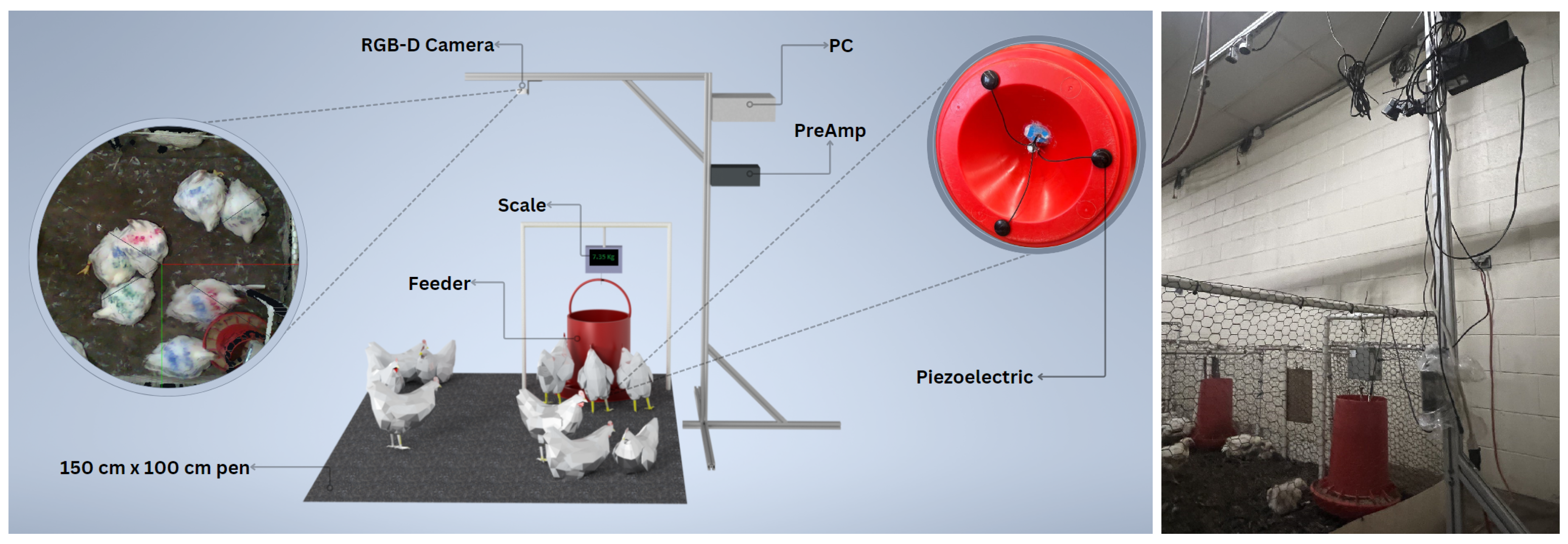
Additionally, an Intel RealSense LiDAR Camera L515 was mounted on top of the pen and scheduled to record 15 min-long videos per hour. Videos were recorded at a 30-frame-per-second sampling rate with a resolution of 1024 × 768 pixels. The data acquisition scripts were run on an Intel NUC with 8 Core™ i7 5.20 GHz Processors, 32 GB of RAM, and 1 TB disk space. The recorded data were then intermittently uploaded to the UT Smart Agriculture Lab’s workstation through a File Transfer Protocol (FTP) connection. The general housing and data acquisition setup is shown in Figure 1. Video recordings were used in the annotation process and for investigating the predicted results.

2.3. Data Annotation and Preprocessing

To train the model, a subset of the raw data containing 36 audio files, 30 s each, was randomly sampled from the whole raw recordings. To learn about the feeding signal pattern, video recordings were chosen such that only one chicken at a time was fed. Then, the corresponding audio recording was found and matched with the video section. After investigating a hundred samples, the feed-pecking signal pattern was distinguishable for the subject matter expert in charge of labeling. Since matching every audio recording with the corresponding video was labor-intensive and time consuming, the remaining samples were labeled by listening to the audio recordings. Thus, audio recordings were annotated using the Label-Studio software by hearing them based on the judgments of the subject matter expert [20]. The final annotated dataset for the training model contained 1949 feed-pecking samples and 1370 non-pecking samples (352 singing and stress calls, 499 anomalies, and 519 silence samples).

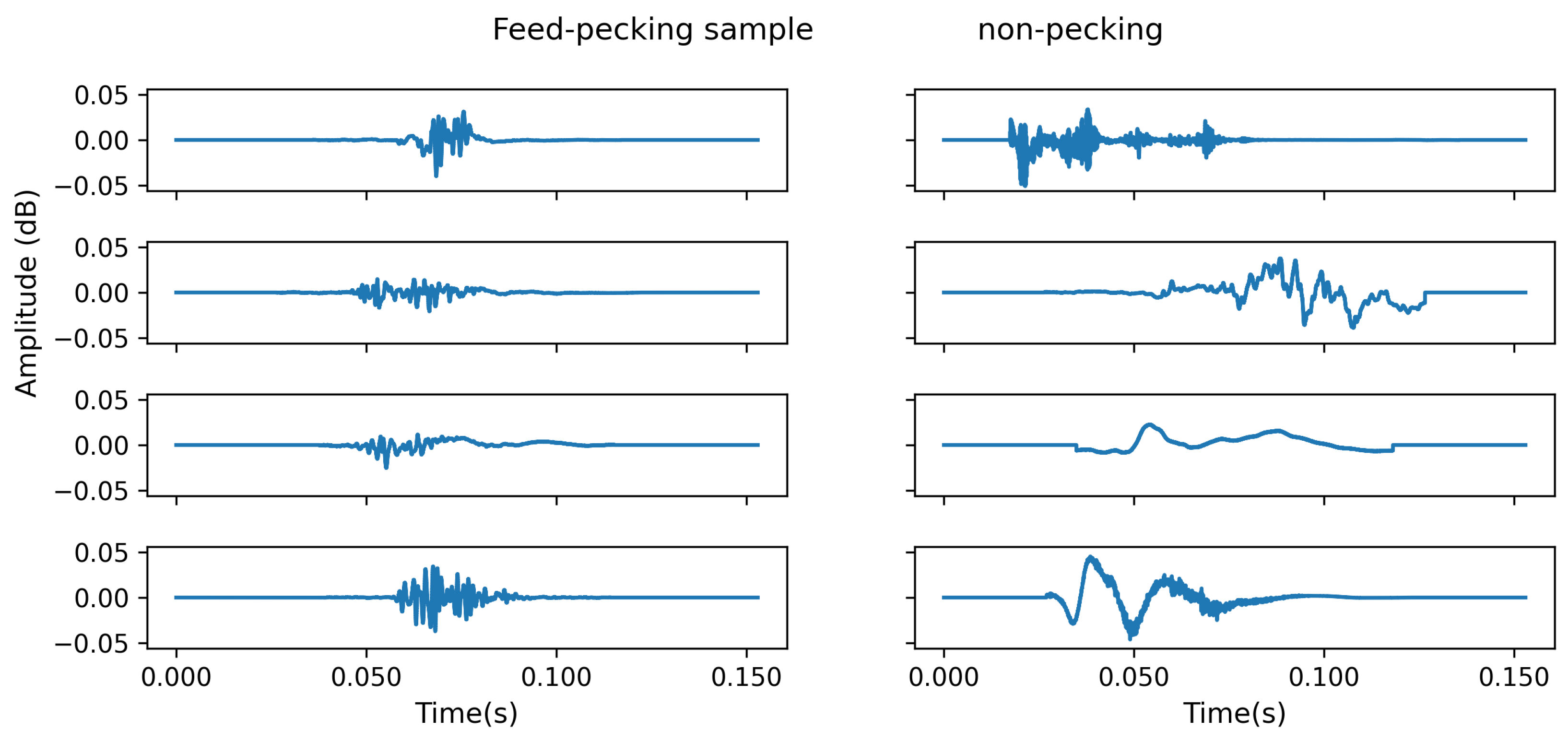
Figure 2 illustrates a few samples of feed-pecking and non-pecking audio events. Sounds created by events such as chickens jumping on or pushing the feeder, leading to a sudden high amplitude, were considered anomaly events. Singing is the sound chickens make while roaming around or feeding, and the stress call is considered the high sudden high pitch sound chickens make mostly when they are frightened for reasons like detecting human presence.

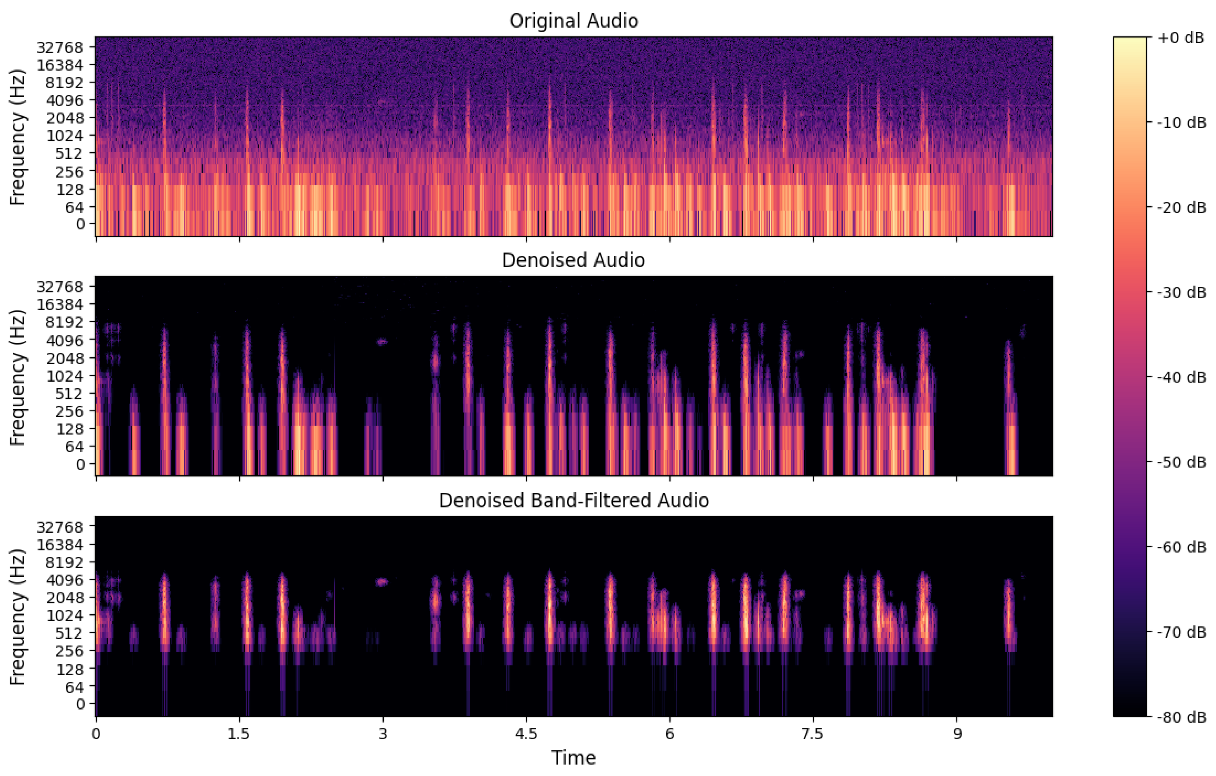
Preparing the dataset before feeding it to the machine learning model is essential for achieving the best results possible. Accordingly, a stationary noise (e.g., ventilation) removal method implemented by Scikit-Maad Python library was first applied to increase the signal-to-noise ratio [21]. After exploring the frequency ranges in audio samples, a band-pass filter was applied to cutoff frequencies ranging from 200 Hz to 4000 Hz. The band-pass filter led to filtering out the redundant high-frequency information as well as low-frequency ambient sounds. Therefore, parts of the signals outside this range were eliminated. Figure 3 shows the result of each audio preprocessing step.

2.4. Model Development

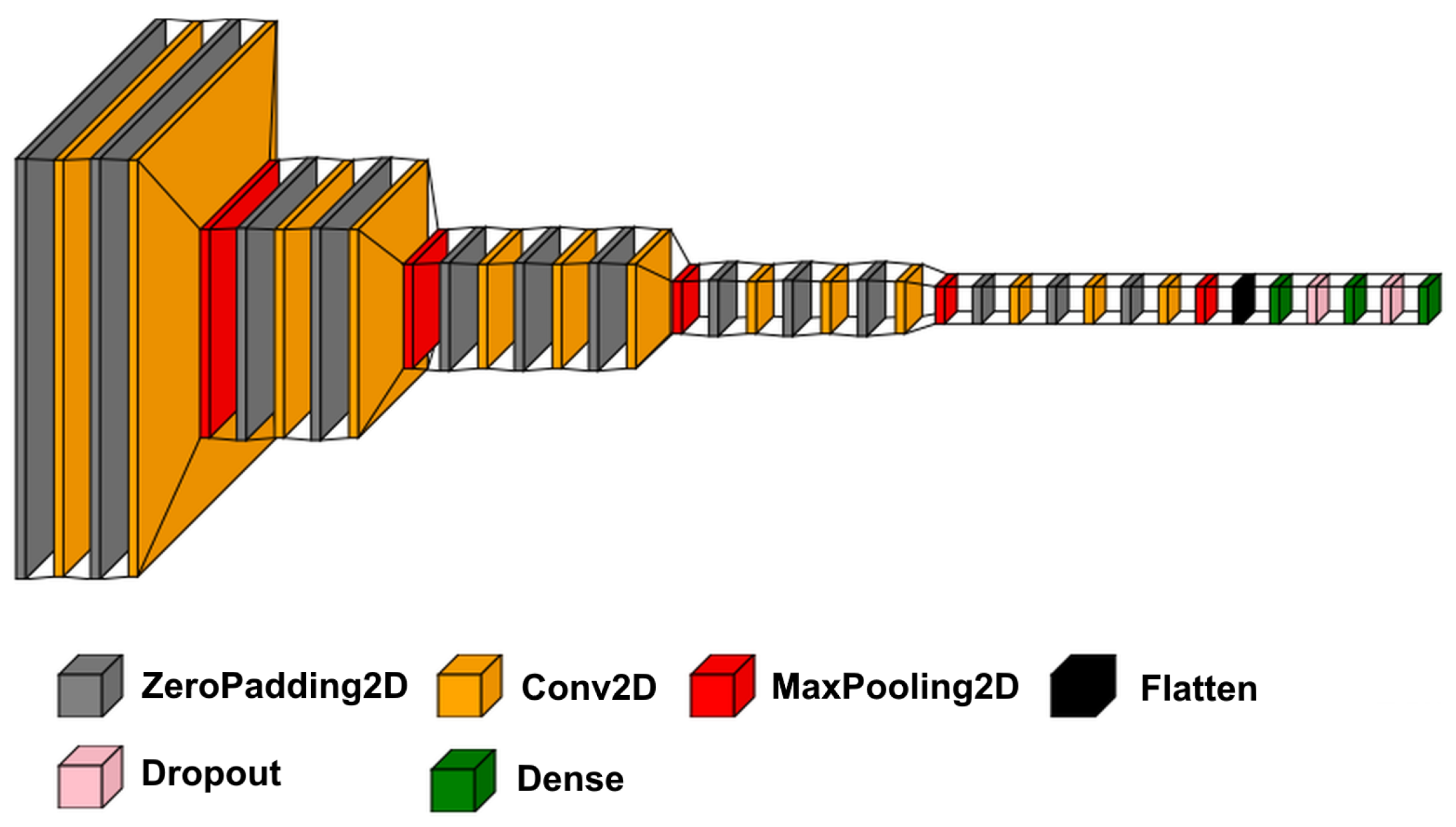
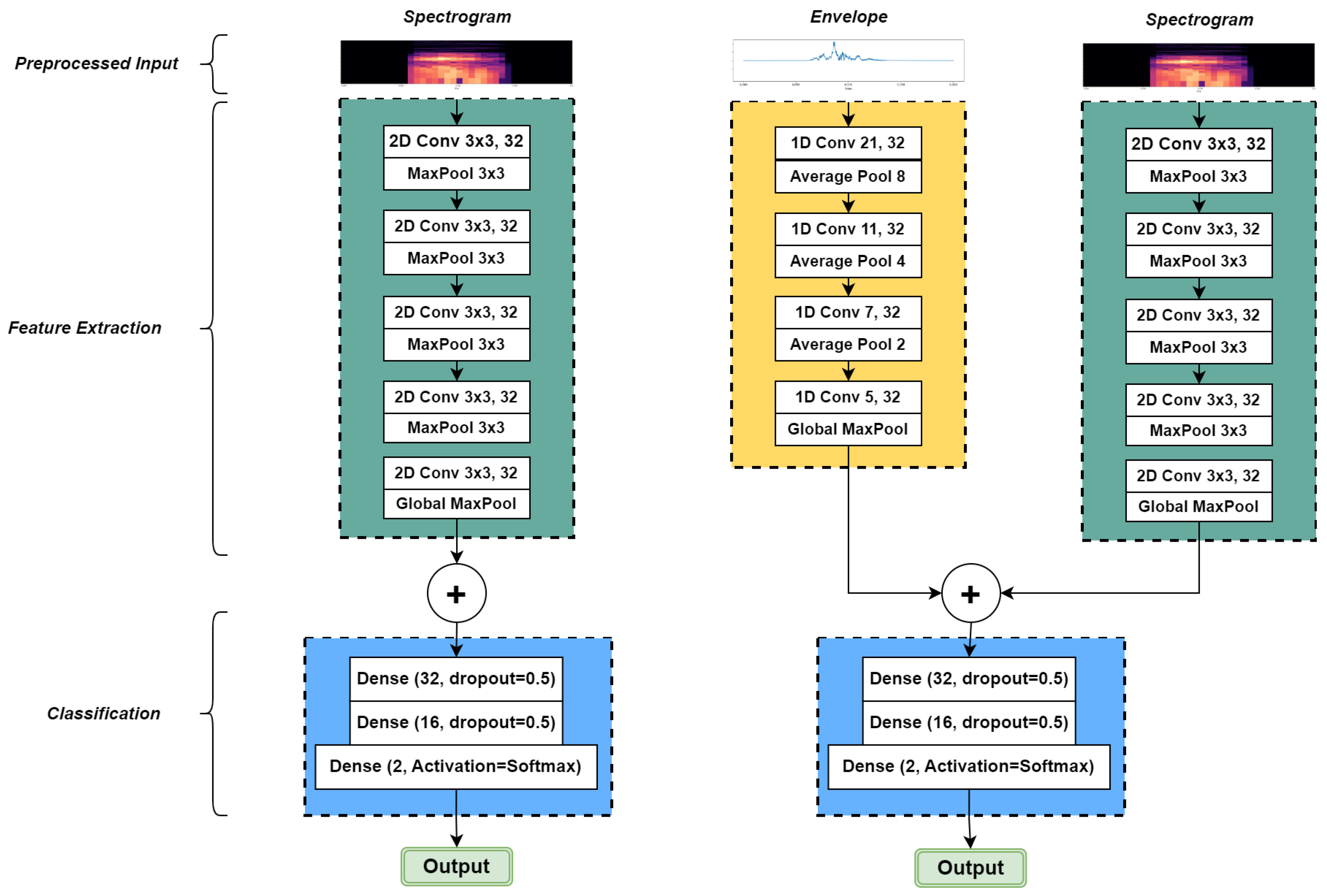
First, we started with the original VGG16 network on the spectrogram data for the binary classification of feed-pecking vs. non-pecking signals (including anomalies, silence, singing, and stress calls). As illustrated in Figure 4, the original VGG16 network has five blocks containing 16 convolutional layers in total. In the first two blocks, two consecutive convolutional layers are stacked up, followed by a MaxPooling layer to downsample the features. The subsequent three blocks have three convolutional layers and the MaxPooling layer. The role of the max-pooling layer was to decrease the dimensions of the input to the layer by considering the highest value in the defined pool window size (receptive field), which led to merging the neighboring features into one, semantically [22]. Eventually, the last layer’s filter bank was flattened and fed to three dense layers for classification purposes. Since this research aimed to develop a low-cost system, we planned to reduce the size of the model so that it can be deployed on a microcontroller-based edge device. Thus, the convolutional layers and the neurons at the dense layers were gradually reduced to minimize the model size as much as possible without compromising the model’s accuracy. Furthermore, since the spectrogram image size was smaller (512 × 38) than the images used to train the original VGG16 model, it was assumed that there were fewer details in these images compared to images in the ImageNet dataset, which made it possible to reduce the model size by only having five blocks, each containing one convolutional layer with a ReLU (rectified linear unit) activation function followed by a max-pooling layer (Figure 5). With a 512 × 38 spectrogram image as the input, the number of parameters for this model was 33,794 (132.01 KB).

Additionally, to take time-domain features into account in the modeling process, another model with an extra branch for 1D audio feature extraction was proposed with the signal envelope as the input to the new branch. In noisy environments like poultry farms, analyzing the signal envelop is an effective way to enhance the processing results by reducing the noise effect in the original signal. Accordingly, the signal envelope was extracted by applying a Hilbert transform on the original signal, and it used as the input for the 1D branch. This branch contained three convolutional layers followed by a max-pooling layer and one convolutional layer followed by a global max-pooling layer. With a 512 × 38 spectrogram image for the 2D branch, and a 9600-element array of the signal envelop for the 1D branch, as the inputs, the total number of parameters for the final model was 64,306 (251.20 KB).

In the last step (classification section in Figure 5), the extracted features were concatenated and fed to two dense layers with 32 and 16 neurons and a 0.5 dropout rate. Dropout layers helped the model prevent overfitting by randomly deactivating a percentage of neurons in dense layers in each training pass, leading to a more reliable generalization performance [18]. Finally, the last dense layer had two neurons with the SoftMax activation function corresponding to the possibility of each detected class.

2.5. Model Validation

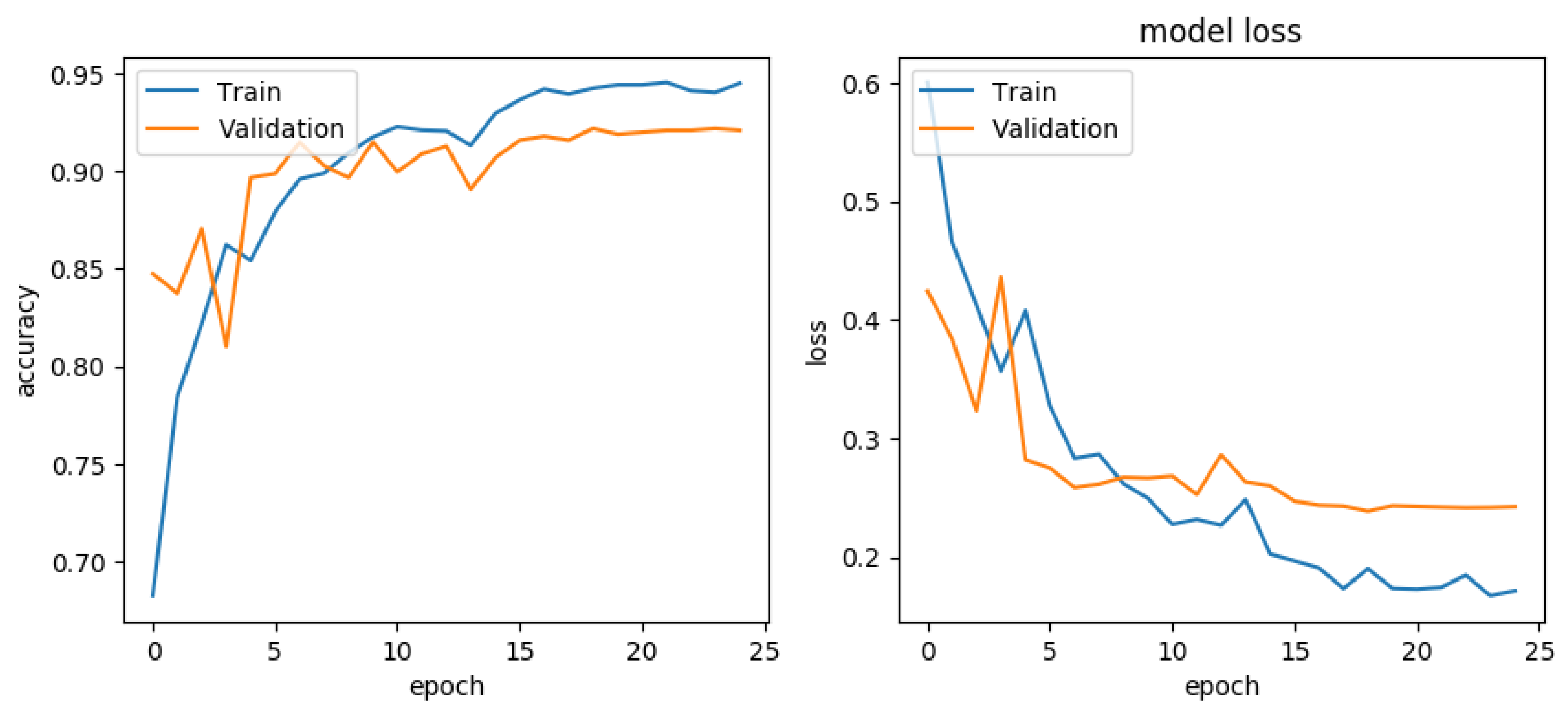
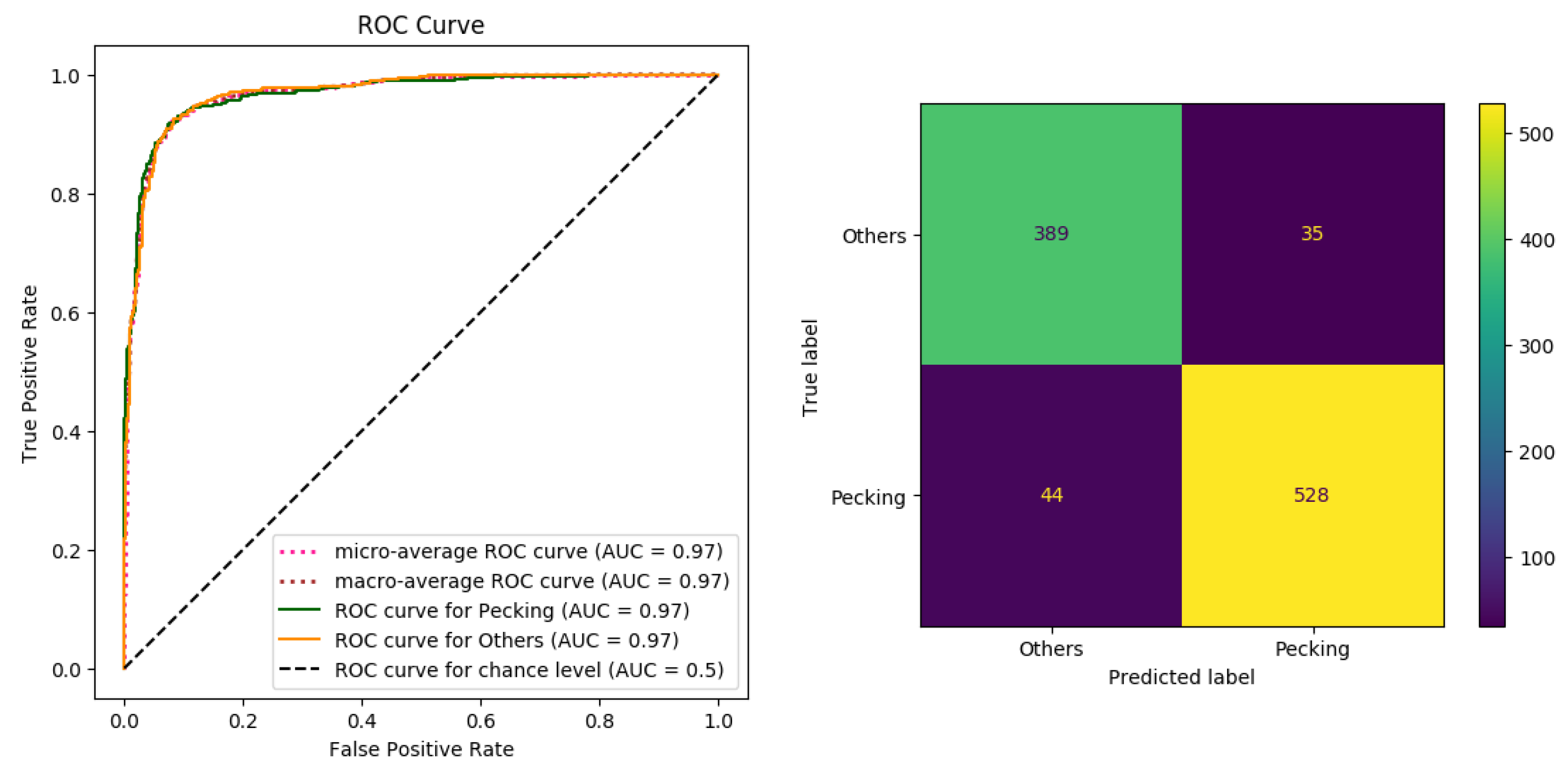
Model training and evaluations are another critical step in a machine learning pipeline. The correct measure of accuracy is assessed based on the model’s performance on unseen samples. Accordingly, 80% of the dataset, including 2655 samples, was used for training the model, and the accuracy was evaluated using the remaining 20% of the dataset containing 664 unseen samples as the test set. Next, both models were trained on the training set for 30 epochs with a batch size of 40 using the binary cross entropy loss function. The learning rate was scheduled to decrease by a factor of 10 after 15 epochs. After the training process, test set samples were classified using the model, and results, including the number of true positive (TP), true negative (TN), false positive (FP), and false negative (FN), were used to construct the confusion matrix. Diagonal values in a confusion matrix show the truly classified samples; the off-diagonal values are the misclassified samples. The main metrics utilized to evaluate the models’ performance were accuracy, precision, recall, f1-score, and Area Under the Curve (AUC) of the Receiver Operating Characteristic (ROC) curve. These metrics were extracted based on the values in the confusion matrix as follows:

$$\mathrm{Precision}=\frac{\mathrm{TP}}{\mathrm{TP}+\mathrm{FP}}$$

(1)

$$\mathrm{Accuracy}=\frac{\mathrm{TP}+\mathrm{TN}}{\mathrm{TP}+\mathrm{TN}+\mathrm{FP}+\mathrm{FN}}$$

(2)

$$\mathrm{Recall}=\frac{\mathrm{TP}}{\mathrm{TP}+\mathrm{FN}}$$

(3)

$$\mathrm{F}1-\mathrm{score}=\frac{2\times \mathrm{TP}}{2\times \mathrm{TP}+\mathrm{FP}+\mathrm{FN}}$$

(4)

$$\mathrm{AUC}=\frac{1}{2}\left(\frac{\mathrm{TP}}{\mathrm{TP}+\mathrm{FN}}+\frac{\mathrm{TN}}{\mathrm{TN}+\mathrm{FP}}\right)$$

(5)

Finally, the proposed models were compared based on the metrics mentioned above, and the model showing a higher performance was chosen for processing the dataset and estimating the feed consumption.

2.6. Feed Consumption Analysis

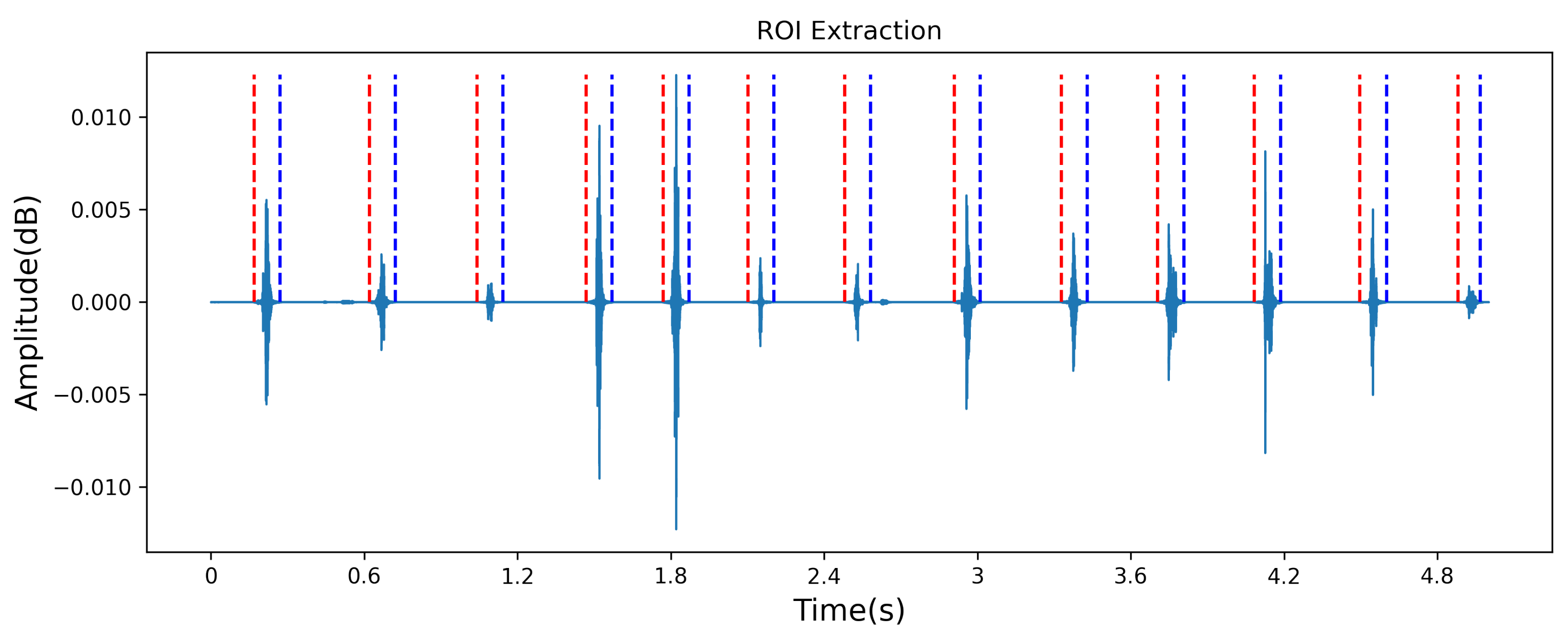
The raw data containing 432 h (19 days) of audio recordings were processed to evaluate the proposed method. Then, the calculated feed consumptions were compared with the actual consumptions recorded by the weighting scale. To process the whole dataset, every audio file was loaded into the memory and preprocessed using the same pipeline described in the preprocessing section. Each audio file was processed using the Scikit-Maad Python library [21] to find candidate audio segments extracted by a continuous wavelet transform (CWT)-based method [24] within the defined range of frequency between 200 Hz and 4000 Hz as shown in Figure 6. Next, the extracted ROIs (Regions of Interest) were fed to the developed model, and the number of feed-pecking in each audio recording was stored in the memory.

The number of classified feed-pecking events in each audio recording was counted and aggregated for each hour. A former study reported that each feed-pecking action by broiler chickens would take about 0.025 g of feed on average [11]. Therefore, the final estimated feed consumption was calculated as follows:

$$\mathrm{Feed} \mathrm{Consumption}=\mathrm{FIPP}\times \mathrm{NP}$$

(6)

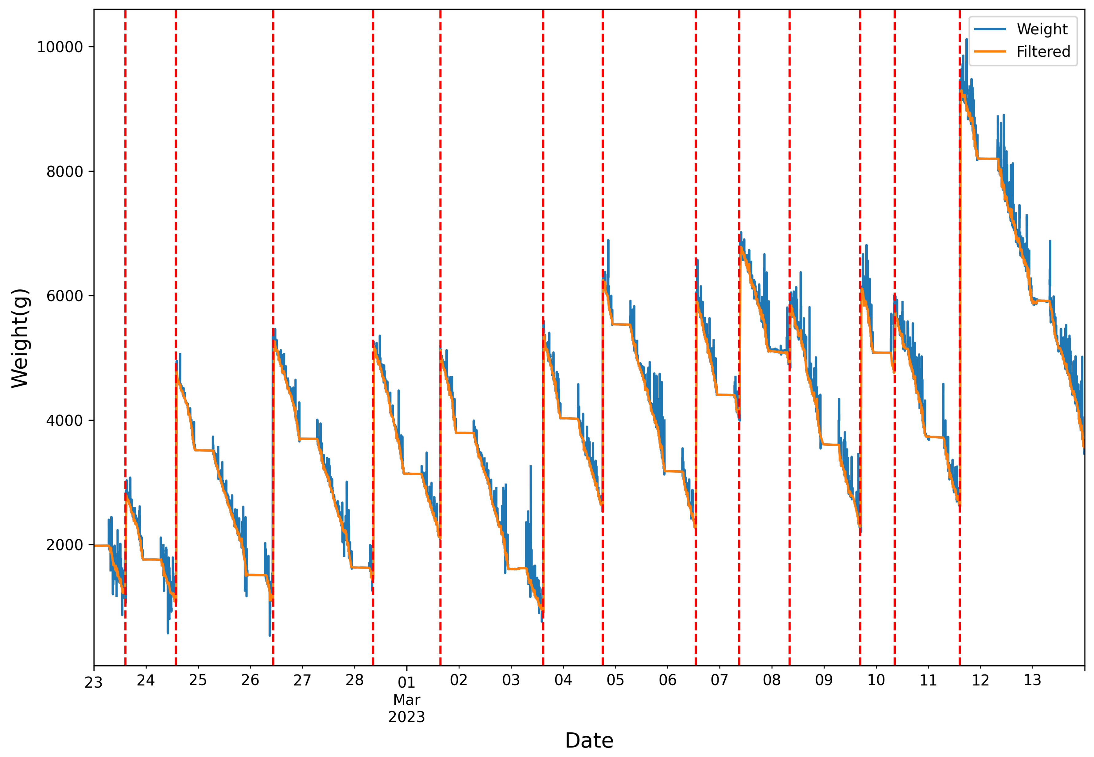
where the FIPP is the constant value of 0.025 g for feed intake per peck, and NP is the total number of pecking events detected by the model per audio sample, used as an estimate of feed consumption at the feeder during the recording period. This estimate may reflect the activity of one or multiple chickens at the feeder. To compare the estimated feed consumption by the proposed method and the ground truth data, the noise in scale measurements was removed as the first step by applying a Hampel filter [25] with a window size of 100 samples followed by a rolling min filter with a window size of 10 samples (Figure 7). Then, a piece-wise linear regression model was applied to each day’s data, and the difference between the feed measure from the beginning and the end of each hour was considered the consumption value provided by the scale data [26]. Since the feeder was frequently refilled, the line segments with ascending slopes were considered refill events and ignored in the calculations.

In the final step, the Pearson product moment correlation coefficient (PPMCC) was used as a statistical method to measure the linear correlation between the two variables. The range of the PPMCC values is −1 to 1. The positive value of PPMCC shows the degree to which the variables are linearly associated. Conversely, zero and negative values show no linear correlation and negative correlation, respectively [27].

$$\mathrm{PPMCC}=\frac{Cov(x,y)}{{\sigma }_x+{\sigma }_y}$$

(7)

where $Cov$ is the covariance of the two variables, and ${\sigma }_x$ and ${\sigma }_y$ are the standard deviations of the variables x and y, respectively. Furthermore, the coefficient of determination ($R^2$ score) between the two variables was calculated to assess the degree of variability explained by the model, which is defined as:

$$R^2=1-\frac{\mathrm{SSres}}{\mathrm{SStot}}$$

(8)

where the SStot and SSres are the total sum of squares, and the sum of squares of residuals, respectively.

3. Results

3.1. Model Validation

Nineteen days of continuous audio recordings were acquired during this study, among which 36 samples were randomly picked, each containing 30 s audio. In each sample, feed-pecking and non-pecking events (including anomaly, singing, and silence) were labeled, resulting in 1949 feed-pecking and 1370 non-pecking events used for the model development process. Both models were trained for 25 epochs where the training and validation accuracy met a plateau. A batch size of 40 were chosen for the training process. Adam optimizer was used to train the models, and the best-performing model was saved with the corresponding epoch number. Next, the models’ performance related to each metric was assessed by feeding the unseen samples from the test set, leading to the results shown in

Table 1. Models’ performance on the test set: Model A only used spectrogram data as input, whereas Model B is the model with both the audio signal’s envelop and the spectrogram as inputs.

Model	Class	Accuracy	Precision	Recall	F1-Score	AUC	Parameters
A	Feed-Pecking	0.90	0.93	0.91	0.92	0.96	33,794
A	Others	0.89	0.89	0.90	0.89	0.96
A	Average per-class	0.89	0.91	0.90	0.90	0.96
B	Feed-Pecking	0.94	0.94	0.92	0.93	0.97	64,306
B	Others	0.90	0.90	0.92	0.91	0.97
B	Average per-class	0.92	0.92	0.92	0.92	0.97

.

Based on the provided results, the model B with both the envelope and the spectrogram as inputs outperformed the other model in all metrics. Accordingly, model B was chosen for the rest of the research. Note that compared to the original VGG16 with approximately 138 million parameters, the proposed model is drastically reduced in size, resulting in a more suitable model to deploy on edge devices while mitigating for overfitting due to a lower model complexity. Figure 8 illustrates the training and validation accuracy and loss of the selected model for each epoch. The model’s accuracy converged after 20 epochs and the best fit occurred at the 19th epoch with 94% validation accuracy. Figure 9 shows the extracted confusion matrix and the model’s ROC curve from the classification results on the test set. The developed model could accurately classify 528 feed-pecking events out of 572 samples with an accuracy of 94% and an f1-score of 93%. Also, the ROC curves for both classes were dragged toward the plot’s upper left corner, indicating high AUC values.

The calculated metrics for model evaluation on the test set were extracted from the confusion matrix containing the precision, recall, f1-score, and AUC, and are shown in Table 1. The trained model achieved an overall classification accuracy of 92%, and the average per-class classification accuracy was 92%.

3.2. Feed Consumption Analysis

Processing 1824 audio files took about 410 min, with an average of 22 s of processing time for each 15 min audio recording. The number of feed-pecking in each processed recording was timestamped and mapped to the feed consumption recorded by the scale with the same timestamp, providing the proper format to compare the estimation results with the ground truth data obtained from the weight measurement device as illustrated in Figure 10. The PPMCC correlation and R2 score between these measures were 85% and 71%, respectively. To further investigate the source of the error in our method, the mean absolute error of each hour was calculated for the entire duration of 19 days, illustrated in Figure 11. The hourly mean absolute error (MAE) between the proposed feed intake estimation algorithm and the scale measures (as the reference method) exhibits a distinct pattern throughout the day. The estimation error during the night was close to zero, which was expected, as the chickens were inactive. Nevertheless, the error distribution fluctuated during the rest of the day, with a slight increase early in the morning (between 7 and 9 a.m.) as indicated by the green box plots, in the noon (between 1 and 3 p.m.), and a steep increase late at night (between 8 and 10 p.m.) before the lights were turned off.

This suggests that the algorithm performs well in estimating feed intake during this period. However, as the day progresses, the MAE gradually increases, with the box plots transitioning to blue, purple, and eventually red colors. The highest errors seem to occur around midday and the late afternoon/evening hours. This pattern may be attributable to factors such as variations in animal behavior, environmental conditions, or other factors that could influence the accuracy of the algorithm during different times of the day. Note that the diamonds in the plot represent outliers in the data for each time period. These outliers are data points that fall outside the whiskers of the box plots. These outliers suggest that while the majority of error measurements followed a predictable pattern, there are frequent instances of unusually high errors. These happened particularly during the peak hours where the estimation error was relatively higher possibly due to several chickens feeding at the same time.

To perform a comparison with the method proposed in previous study by Aydin et al. [12], the feed consumption estimates are compared with the scale measures as the reference method in terms of relative error rate.

4. Discussion

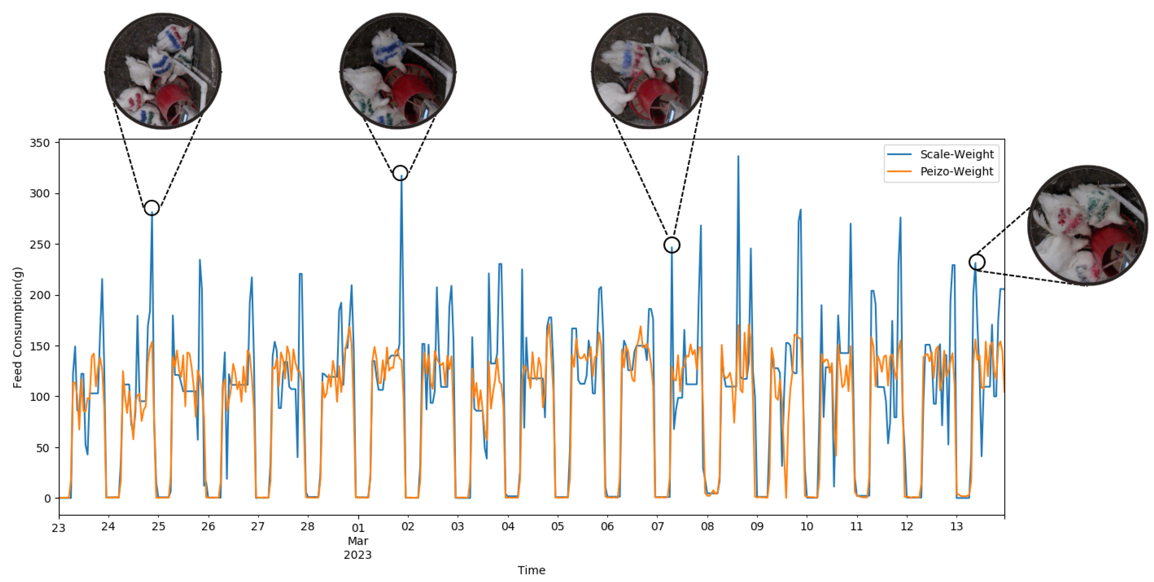
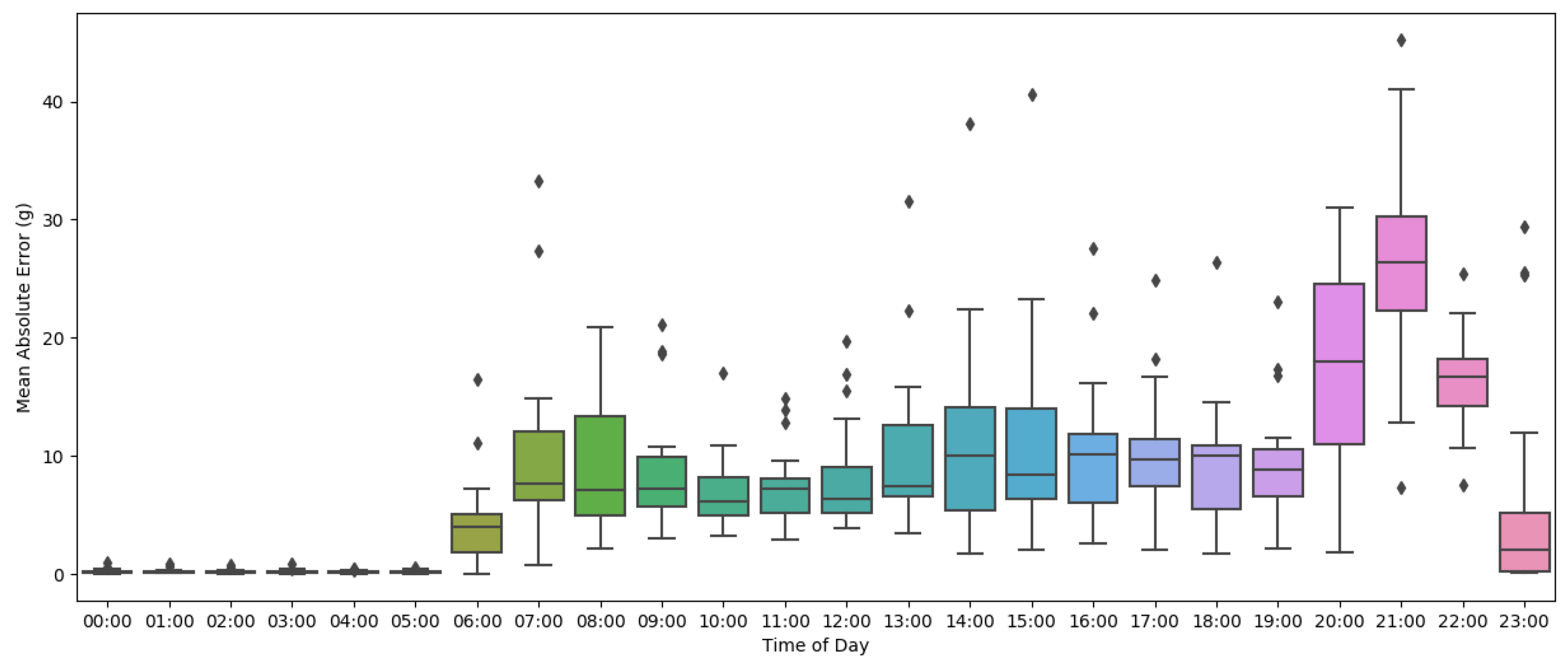
Based on the extracted results, the proposed method could capture the flock’s consumption trend with a relatively high correlation except for the early mornings and late nights, which appeared to have a sudden increase in feed intake. Video recordings were checked to find the reason behind the peaks in feed consumption error at certain hours of each day. Investigating the videos during the peak hours, as illustrated in Figure 10, we found that the feeder was surrounded by several chickens pecking simultaneously, which caused model estimation to decrease slightly. This pattern might indicate meal patterns during the day, which means more chickens were eating at certain time periods. Overlapping feed-pecking events in the audio signal was likely a reason for the drop in model estimation accuracy in certain hours. Based on the results provided in

Table 2. Daily feed intake estimation results.

Day	NPPD 1	Feed Intake Scale (g)	Feed Intake Algorithm (g)	Absolute Error (g)	Error (%)
1	70,895	1772.4	1801.9	29.5	1.6
2	65,261	1631.5	1994.8	363.3	18.2
3	77,839	1946.0	1913.2	32.8	1.7
4	73,349	1833.7	1943.7	110.0	5.7
5	81,668	2041.7	2067.7	26.0	1.3
6	79,549	1988.7	2306.2	317.5	13.8
7	84,582	2114.6	2324.0	209.4	9.0
8	81,630	2040.8	2091.0	50.2	2.4
9	66,396	1659.9	2042.3	382.4	18.7
10	81,620	2040.5	2138.0	97.5	4.6
11	89,769	2244.2	2365.0	120.8	5.1
12	90,458	2261.5	2403.3	141.8	5.9
13	84,959	2124.0	2057.2	66.8	3.2
14	82,880	2072.0	2475.4	403.4	16.3
15	72,404	1810.1	2377.7	567.6	23.9
16	77,401	1935.0	2305.2	370.1	16.1
17	86,289	2157.2	2246.6	89.4	4.0
18	85,272	2131.8	2229.4	97.6	4.4
19	87,409	2185.2	2407.4	222.2	9.2
Mean	79,980.5	1999.5	2183.7	194.6	8.7
STD	7407.8	185.2	194.6	159.5	7.0

¹ NPPD: number of feed-peckings per day.

, the proposed method showed a mean 8.70 ± 7.0% percent error on daily feed intake estimation. However, the absolute error on some days, like the 15th and 14th, showed high values of 567 g and 403 g, which led to a relatively high standard deviation of 7% percent.

Although the accuracy could be improved, one advantage of our proposed method is that a cheap 3-in-1 contact piezoelectric sensor was used instead of an off-the-shelf microphone, compared to similar studies conducted by Aydin et al. [11,12]. Using the 3-in-1 piezoelectric sensor had the advantage of properly covering the feeder, which led to a more consistent, higher-quality sound compared to one microphone, where the signals near it would have higher amplitude and signals on the other side of the feeder would be weaker, if detectable at all. We would like to point out that most of the devices included in the materials were only for system development and evaluation. The final audio-based sensing system is expected to only include the piezoelectric sensor and a micro-controller. Also, a deep learning-based classifier was developed and used, leading to a more robust classification performance of 94% accuracy for feed-pecking and 90% for non-pecking events, respectively. Furthermore, thanks to the developed model, the estimated feed intake showed a lower error percentage of 8%, which shows a 5% improvement compared to a similar previous work [12] with a 14 ± 3% error. Last but not least, this study was unprecedentedly performed for 19 days (24/7), which provided more reliable and realistic data and more robust results and benchmarking since it included refill events, anomalies, different feed levels in the feeder, and meal patterns.

5. Future Works

First, although the proposed method achieved improved accuracy in feed intake estimation compared to similar previous works, there is still a lot of room to improve the model performance on anomaly detection by training it on more data. Furthermore, as discussed in the previous section, having several chickens feeding at the same time can reduce the accuracy of the feed intake estimation. Increasing the sampling rate might address this issue by providing higher resolution in audio events, which require custom-designed hardware based on embedded systems to acquire high-resolution audio recordings. Also, given the three piezoelectric sensors attached to the feeder, we can potentially triangulate the approximate location of pecking events to be able to distinguish between different feed-pecking events at the same time. Second, based on observing video recordings, another critical factor to consider is the feed level in the feeder. As the feed level changes over time, it might contribute to the increase in the overall error because when the feed level is relatively low, feed-pecking events have more intense amplitudes, which may lead to a higher probability of feed-pecking misclassification as others (more specifically as anomalies). Thus, training the model with more data or using a feeder that has more consistent feed levels should be performed in future studies.

Third, with recent advancements in processing power and AI accelerator chips on micro-controller devices, it is possible to implement the proposed method on an affordable low-power embedded system and deploy it on a commercial farm scale connected to the cloud, providing an AI-enabled management system for the farmers. Our team will continue to improve and refine our device to move towards a more practical device for commercial use.

Last, most commercial farms use straight-line chain feeder systems, which are different from the hanging feeders in this study. The proposed method, although it used a hanging feeder, can be applied to a commercial feeder pan. However, further studies should be conducted to validate this hypothesis.

6. Conclusions

Feed intake monitoring plays a prominent role in understanding poultry feeding behavior. It provides valuable insight into poultry farm management and may help improve the feed conversion ratio. In this research, a low-cost system was proposed based on the audio signals captured by piezoelectric sensors mounted at the bottom of a feeder to estimate the feed consumption based on the number of feed-pecking events that happened. Nineteen (19) consecutive days of audio data were recorded, and a randomly sampled part of the dataset was labeled for model development. A CNN-based deep learning model with two inputs (including the audio envelope and the spectrogram) was developed to classify feed-pecking events from non-pecking events (silence, signing, stress class, and anomalies). The model achieved 94% accuracy in feed-pecking detection, with a 92% overall accuracy. Processing the whole 19 days of data and counting detected feed-pecking events using the developed model showed a 5% decrease in feed intake estimation mean percent error compared to the previous work. Moreover, a correlation of 85% and a 71% R2 score between the estimated feed consumption and the ground truth feed consumption was achieved in this study. According to the results, the proposed system can be further investigated as a method to measure broiler feed intake at each feeder pan as a low-cost feed intake monitoring tool.