
Improving Coffee Yield Interpolation in the Presence of Outliers Using Multivariate Geostatistics and Satellite Data

 ,
,  , and
, and 
Abstract
1. Introduction
2. Materials and Methods
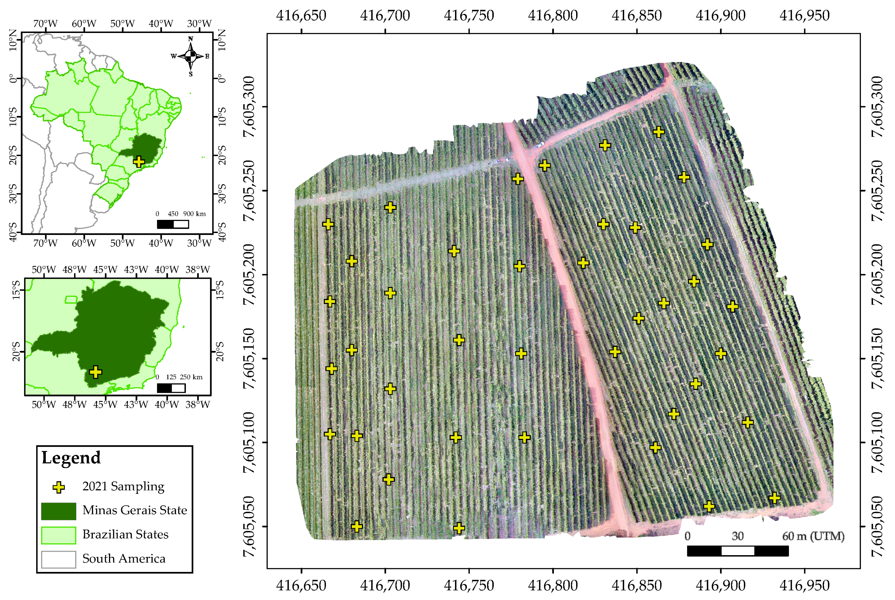
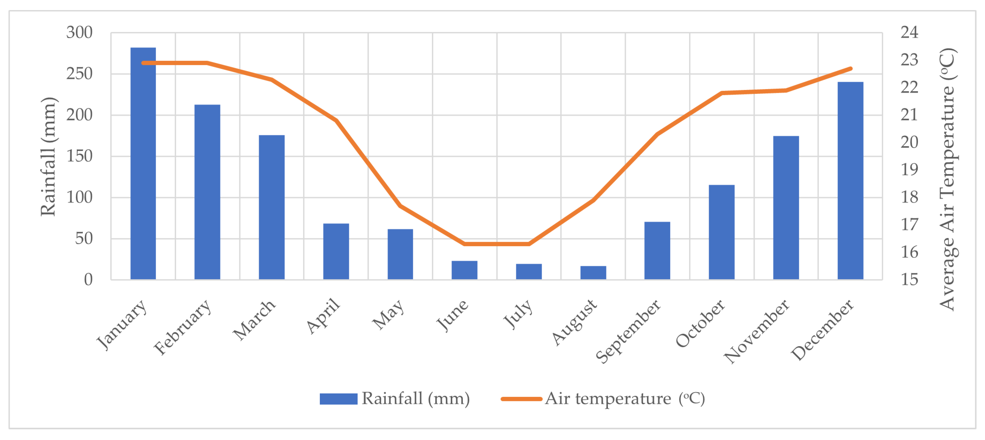
2.1. Description of the Study Site and Agronomic Practices
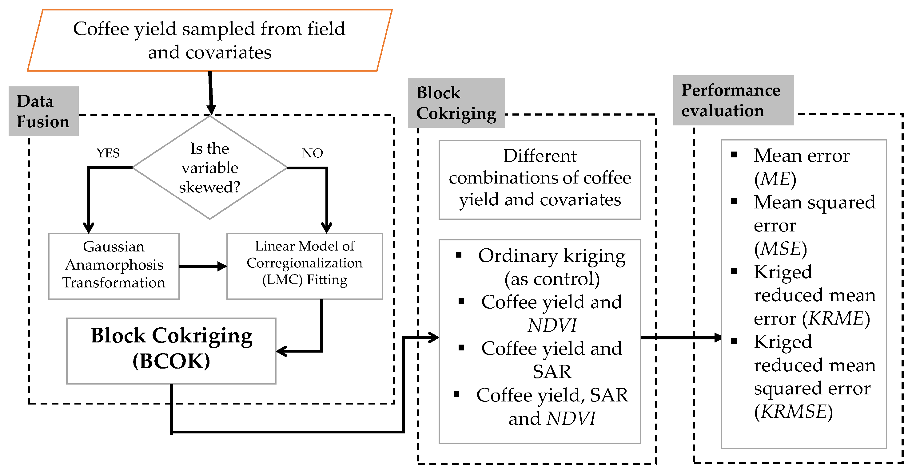
2.2. Multivariate Geostatistics
2.2.1. Preprocessing with Gaussian Anamorphosis Transformation
2.2.2. Fitting of Linear Model of Co-Regionalization (LMC)
2.2.3. Block Cokriging (BCOK)
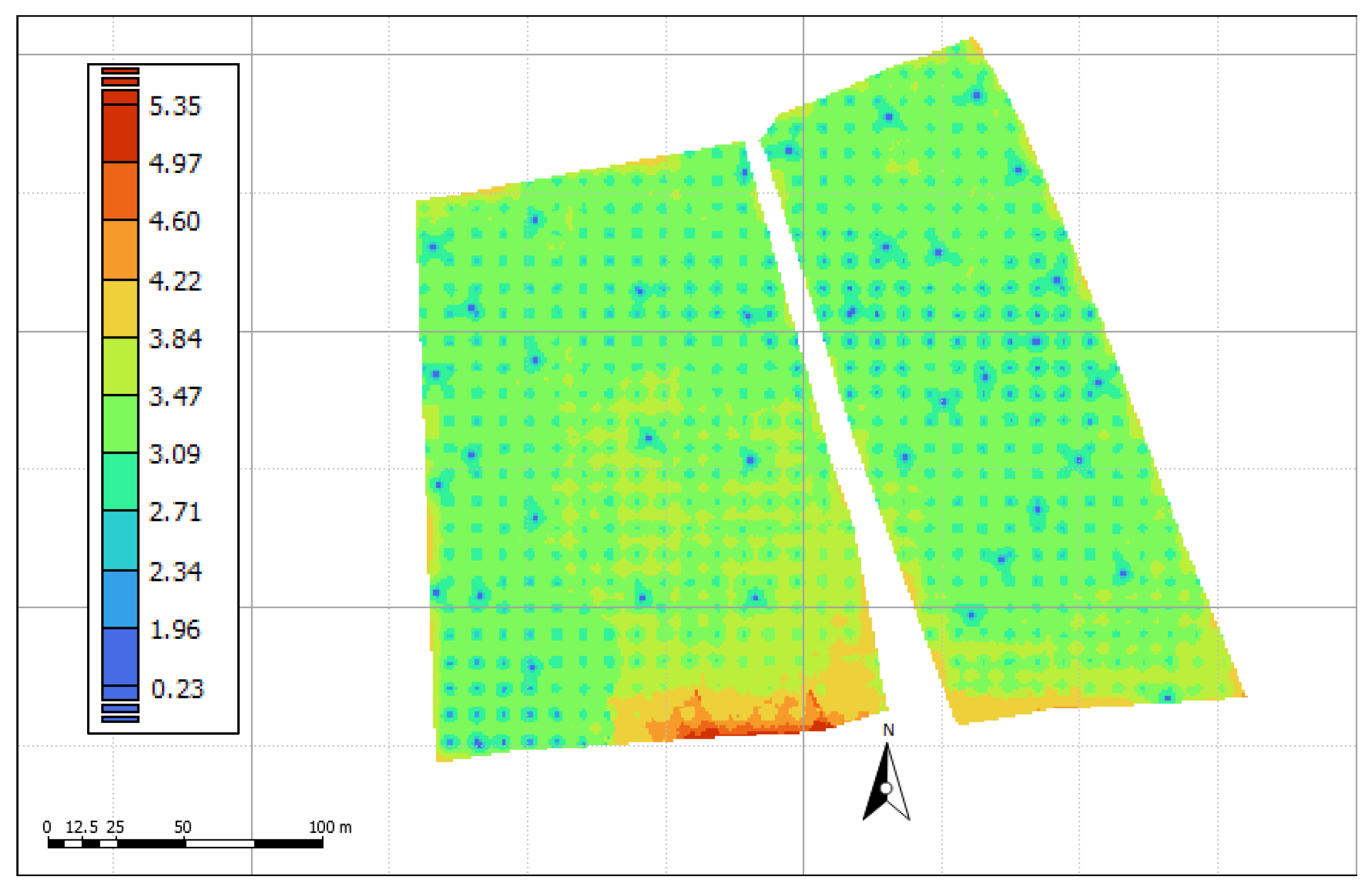
2.3. NDVI and SAR Mosaic Derivation from Sentinel-1 and -2
2.4. Performance Evaluation
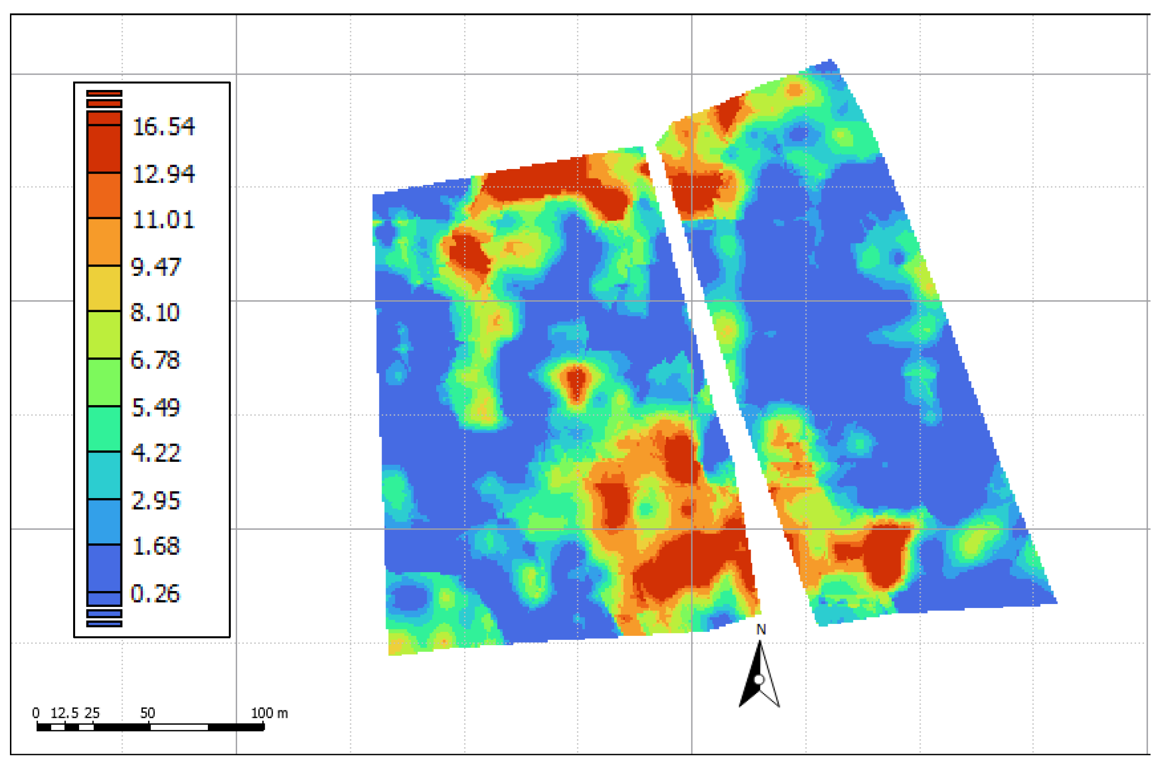
3. Results and Discussion
4. Conclusions and Recommendation
Author Contributions
Funding
Data Availability Statement
Acknowledgments
Conflicts of Interest
Abbreviations
| PA | Precision agriculture |
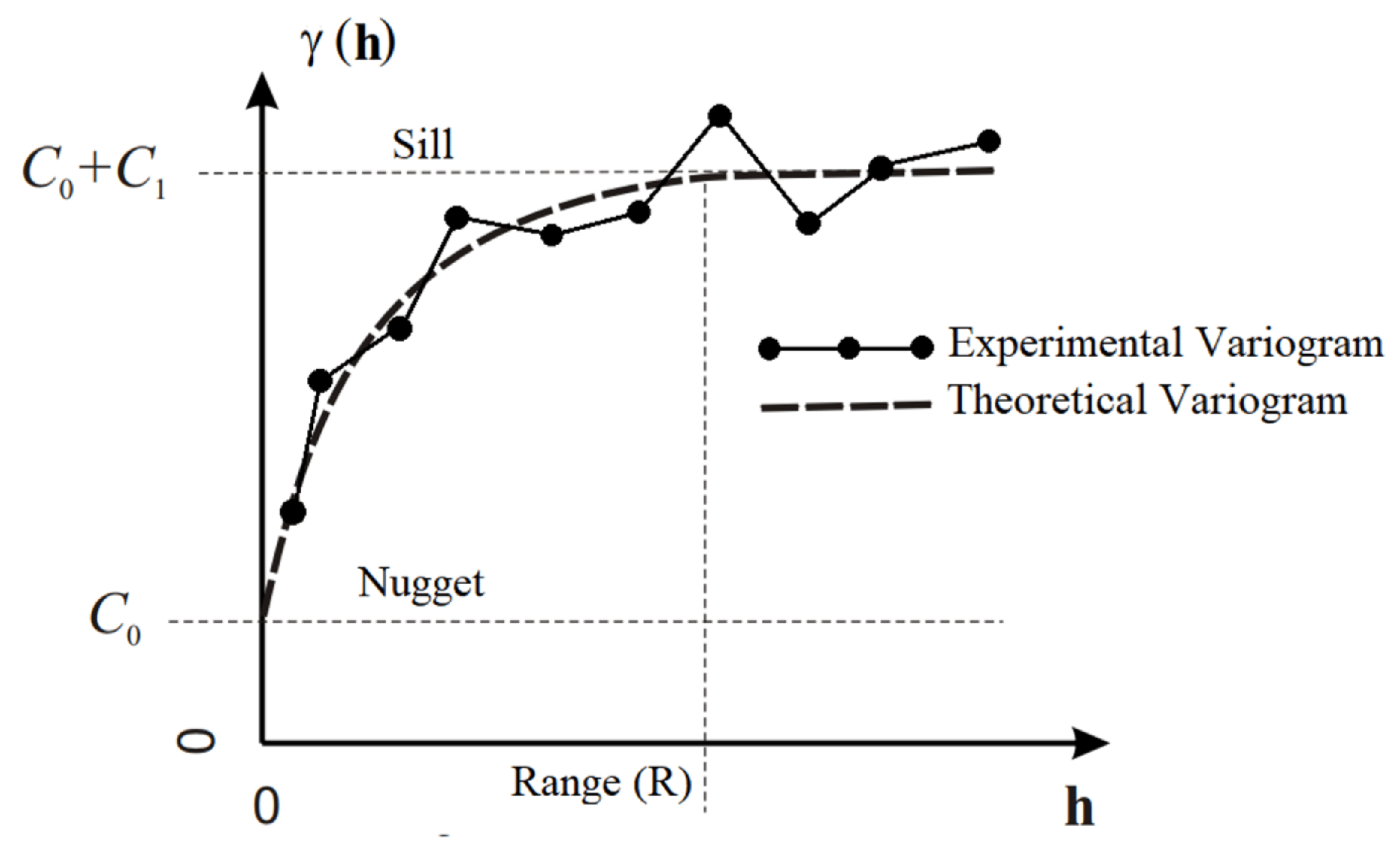
| R | Range |
| Nugget effect | |
| Spatial dependence degree | |
| Sill or structural component | |
| OK | Ordinary kriging |
| BCOK | Block cokriging |
| LMC | Linear model of co-regionalization |
| NDVI | Coefficient of variation |
| SAR | Synthetic Aperture Radar |
| SD | Standard deviation |
| KRMSE | Kriged reduced mean squared error |
| KRME | Kriged reduced mean error |
| MSE | Mean squared error |
| ME | Mean error |
| Min | Minimum value |
| Max | Maximum value |
| N | Number of observations |
References
- Carvalho, L.G.d.; Sediyama, G.C.; Cecon, P.R.; Alves, H.M. A regression model to predict coffee productivity in Southern Minas Gerais, Brazil. Rev. Bras. Eng. Agrícola Ambient. 2004, 8, 204–211. [Google Scholar] [CrossRef]
- Johnson, M.A.; Ruiz-Diaz, C.P.; Manoukis, N.C.; Verle Rodrigues, J.C. Coffee berry borer (Hypothenemus hampei), a global pest of coffee: Perspectives from historical and recent invasions, and future priorities. Insects 2020, 11, 882. [Google Scholar] [CrossRef] [PubMed]
- Mayoli, R.N.; Gitau, K. The effects of shade trees on physiology of arabica coffee. Afr. J. Hort. Sci. 2012, 6, 35–42. [Google Scholar]
- Sakai, E.; Barbosa, E.A.A.; de Carvalho Silveira, J.M.; de Matos Pires, R.C. Coffee productivity and root systems in cultivation schemes with different population arrangements and with and without drip irrigation. Agric. Water Manag. 2015, 148, 16–23. [Google Scholar] [CrossRef]
- Souza, Z.M.d.; Marques Júnior, J.; Pereira, G.T.; Moreira, L.F. Variabilidade espacial do pH, Ca, Mg e V% do solo em diferentes formas do relevo sob cultivo de cana-de-açúcar. Ciência Rural 2004, 34, 1763–1771. [Google Scholar] [CrossRef]
- Vieira, H.D. Café Rural; Interciência/FAPERJ: Rio de Janeiro, Brazil, 2017. [Google Scholar]
- Camargo, A.P.; Camargo, M.B.P. Definition and outline for the phenological phases of arabic coffee under Brazilian tropical conditions. Bragantia 2001, 60, 65–68. [Google Scholar] [CrossRef]
- Bernardes, T.; Moreira, M.A.; Adami, M.; Giarolla, A.; Rudorff, B.F.T. Monitoring biennial bearing effect on coffee yield using MODIS remote sensing imagery. Remote Sens. 2012, 4, 2492–2509. [Google Scholar] [CrossRef]
- ISPAG. Precision Ag Definition. Available online: https://www.ispag.org/about/definition (accessed on 18 September 2023).
- Silva, C.d.O.F.; Manzione, R.L.; Oliveira, S.R.d.M. Exploring 20-year applications of geostatistics in precision agriculture in Brazil: What’s next? Precis. Agric. 2023, 24, 2293–2326. [Google Scholar] [CrossRef]
- Juang, K.W.; Lee, D.Y. Comparison of three nonparametric kriging methods for delineating heavy-metal contaminated soils. J. Environ. Qual. 2000, 21, 197–205. [Google Scholar] [CrossRef]
- Lloyd, C.; Atkinson, P.M. Assessing uncertainty in estimates with ordinary and indicator kriging. Comput. Geosci. 2001, 27, 929–937. [Google Scholar] [CrossRef]
- Webster, R.; Oliver, M.A. Geostatistics for Environmental Scientists; John Wiley & Sons: Hoboken, NJ, USA, 2007. [Google Scholar]
- Oliver, M.A.; Webster, R. Basic Steps in Geostatistics: The Variogram and Kriging; Springer: New Jersey, NY, USA, 2015. [Google Scholar]
- Emadi, M.; Shahriari, A.R.; Sadegh-Zadeh, F.; Jalili Seh-Bardan, B.; Dindarlou, A. Geostatistics-based spatial distribution of soil moisture and temperature regime classes in Mazandaran province, northern Iran. Arch. Agron. 2016, 62, 502–522. [Google Scholar] [CrossRef]
- Castrignanò, A.; Buttafuoco, G.; Quarto, R.; Parisi, D.; Rossel, R.V.; Terribile, F.; Langella, G.; Venezia, A. A geostatistical sensor data fusion approach for delineating homogeneous management zones in Precision Agriculture. Catena 2018, 167, 293–304. [Google Scholar] [CrossRef]
- Goovaerts, P. Geostatistics for Natural Resources Evaluation; Oxford University Press: New York, NY, USA, 1997. [Google Scholar]
- Goovaerts, P. Geostatistics in soil science: State-of-the-art and perspectives. Geoderma 1999, 89, 1–45. [Google Scholar] [CrossRef]
- Yost, R.; Uehara, G.; Fox, R. Geostatistical analysis of soil chemical properties of large land areas. II. Kriging. Soil Sci. Soc. Am. J. 1982, 46, 1033–1037. [Google Scholar] [CrossRef]
- Cressie, N. Fitting variogram models by weighted least squares. J. Int. Assoc. Math. Geol. 1985, 17, 563–586. [Google Scholar] [CrossRef]
- Rhif, M.; Ben Abbes, A.; Martinez, B.; Farah, I.R. A deep learning approach for forecasting non-stationary big remote sensing time series. Arab. J. Geosci. 2020, 13, 1174. [Google Scholar] [CrossRef]
- Hu, J.; Zhang, L.; Lee, C.; Gui, R. Advanced big SAR data analytics and applications. Front. Environ. Sci. 2022, 10, 2097. [Google Scholar] [CrossRef]
- Rhif, M.; Abbes, A.B.; Farah, I.R. A Non-stationary NDVI Time Series with Big Data: A Deep Learning Approach. In Proceedings of the Conference of the Arabian Journal of Geosciences, Sousse, Tunisia, 25–28 November 2019; Springer: Cham, Switzerland, 2019; pp. 357–359. [Google Scholar]
- Zhang, L.; Dong, J.; Zhang, L.; Wang, Y.; Tang, W.; Liao, M. Adaptive Fusion of Multi-Source Tropospheric Delay Estimates for InSAR Deformation Measurements. Front. Environ. Sci. 2022, 10, 213. [Google Scholar] [CrossRef]
- Liu, H.; Yue, J.; Huang, Q.; Li, G.; Liu, M. A Novel Branch and Bound Pure Integer Programming Phase Unwrapping Algorithm for Dual-Baseline InSAR. Front. Environ. Sci. 2022, 10, 890343. [Google Scholar] [CrossRef]
- Roznik, M.; Boyd, M.; Porth, L. Improving crop yield estimation by applying higher resolution satellite NDVI imagery and high-resolution cropland masks. Remote Sens. Appl. Soc. Environ. 2022, 25, 100693. [Google Scholar] [CrossRef]
- Santos, H.G.; Jacomine, P.K.T.; Anjos, L.H.C.; Oliveira, V.A.; Coelho, M.R.; Lumbrelas, J.R. Sistema Brasileiro de Classificação de Solos; Centro Nacional de Pesquisa de Solos: Rio de Janeiro, Brazil, 2006. [Google Scholar]
- Machado, R.D.; Bravo, G.; Starke, A.; Lemos, L.; Colle, S. Generation of 441 typical meteorological year from INMET stations-Brazil. In Proceedings of the IEA SHC International Conference on Solar Heating and Cooling for Buildings and Industry, Santiago, Chile, 4–7 November 2019. [Google Scholar]
- Reboita, M.S.; Rodrigues, M.; Silva, L.F.; Alves, M.A. Aspectos climáticos do estado de Minas Gerais. Rev. Bras. Climatol. 2015, 17, 206–226. [Google Scholar] [CrossRef]
- Castrignanò, A.; Buttafuoco, G. Data processing. In Agricultural Internet of Things and Decision Support for Precision Smart Farming; Elsevier: Amsterdam, The Netherlands, 2020; pp. 139–182. [Google Scholar] [CrossRef]
- Castrignanò, A.; Quarto, R.; Venezia, A.; Buttafuoco, G. A comparison between mixed support kriging and block cokriging for modelling and combining spatial data with different support. Precis. Agric. 2019, 20, 193–213. [Google Scholar] [CrossRef]
- Castrignano, A.; Buttafuoco, G. Geostatistical stochastic simulation of soil water content in a forested area of south Italy. Biosyst. Eng. 2004, 87, 257–266. [Google Scholar] [CrossRef]
- Journel, A.G.; Huijbregts, C.J. Mining Geostatistics; The Blackburn Press: Caldwell, NJ, USA, 1976. [Google Scholar]
- Castrignanò, A.; Giugliarini, L.; Risaliti, R.; Martinelli, N. Study of spatial relationships among some soil physico-chemical properties of a field in central Italy using multivariate geostatistics. Geoderma 2000, 97, 39–60. [Google Scholar] [CrossRef]
- Castrignanò, A.; Buttafuoco, G.; Quarto, R.; Vitti, C.; Langella, G.; Terribile, F.; Venezia, A. A combined approach of sensor data fusion and multivariate geostatistics for delineation of homogeneous zones in an agricultural field. Sensors 2017, 17, 2794. [Google Scholar] [CrossRef]
- Bernardi, A.C.C.; Grego, C.R.; Andrade, R.G.; Rabello, L.M.; Inamasu, R.Y. Variabilidade espacial de índices de vegetação e propriedades do solo em sistema de integração lavoura-pecuária. Rev. Bras. Eng. Agric. Ambient. 2017, 21, 513–518. [Google Scholar] [CrossRef]
- Chiles, J.P.; Delfiner, P. Geostatistics: Modeling Spatial Uncertainty; John Wiley & Sons: Hoboken, NJ, USA, 2012; Volume 713. [Google Scholar]
- Armstrong, M. Basic Linear Geostatistics; Springer Science & Business Media: Berlin/Heidelberg, Germany, 1998. [Google Scholar]
- Nussbaum, M.; Spiess, K.; Baltensweiler, A.; Grob, U.; Keller, A.; Greiner, L.; Schaepman, M.E.; Papritz, A. Evaluation of digital soil mapping approaches with large sets of environmental covariates. Soil 2018, 4, 1–22. [Google Scholar] [CrossRef]
- Samuel-Rosa, A.; Heuvelink, G.; Vasques, G.; Anjos, L. Do more detailed environmental covariates deliver more accurate soil maps? Geoderma 2015, 243, 214–227. [Google Scholar] [CrossRef]
- Siqueira, D.; Marques, J., Jr.; Pereira, G. The use of landforms to predict the variability of soil and orange attributes. Geoderma 2010, 155, 55–66. [Google Scholar] [CrossRef]
- Wu, Z.; Wang, B.; Huang, J.; An, Z.; Jiang, P.; Chen, Y.; Liu, Y. Estimating soil organic carbon density in plains using landscape metric-based regression Kriging model. Soil Tillage Res. 2019, 195, 104381. [Google Scholar] [CrossRef]
- Boudibi, S.; Sakaa, B.; Benguega, Z.; Fadlaoui, H.; Othman, T.; Bouzidi, N. Spatial prediction and modeling of soil salinity using simple cokriging, artificial neural networks, and support vector machines in El Outaya plain, Biskra, southeastern Algeria. Acta Geochim. 2021, 40, 390–408. [Google Scholar] [CrossRef]
- Du, M.; Noguchi, N.; Ito, A.; Shibuya, Y. Correlation analysis of vegetation indices based on multi-temporal satellite images and unmanned aerial vehicle images with wheat protein contents. Eng. Agric. Environ. Food 2021, 14, 86–94. [Google Scholar] [CrossRef]
- Pusch, M.; Samuel-Rosa, A.; Oliveira, A.L.G.; Magalhães, P.S.G.; do Amaral, L.R. Improving soil property maps for precision agriculture in the presence of outliers using covariates. Precis. Agric. 2022, 23, 1575–1603. [Google Scholar] [CrossRef]
- Zeng, L.; Qingyun, S.; Guo, K.; Shuyun, X.; Herrin, J.S. A three-variables cokriging method to estimate bare-surface soil moisture using multi-temporal, VV-polarization synthetic-aperture radar data. Hydrogeol. J. 2020, 28, 2129–2139. [Google Scholar] [CrossRef]
- Gururaj, P.; Umesh, P.; Sara, P.K.; Shetty, A. Top Surface Soil Moisture Retrieval Using C-Band Synthetic Aperture Radar Over Kudremukh Grasslands. In Hydrological Modeling: Hydraulics, Water Resources and Coastal Engineering; Springer Science & Business Media: Berlin/Heidelberg, Germany, 2022; pp. 31–42. [Google Scholar] [CrossRef]
- Munda, M.K.; Parida, B.R. Soil moisture modeling over agricultural fields using C-band synthetic aperture radar and modified Dubois model. Appl. Geomat. 2023, 15, 97–108. [Google Scholar] [CrossRef]
- Rouse, J., Jr.; Haas, R.; Schell, J.; Deering, D.; Harlan, J. Monitoring the vernal advancement and retrogradation (Green wave effect) of natural vegetation. In NASA/GSFC, Type III Final Report; NASA: Washington, DC, USA, 1974. [Google Scholar]
- Duong, P.C.; Trung, T.H.; Nasahara, K.N.; Tadono, T. JAXA high-resolution land use/land cover map for Central Vietnam in 2007 and 2017. Remote Sens. 2018, 10, 1406. [Google Scholar] [CrossRef]
- Kumar, L.; Mutanga, O. Google Earth Engine Applications. Remote. Sens. 2019, 11, 591. [Google Scholar]
- Tsai, Y.H.; Stow, D.; Chen, H.L.; Lewison, R.; An, L.; Shi, L. Mapping vegetation and land use types in Fanjingshan National Nature Reserve using google earth engine. Remote Sens. 2018, 10, 927. [Google Scholar] [CrossRef]
- Adhikary, P.P.; Dash, C.; Bej, R.; Chandrasekharan, H. Indicator and probability kriging methods for delineating Cu, Fe, and Mn contamination in groundwater of Najafgarh Block, Delhi, India. Environ. Monit. Assess. 2011, 176, 663–676. [Google Scholar] [CrossRef]
- Cambardella, C.; Elliott, E. Carbon and nitrogen dynamics of soil organic matter fractions from cultivated grassland soils. Soil Sci. Soc. Am. J. 1994, 58, 123–130. [Google Scholar] [CrossRef]
- Yamamoto, J.K. An alternative measure of the reliability of ordinary kriging estimates. Math. Geol. 2000, 32, 489–509. [Google Scholar] [CrossRef]
- Manzione, R.L.; Castrignanò, A. A geostatistical approach for multi-source data fusion to predict water table depth. Sci. Total Environ. 2019, 696, 133763. [Google Scholar] [CrossRef] [PubMed]
- Manzione, R.L.; Silva, C.O.F.; Castrignanò, A. A combined Geostatistical approach of data fusion and stochastic simulation for probabilistic assessment of shallow water table depth risk. Sci. Total Environ. 2020, 765, 142743. [Google Scholar] [CrossRef]
- Buttafuoco, G.; Castrignanò, A.; Colecchia, A.S.; Ricca, N. Delineation of management zones using soil properties and a multivariate geostatistical approach. Ital. J. Agron. 2010, 5, 323–332. [Google Scholar] [CrossRef]
- Shaddad, S.M.; Buttafuoco, G.; Castrignanò, A. Assessment and mapping of soil salinization risk in an Egyptian field using a probabilistic approach. Agronomy 2020, 10, 85. [Google Scholar] [CrossRef]
- Buttafuoco, G.; Quarto, R.; Quarto, F.; Conforti, M.; Venezia, A.; Vitti, C.; Castrignanò, A. Taking into account change of support when merging heterogeneous spatial data for field partition. Precis. Agric. 2021, 22, 586–607. [Google Scholar] [CrossRef]
- Gontijo, I.; Nicole, L.R.; Partelli, F.L.; Bonomo, R.; Santos, E.O.d.J. Variabilidade e correlação espacial de micronutrientes e matéria orgânica do solo com a produtividade da pimenta-do-reino. Rev. Bras. Ciência Solo 2012, 36, 1093–1102. [Google Scholar] [CrossRef]
- Silva, S.d.A.; Lima, J.S.d.S.; Souza, G.S.d.; Oliveira, R.B.d.; Silva, A.F.d. Variabilidade espacial do fósforo e das frações granulométricas de um Latossolo Vermelho Amarelo. Rev. Ciência Agronômica 2010, 41, 1–8. [Google Scholar] [CrossRef]
- Webster, R. Local disjunctive kriging of soil properties with change of support. J. Soil Sci. 1991, 42, 301–318. [Google Scholar] [CrossRef]
- Rivoirard, J. Introduction to Disjunctive Kriging and Non-Linear Geostatistics; Clarendon Press: Oxford, UK, 1994. [Google Scholar]
- Cressie, N.A. Change of support and the modifiable areal unit problem. Geogr. Syst. 1996, 3, 159–180. [Google Scholar]
- Gelfand, A.E.; Zhu, L.; Carlin, B.P. On the change of support problem for spatio-temporal data. Biostatistics 2001, 2, 31–45. [Google Scholar] [CrossRef] [PubMed]


| Attribute | N | Min | Mean ± SD | Max | Kurtosis | Skewness |
|---|---|---|---|---|---|---|
| Coffee yield (kg trees−1) | 40 | 0.27 | 3.05 ± 2.60 | 16.34 | −0.40 | 0.16 |
| NDVI | 1757 | 0.33 | 0.56 ± 0.058 | 0.64 | 8.0 | −2.04 |
| SAR | 1757 | −10.79 | −8.27 ± 0.60 | −6.79 | 3.95 | −0.75 |
| Scenario | R | DD (%) | ||
|---|---|---|---|---|
| OK | 0.11 | 0.24 | 24.76 | 31.43 |
| BCOK using NDVI | 0.06 | 0.42 | 56.20 | 12.51 |
| BCOK using SAR | 0.07 | 0.61 | 59.78 | 10.30 |
| BCOK using NDVI and SAR | 0.01 | 0.70 | 74.98 | 2.78 |
| Scenario | ME | MSE | KRME | KRMSE |
|---|---|---|---|---|
| OK | 2.75 | 3.79 | 3.93 | 0.713 |
| BCOK using NDVI | 2.71 | 2.24 | 2.88 | 0.777 |
| BCOK using SAR | 2.61 | 1.91 | 1.86 | 0.884 |
| BCOK using NDVI and SAR | 1.11 | 1.01 | 1.12 | 0.984 |
Disclaimer/Publisher’s Note: The statements, opinions and data contained in all publications are solely those of the individual author(s) and contributor(s) and not of MDPI and/or the editor(s). MDPI and/or the editor(s) disclaim responsibility for any injury to people or property resulting from any ideas, methods, instructions or products referred to in the content. |
© 2024 by the authors. Licensee MDPI, Basel, Switzerland. This article is an open access article distributed under the terms and conditions of the Creative Commons Attribution (CC BY) license (https://creativecommons.org/licenses/by/4.0/).
Share and Cite
Silva, C.d.O.F.; Grego, C.R.; Manzione, R.L.; Oliveira, S.R.d.M. Improving Coffee Yield Interpolation in the Presence of Outliers Using Multivariate Geostatistics and Satellite Data. AgriEngineering 2024, 6, 81-94. https://doi.org/10.3390/agriengineering6010006
Silva CdOF, Grego CR, Manzione RL, Oliveira SRdM. Improving Coffee Yield Interpolation in the Presence of Outliers Using Multivariate Geostatistics and Satellite Data. AgriEngineering. 2024; 6(1):81-94. https://doi.org/10.3390/agriengineering6010006
Chicago/Turabian StyleSilva, César de Oliveira Ferreira, Celia Regina Grego, Rodrigo Lilla Manzione, and Stanley Robson de Medeiros Oliveira. 2024. "Improving Coffee Yield Interpolation in the Presence of Outliers Using Multivariate Geostatistics and Satellite Data" AgriEngineering 6, no. 1: 81-94. https://doi.org/10.3390/agriengineering6010006
APA StyleSilva, C. d. O. F., Grego, C. R., Manzione, R. L., & Oliveira, S. R. d. M. (2024). Improving Coffee Yield Interpolation in the Presence of Outliers Using Multivariate Geostatistics and Satellite Data. AgriEngineering, 6(1), 81-94. https://doi.org/10.3390/agriengineering6010006