Is It Possible to Measure the Quality of Sugarcane in Real-Time during Harvesting Using Onboard NIR Spectroscopy?

Abstract

In-field quality prediction in agricultural products is mainly based on near-infrared spectroscopy (NIR). However, initiatives applied to sugarcane quality are only observed under laboratory-controlled conditions. This study proposed a framework for NIR spectroscopy sensing to measure sugarcane quality during a real harvest operation. A platform was built to support the system composed of the NIR sensor and external lighting on the elevator of a sugarcane harvester. Real-time data were acquired in commercial fields. Georeferenced samples were collected for calibration, validation, and adjustment of the multivariate models by partial least squares (PLS) regression. In addition, subsamples of defibrated cane were NIR-acquired for the development of calibration transfer models by piecewise direct standardization (PDS). The method allowed the adjustment of the spectra collected in real time to predict the quality properties of soluble solids content (Brix), apparent sucrose in juice (Pol), fiber, cane Pol, and total recoverable sugar (TRS). The results of the relative mean square error of prediction (RRMSEP) were from 1.80 to 2.14%, and the ratio of interquartile performance (RPIQ) was from 1.79 to 2.46. The PLS-PDS models were applied to data acquired in real-time, allowing estimation of quality properties and identification of the existence of spatial variability in quality. The results showed that it is possible to monitor the spatial variability of quality properties in sugarcane in the field. Future studies with a broader range of quality attribute values and the evaluation of different configurations for sensing devices, calibration methods, and data processing are needed. The findings of this research will enable a valuable spatial information layer for the sugarcane industry, whether for agronomic decision-making, industrial operational planning, or financial management between sugar mills and suppliers.

1. Introduction

Proximal sensing is key for high-density data acquisition to analyze in-field spatial variation and enable precision agriculture (PA) management. Yield data stands out as the final expression of crop development variability [1]. However, many crops have their added value tied to quality parameters [2], such as sugarcane, where the soluble solids content (Brix), apparent sucrose (Pol), total recoverable sugar (TRS), and insoluble solids (fiber) are monitored for differentiated payment of suppliers and to optimize industrial production. Integrating both yield and quality data could provide valuable in-field information for decision-making [3]. However, current technologies lack the capability for on-the-go measurement of sugarcane quality [4].

While high-resolution monitoring of sugarcane yield is a recent possibility of increasing adoption [5], sugarcane quality is still monitored at the laboratory by conventional methods [6], sampling cargo from harvesting trucks in the sugarmill entrance. For feasible high-density monitoring, real-time and practical solutions are essential, as conventional methods are costly, time-consuming, and environmentally unfriendly.

Near-infrared spectroscopy (NIR) has emerged as a new technology for the analysis of agricultural products [2]. The interaction between electromagnetic energy and matter produces the vibration of molecular bonds containing relatively heavy atoms (C, N, O, and S) attached to a hydrogen atom, associated with water and organic compounds [7,8]. NIR equipment used on static and standardized samples (off-line analysis), as for monitoring Brix and Pol in the sugar mill laboratory [9], has been miniaturized for in-line monitoring of moving samples, finding diverse commercial applications such as in the fertilizer industry [10] and fruit quality monitoring [11,12,13]. In agriculture, in-line measurements are mainly observed in the scientific community, embedding sensors in the machinery for soil attribute characterization [14,15,16] and for grain and forage quality measurements on the harvesters [17,18,19].

Embedded sensors in agriculture are subject to dirt, moisture, vibrations, irregularity in the sensor–sample distance, and lighting variation. There are proposed methods to overcome environmental effects and potentialize prediction accuracy, such as advanced filtering methods by orthogonalization [20], machine learning [21,22], and calibration transfer models [23,24]. The calibration transfer method piecewise direct standardization (PDS) showed substantial improvements for on-board prediction of soil organic carbon using NIR spectroscopy [24].

Embedding a NIR sensor on the harvester for sugarcane quality measurement showed its first promising results when testing different static sensing approaches for billet samples [25,26]. Sampler models for measurements at the elevator of the harvester were proposed [27], and Phetpan et al. [28] designed a simulated harvester elevator for controlled studies, employing a measurement chamber with an optical fiber spectrometer and external lamps. Their analysis achieved promising results, including 0.30% Brix measurement accuracy and a coefficient of determination (R²) of 0.79. Udompetaikul et al. [29] investigated the unevenness of cane levels in the elevator under controlled conditions to calibrate prediction models. They developed a combined model that addressed variations, achieving a root mean squared error of prediction (RMSEP) of 0.42% for both full and half delivery levels in two outer sets.

In-field sugarcane quality data enable sustainable site-specific management [1]. However, the technique must extend beyond controlled conditions [3]. This study hypothesized that enough knowledge was built to embed a system of NIR spectroscopy sensing in a sugarcane harvester during real operation. The goal was to develop an adequate instrumentation for data acquisition, then implement advanced data processing techniques with calibration transfer models for predicting Brix, Pol, Pol of cane, TRS, and fiber.

2. Materials and Methods

2.1. NIR System Framework in Sugarcane Harvester

The microNIR 1700 spectrometer was used (Viavi Solutions, JDSU Corporation, Milpitas, CA, USA), which contains two tungsten light bulbs as a radiation source for measuring samples close to its window [7], equipped with a Linear Variable Filter (LVF) and an InGaAs detector array of 128 pixels. It operates in the spectral range from 908 to 1676 nm, with a spectral resolution of 6.19 nm, resulting in 125 wavelengths. Adaptations were made to embed the sensor into the sugarcane harvester. The microNIR was linked to a HUB module, converting the signal from USB to Ethernet for signal stabilization [13] (Figure 1a). A voltage regulator module decreased the harvester’s battery voltage from 12 to 5 V. This setup was enclosed in cast iron and featured a sapphire window (Figure 1b).

The sensor was embedded on the top of the harvester elevator, immediately before the secondary extractor, in which the billets are partially cleaned of coarser impurities [27]. A platform was built to set 200 mm between the sapphire window and the conveyor belt bottom and 40 mm over the conveyor slats (Figure 1c). Rubber vibration dampers were used to fix the setup on the elevator. Four halogen lamps (AR111 type, 12 V and 50 W each) were positioned as electromagnetic radiation sources [28], at the top corners of the setup, 420 mm away and at a 45° angle, aiming towards the center below the sapphire window. This entire system was covered in a galvanized steel box (800 × 800 × 600 mm), with the inside painted matte black and the outside painted white, to minimize interference from external lighting.

The sensor signal is logged as spectral absorbance values, received by a dedicated NIR software (Spectral Soft—Spectral Solutions, São Paulo, SP, Brazil) on a laptop in the harvester cab, and combined with the positional signal from a Global Navigation Satellite System (GNSS) receiver (SMART6-L™, Novatel Inc., Calgary, AB, Canada) using TerraStar-C correction with the geo-satellite AORW connection (NovAtel Inc., Calgary, AB, Canada), providing an accuracy of ±0.09 m (Figure 1d). The GNSS was positioned above the harvester cab, in line with the base cutter.

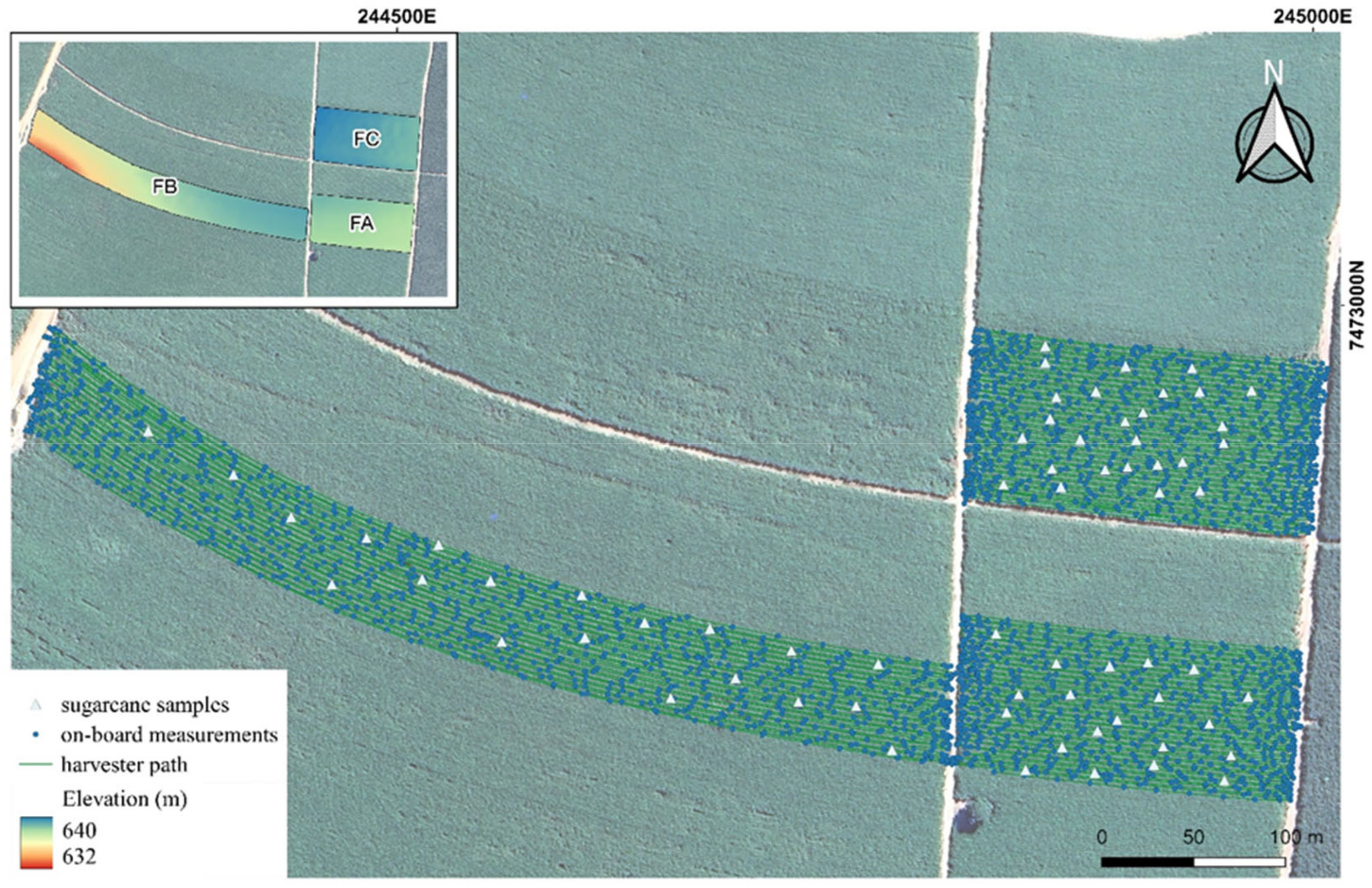
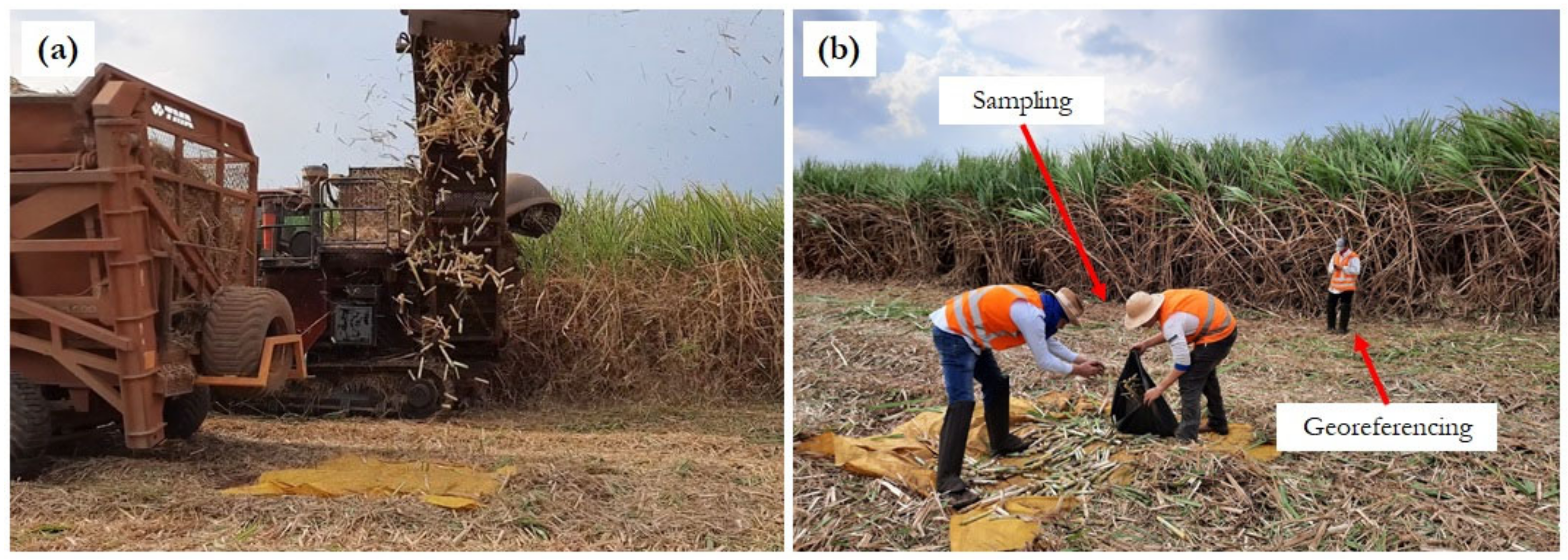
2.2. Field Experiment and Data Acquisition: On-the-Go Measurements

The experiment was performed during three consecutive days of 2020/2021 harvest season in a commercial second ratoon sugarcane field cultivated with CTC 4, with 1.50 m between rows. Although the study area is contiguous, we partitioned the collections into three distinct zones, labeled FA (1.72 ha), FB (3.32 ha), and FC (2.02 ha), respectively (Figure 2).

The NIR software allows on-the-go measurements that involve a calibration step followed by continuous data acquisition. Calibration was performed daily before data acquisition and at noon. The distance of sugarcane billets to the sapphire window decreases the spectrum signal-to-noise ratio due to reduced light intensity. Thus, optimizing spectrometer integration time is essential to mitigate the loss in photometric intensity. A white reference (100% reflectance) was obtained by positioning a 0.40 m² white barium sulfate plate (BaSO₄) beneath the sapphire window in the measurement chamber using halogen lamps [30]. A number of 50 scans and an integration time of 35 ms (0.7 ms per scan), which is equivalent to 1.75 s for each spectral measurement, were set to obtain around 50,000 to 60,000 raw counts of photometric intensity, as recommended by the manufacturer. A dark reference was obtained in the same environment, without the plate and with the lights off.

The spectrometer acquires five to six spectra every 10 s. Anomalies are identified through principal component analysis and Hotteling’s T² test at a 95% confidence level, recording the average non-anomalous spectra. The harvester mean speed was 1 m s⁻¹, and the conveyor belt speed was 2 m s⁻¹, common speed under real conditions [28,29]. Thus, it was necessary to perform an offset for measurement points that was based on the constrained method [31], which uses the sensor batch time (10 s) and the feeding time of the harvester, defined as the time between the entrance of sugarcane in the base cutter and the spectra measurement at the elevator. The feeding time was visually assessed as 10 s, agreeing with other studies and manufacturer information [32]. To determine the offset to the centroid of the harvested line, the distance and time difference between consecutive points were calculated, considering the total measurement time as the sum of feed and batch time. The corrected coordinate was then derived by subtracting the horizontal offset along the track from the initial position.

2.3. Reference Sugarcane Quality Analyses and Spectra Bench Acquisition

Sugarcane samples were randomly collected in the fields during on-board measurements, respecting a minimum of two rows between each collection and performing 20 sugarcane samples for fields FA and FB and 26 for FC. Periodically, the transshipment trailer moved ahead of the harvester, dropping samples onto a canvas on the ground for collection (Figure 3a). Collection points were recorded using a handheld GNSS receiver (Garmin 62 s, accuracy of 5 m, Figure 3b) and further matched with the position of an on-board measured spectra to compose the datasets for data modeling. The billets were packed in plastic bags and sent to the laboratory, where they were stored at 2 °C to minimize the degradation of organic compounds. The next day, fiber, Brix, Pol, Pol of cane, and TRS were assessed following CONSECANA official procedures [6].

Simultaneously with laboratory analysis, bench spectra were obtained for all 66 field samples using the identical NIR sensor employed for on-board measurements. At the laboratory-controlled temperature (20 ± 5 °C), sub-samples of defibrated cane were positioned on a plate to standardize the sample surface. Spectral measurements were made in triplicate at three random points on the surface, storing the average spectrum for each sample.

2.4. Multivariate Data Modeling for Sugarcane Quality Estimation

Two datasets were created: one for field spectra and another for bench spectra, each containing the spectra of 66 samples with their corresponding lab analyses. Descriptive statistics were applied to the sugarcane quality values determined conventionally. The data was partitioned using the Kennard-Stone (KS) algorithm [33] for FA, FB, and FC, comprising 70% for calibration (47 samples, 14 from FA and FB, and 19 from FC), and 30% for validation (19 samples, 6 from FA and FB, and 7 from FC). The KS algorithm was applied to provide 70% of the data from each field designated for calibration, aiming to generate a global calibration model for both fields without bias towards either. The KS algorithm is frequently employed in data modeling to achieve a partition of calibration and validation datasets with equivalent data distribution, which is desirable to test machine learning models.

In the spectral preprocessing step, we applied the standard normal variate (SNV) [34] to all spectra, followed by the second derivative of the Savitzky-Golay algorithm (second SG) [35,36]. SNV was employed to mitigate deviations caused by particle size and scattering, achieving this by centering each spectrum on its mean and scaling it by its standard deviation. To further enhance the signal-to-noise ratio and minimize potential hurdles in the data, the second SG was implemented with a specific window size of nine wavelengths. This window size was determined through a careful selection process, guided by the objective of optimizing the preprocessing procedure. Specifically, the choice of the nine-wavelength window was based on its performance in achieving a lower calibration Root Mean Square Error (RMSE) value, ensuring that the preprocessing parameters were tuned to enhance the overall robustness and accuracy of the subsequent data analysis. The PDS [37] was developed to apply the calibration transfer method in field conditions. This multivariate method aims to extend the accuracy of a master model to new environmental conditions or different instruments [38]. PDS relates wavelengths from a master spectrum (e.g., defibrated sugarcane) to those of a secondary spectrum (e.g., field spectra). Widely used, it effectively calibrates soil spectra from on-board sensing, eliminating noise and humidity effects [15,20,23]. Its main advantages include using a small transfer set and noise-filtering due to its multivariate nature [15]. PDS remains a reference in studies assessing new model transfer methods due to its consistent performance [7].

The bench spectra dataset served as the master spectra, with the field spectra dataset as the secondary spectra for PDS modeling. The algorithm generated a transformation matrix from the master and secondary spectra matrices, allowing calibration model transfer to spectra measured under different conditions. For a complete explanation of PDS modeling, see Wang et al. and Workman [37,39]. The transformation matrix, built with a predefined window (w = 9) using the calibration dataset [23], was applied to the external validation dataset, validating the models. This calibrated model was then extended to all on-board spectra measurements. Principal component analysis (PCA) was conducted for exploratory analysis before and after the calibration transfer application.

The prediction models were developed using partial least squares (PLS) regression and leave-one-out cross-validation [40], as developed by Corrêdo et al. [41]. The PLS regression is often adopted for spectroscopy studies since it can cope with multivariate data, converting it into a new multi-dimensional coordinate system (loadings) through the creation of a smaller number of orthogonal variables (latent variables—LV) [42,43]. The optimal PLS models were determined based on the lowest number of latent variables (LV) and a lower RMSE of the cross-validation value. Both algorithms (PCA and PLS) were based on the NIPALS (Nonlinear Iterative Partial Least Squares) method.

Outliers in the calibration step were identified using Hotelling’s T2 for high leverage and Q statistics for unmodeled residuals. Samples exceeding the 95% significance level for both tests were removed from the spectral dataset. Reference values were assessed by the RMSE of calibration (RMSEC), and samples with prediction errors exceeding ±3 × RMSEC were considered outliers and excluded from the dataset, following the guidelines of ASTM E1655-17 [44]. All modeling was conducted using MATLAB (MATLAB R2015a, The MathWorks Inc., Natick, USA) and PLS-Toolbox 8.8 (Eigenvector Research Inc., Manson, WA, USA).

The models were evaluated in terms of their R², relative root mean square error (RRMSE) in calibration, cross-validation, and external validation, and by the ratio of performance to the interquartile range (RPIQ, Equation (1)).

$$RPIQ=\frac{(Q_3-Q_1)}{RMSE}$$

(1)

where Q₃ and Q₁ are the upper and lower quartiles, respectively. The RPIQ is often used for the evaluation of prediction models based on spectroscopy data because it can better represent the accuracy of predictions in relation to the spread of the population. As pointed out in [45], as RPIQ is not based on standard deviation, it can be a more appropriate metric for measurements without a normal distribution.

The best PDS-PLS models were then applied for the prediction of all on-board spectra acquired. No established method exists for filtering online measurements in spectral prediction models. Outliers in on-board data predicted by PDS-PLS were identified using the average distance to k-nearest neighbors (KNN) in score space. Samples with KNN values exceeding three were considered outliers and removed from the dataset.

2.5. Spatial Variability and Site-Specific Assessment of the Relationships among Sugarcane Quality and Soil Attributes

The spatial prediction used the values predicted by the PDS-PLS models to be interpolated by ordinary kriging (OK). OK requires the adjustment of a semivariogram model for each attribute to be interpolated, obtained through Equation (2):

$$\mathrm{\gamma }\left(\mathbf{h}\right)=\frac{1}{2\mathrm{N}\left(\mathbf{h}\right)}{\sum }_{\mathsf{\alpha }=1}^{\mathrm{N}\left(\mathbf{h}\right)}\left\{\mathrm{Z}\left({\mathbf{x}}_{\mathsf{\alpha }}+\mathbf{h}\right)-\mathrm{z}\left({\mathbf{x}}_{\mathsf{\alpha }}\right)\right\}2$$

(2)

where, γ(h) is the semivariogram for a distance vector (lag) h among the observations z(xα) and Z(xα + h). N(h) was the number of pairs separated by h. Spherical, Exponential, and Gaussian theoretical models were tested for semivariogram adjustment. The model with the lowest cross-validation RMSE was selected [46]. Data were subsequently interpolated into a 1-m grid using global point kriging. Geostatistical analysis and mapping were conducted in QGIS 3.10.8 (QGIS Development Team, 2018).

3. Results and Discussion

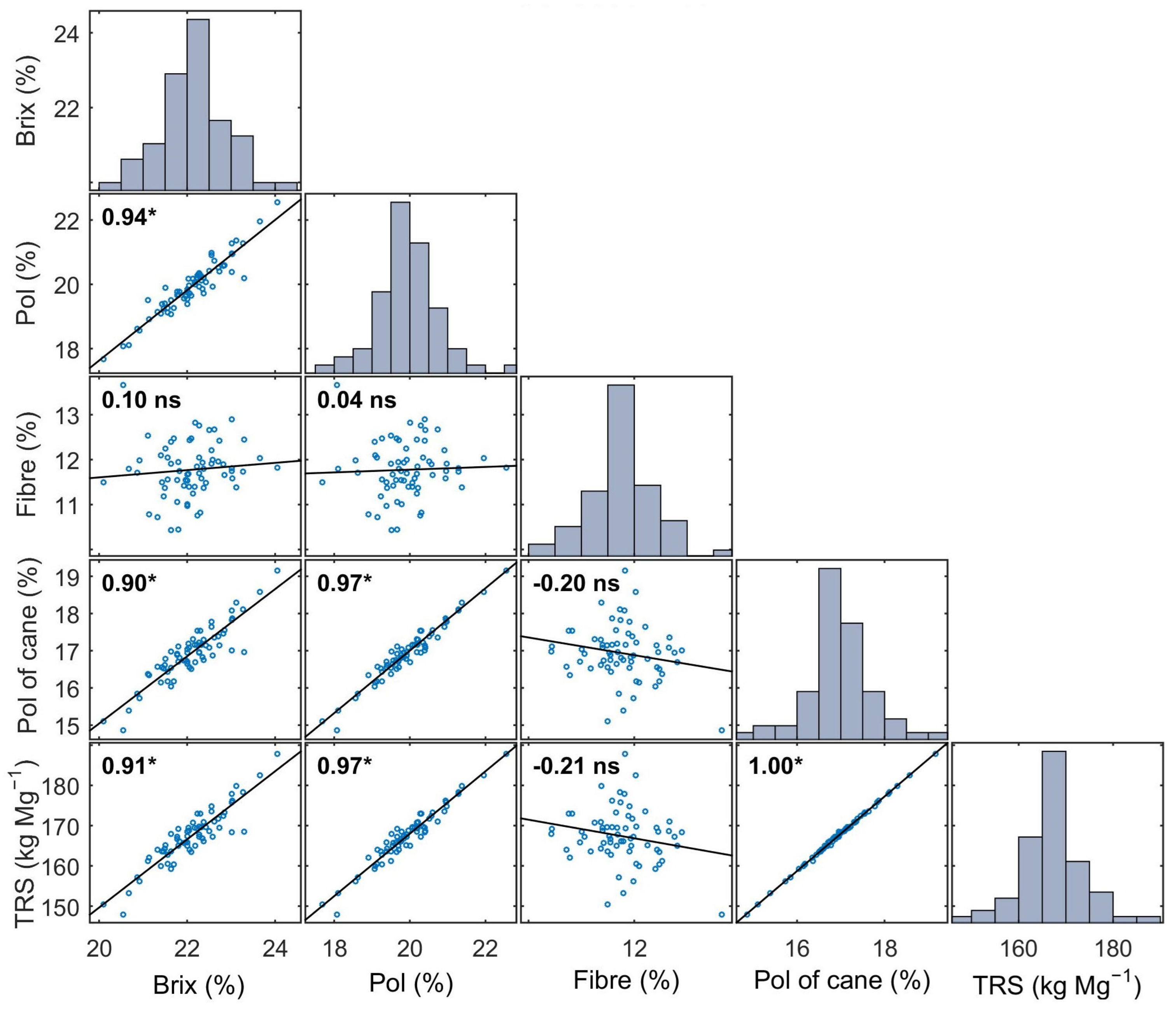
3.1. Sugarcane Quality Properties Characterization

The implementation of the KS algorithm allowed for the creation of a calibration set whose range mirrored that of the complete dataset (

Table 1. Descriptive statistics of the sugarcane quality properties for all collected samples (all data) for the cross-validation (47 samples) and prediction data set (19 samples).

Property	Data Set	Min.	Max.	Mean	S.D.	C.V. (%)	Q1	Q3	Kurt.	Skew.
Brix (%)	All data	20.10	24.05	22.09	0.73	3.30	21.63	22.55	3.43	−0.06
	Cross-val.	20.10	24.05	22.14	0.79	3.57	21.63	22.58	3.34	−0.13
	Pred.	20.92	23.03	21.98	0.57	2.59	21.51	22.37	2.24	−0.09
Pol (%)	All data	17.68	22.55	19.92	0.85	4.27	19.50	20.35	4.15	0.20
	Cross-val.	17.68	22.55	19.93	0.93	4.67	19.50	20.39	3.99	0.21
	Pred.	18.57	20.94	19.88	0.65	3.27	19.40	20.30	2.30	−0.07
Fiber (%)	All data	10.43	13.66	11.77	0.61	5.18	11.42	12.04	3.54	0.22
	Cross-val.	10.43	13.66	11.77	0.62	5.27	11.50	11.99	3.92	0.46
	Pred.	10.44	12.67	11.78	0.60	5.09	11.37	12.25	2.50	−0.45
Pol of cane (%)	All data	14.86	19.16	16.93	0.74	4.37	16.56	17.30	4.41	0.00
	Cross-val.	14.86	19.16	16.95	0.79	4.66	16.57	17.19	4.42	0.03
	Pred.	15.73	17.87	16.90	0.59	3.49	16.37	17.36	2.05	−0.29
	All data	147.84	187.82	167.37	6.82	4.07	163.98	170.77	4.41	−0.05
TRS (kg Mg−1)	Cross-val.	147.84	187.82	167.53	7.32	4.37	164.05	169.67	4.45	−0.03
	Pred.	156.13	176.15	166.98	5.55	3.32	161.25	171.01	2.02	−0.28

Abbreviations: Minimum (Min.); Maximum (Max.); Standard Deviation (S.D.); Coefficient of Variation (C.V.); lower quartile (Q₁); upper quartile (Q₃); Kurtosis (Kurt.); Skewness (Skew.); Cross-val. (cross-validation); Pred. (prediction or external validation); TRS (total recoverable sugars).

). In the complete dataset, variations of approximately 4% for Brix, 4.9% for Pol, 3.2% for fiber, 4.3% for Pol of cane, and 40 kg Mg⁻¹ for TRS were observed. The coefficients of variation (CV) for all sugarcane quality attributes exhibited a range of 3 to 5%, both in the calibration by cross-validation and prediction datasets. The interquartile range revealed discrepancies below 1% for Brix, Pol, fiber, and Pol of cane, while TRS manifested variations between 5.62 and 9.76 kg Mg⁻¹ for cross-validation and prediction datasets.

Positive skewness was evident in Pol and fiber, whereas Brix, Pol of cane, and TRS approached zero skewness. Positive kurtosis across all variables signified a concentration of values around the mean and median, with distribution curves showing no flattening. Most sugarcane quality attributes demonstrated significant (p < 0.05) Pearson’s correlations surpassing 0.90, except for fiber, which exhibited non-significant correlations (Figure A1 in the Appendix A). This is expected since all this quality variables are related to sucrose content, and other soluble solids, such as reducing sugars and non-sugars, account for less than 2% of the total physicochemical constitution of sugarcane [41,47].

Characterizing the three fields evaluated, Field C (FC, Figure 4) showed lower absolute mean values for all sugarcane quality properties than fields A and B (FA and FB, respectively). On the other hand, these values were higher for field B (FB) than the other fields. The smallest interquartile distance was observed for field B, especially for Pol of cane and TRS.

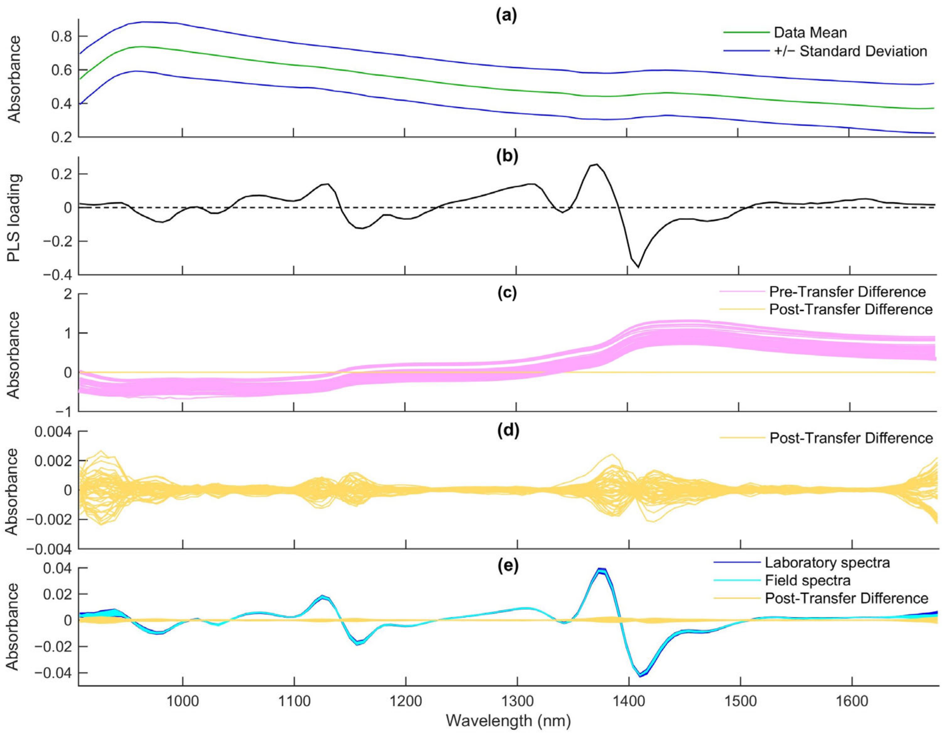
3.2. Processing of Spectral Data

The first LV for each of the five considered sugarcane quality attributes accounted for a great part of the variance within each population—99.30% for fiber, 96.67% for Brix, 94.43% for Pol, 87.82% for TRS, and 87.49% for Pol of cane. Despite variations in the explained variance percentages, all variables exhibited similar plots for the first loading (Figure 5a). The smallest variation, primarily attributed to saccharides and the third overtone of O-H, occurred between 900 and 1000 nm and is typically associated with cellulosic fiber [48]. Around 960 nm, a corresponding effect of the third overtone of C-H stretching, possibly related to polysaccharides such as sucrose, was observed [49]. An intermediate variation is evident between 1100 and 1200 nm, where the second vibrational frequency overtones associated with C-H stretching and sugars were identified [49]. Additionally, spectral bands around 1170–1180 nm, linked to the third overtone of C-H and unsaturated C=C double bonds, typically associated with fiber, such as lignin, were noted [48]. The most significant variation within the wavelength range of the equipment used in this study was between 1300 and 1450 nm, stabilizing close to zero explained variance by the first latent variable after this interval. Effects possibly related to C-H combinations and the O-H first overtone were observed at 1360 nm [50]. Bands associated with sugars, including C-H and O-H related bands, were identified around 1450 nm, represented by the second overtone of O-H and polysaccharides linked to O-H [48].

The spectra acquired through on-board sensing showed substantial differences from those obtained under bench conditions (Figure 5b), as expected [3,27]. For both defibrated and on-board datasets, spectra preprocessing and the PDS method allowed substantial mitigation of these differences (Figure 5c). Although the PDS allowed the spectra obtained by on-board sensing to exhibit very similar morphology to the spectra obtained on the bench, it still maintains slight differences, primarily in the bands corresponding to the absorbance peaks with the highest data variance (Figure 5d).

The PCA of the spectra of the measurements taken on board before and after the calibration transfer confirms a certain robustness of the PDS applied to the spectral data, which substantially reduced the variance due to measurement differences between the bench and on-board data sets (Figure 6). The scores of the laboratory spectra are divided into two clear groups (Figure 6a), in which a variance of 93.56% is explained by the first two components. After applying the PDS model, both spectra are represented in the space of the main data set, with the confidence interval of the field data contained in that of the data collected on the bench (Figure 6b). The first two components explained 85.05% of the variance in the data after the PDS calibration transfer. The variation in data obtained from on-board measurements may be due mainly to adverse environmental factors intrinsic to mechanized harvesting (e.g., variation in external brightness, presence of impurities and dirt, vibrations, and surface irregularities of the measured samples). The calibration transfer method for noise correction of spectral data collection on board the harvester was reasonably successful, despite not being able to fully correct for environmental effects related to harvesting.

3.3. Sugarcane Quality Properties Prediction Models

All PLS prediction models used seven LVs, except fiber’s, which used only four. Fiber also presented the lowest R² and highest RRMSE values, with R² of 0.18 and RRMSE% of 3.97 for on-board measurements and R² of 0.13 and RRMSE% of 4.16 for laboratory measurements. The best performance was observed for Brix prediction (Figure 7). The comparison between the prediction using laboratory-measured and on-board spectra demonstrates the effectiveness of the PDS for on-board spectra acquisition during sugarcane harvest. The RRMSE for Pol showed consistent values in both laboratory and on-board measurements (2.51%). Pol of cane was closely matched, at 2.75% in the lab and 2.73% on-board. Similar trends were observed for Brix and TRS, with values of 1.86% and 2.75%, and 1.59% and 2.56%, for on-board and laboratory measurements, respectively. RPIQ values were also comparable. The Pol and Pol of the cane were comparable for on-board (2.10 and 2.14) and laboratory measurements (1.81 and 2.13). Brix and TRS were slightly higher in lab measurements (2.46 and 2.28) than on-board measurements (2.10 and 2.12). Fiber predictive performance was marginally higher for online measurements (1.88) than for laboratory measurements (1.79).

Comparing with other studies, Nawi et al. [25] achieved a Brix prediction RMSEP of 1.51% (relative accuracy: 8.47%) using NIR absorbance spectra from the outer surface under controlled conditions. In cross-section measurements of billet samples under control, Nawi et al. [26] achieved RRMSEP values up to 8.13% (RMSEP = 1.45%) for Brix prediction. Phuphaphud et al. [51] obtained fiber prediction results of up to 5.49% (RMSEP = 0.63%) directly from the outer surface of sugarcane stalks’ peel. In a study on waxy material and measurement position’s effect on Pol prediction, Maraphum et al. [52] achieved relative accuracy results of up to 6.25% (RRMSEP = 1.20%). The prediction performance in this study, possibly due to the calibration transfer procedure, was comparable to or higher than previously reported results.

Before our study, NIR spectroscopy for on-board Brix sensing was only tested in controlled conditions using sugarcane harvester elevator replicas. Udompetaikul et al. [29] found that sugarcane delivery levels in the elevator influenced prediction performance. Despite the best results in a full delivery elevator, they calibrated a model for uneven cane levels, achieving R² of 0.56 and RRMSEP of 1.86% and 1.83%, respectively. Our study replicated this in field conditions, showing a 1.86% relative accuracy for the same quality attribute, consistent with controlled conditions.

3.4. On-Board Data Analysis and Spatial Variability

Geostatistical analysis showed that sugarcane quality parameters were spatially dependent across the field (

Table 2. Semivariogram model parameters of sugarcane quality properties used for mapping the spatial variability for the three experimental fields.

Field	Property	Model Fit	C0	C0 + C1	A (m)	C0/(C0 + C1)
FA	Brix (%)	Exponential	0.060	0.098	33.62	0.61
	Pol (%)	Spherical	0.091	0.223	71.53	0.41
	Fiber (%)	Gaussian	0.036	0.043	92.93	0.84
	Pol of cane (%)	Spherical	0.071	0.161	75.74	0.44
	TRS (kg Mg−1)	Spherical	6.250	13.019	73.78	0.48
FB	Brix (%)	Exponential	0.252	0.363	64.48	0.69
	Pol (%)	Spherical	0.349	0.444	62.98	0.79
	Fiber (%)	Spherical	0.108	0.117	264.23	0.92
	Pol of cane (%)	Spherical	0.293	0.360	66.12	0.81
	TRS (kg Mg−1)	Spherical	25.176	31.016	66.01	0.81
FC	Brix (%)	Exponential	0.381	0.517	38.76	0.74
	Pol (%)	Exponential	0.500	0.629	58.34	0.79
	Fiber (%)	Spherical	0.136	0.212	118.73	0.64
	Pol of cane (%)	Spherical	0.396	0.508	93.10	0.78
	TRS (kg Mg−1)	Spherical	34.424	44.395	97.67	0.78

Header abbreviations: nugget variance (C₀); spatial dependent variance (C₁); range (A); nugget-to-sill [C₀/(C₀ + C₁)]; total recoverable sugars (TRS).

). However, the nugget variance (C₀) represents a considerable portion of the sill variance (C₀ + C₁), implying that portion is not spatially related. Accordingly, the space dependence index (SDI) proposed by Cambardella et al. [53] show that Brix is moderately spatially dependent in the three fields. In FA, all sugarcane quality properties showed moderate spatial dependence, except fiber, which showed weak spatial dependence. In FB, all quality properties except Brix were weakly spatially dependent. In FC, besides Brix, Pol was moderately spatially dependent, and the other properties were weakly spatially dependent. Rodrigues et al. [54] fitted variograms to predict Brix, Pol, and fiber from physical-chemical soil parameters and leaf nitrogen as predictor variables. The results corroborated the present study, showing weakly to moderately spatial dependence of all quality parameters evaluated, except for fiber, with strongly spatial dependence on the second harvest season.

Despite inherent measurement errors tied to technique limitations in mechanized harvesting, including variable sensor-target distance and environmental challenges, a discernible spatial structure is evident in variograms even within the small areas tested (1.7 to 3.3 ha). The range of sugarcane quality properties spanned approximately 33–264 m, with sugar concentration parameters (Brix, Pol, Pol of cane, and TRS) having a maximum range of 98 m. Notably, there was variability at short distances, particularly for Brix (range: 34 to 65 m), indicating diverse quality content regions in the fields. This aligns with findings by Johnson and Richard [55], who reported a spatial correlation for yield and sugarcane quality parameters in Louisiana (USA) with ranges from 26 to 133 m. Catelan et al. [56] also identified strong spatial dependence in Brix, Pol, fiber, TRS, and sugarcane yield in a 445 ha area with a low sample density collected manually.

Sugarcane quality maps revealed significant variability across the experimental fields (Figure 8), with pronounced distinctions among the fields themselves. Notably, Field C exhibited a larger area with lower concentrations of all quality parameters compared to Fields A and B, as depicted in Figure 4. Laboratory measurements for calibration and validation of prediction models affirm this trend, indicating lower quality parameter contents in Field C compared to Fields A and B. The modeling effectively discriminates between high and low values of sugarcane quality properties, showcasing this distinction even within small areas and over substantial distances.

Brix, Pol, fiber, and Pol of cane had range variations of 7.14%, 8.91%, 7.63%, and 9.27%, respectively. The range of TRS was 8.62%, representing 14 kg Mg⁻¹. The combined use of this parameter with yield data may enable real-time maps of sugar produced per area. It constitutes valuable information not only for the agronomic management aiming at the quality of the product supplied to the mills but also for the industrial operation planning and financial management of the entire operation between sugar mills and suppliers.

Achieving comparable predictive performance to methods of controlled conditions in NIR spectroscopy is challenging due to factors such as sample surface uniformity and external interferences [7]. This study confirmed the potential of the PDS calibration transfer method to overcome some intrinsic adversities of mechanized sugarcane harvesting. In real-world field conditions, the control of cane levels in the elevator may make the implementation of an on-board system unfeasible. Therefore, it is necessary to explore diverse methods of post-processing spectra combined with the optimization of sensor system parameters (e.g., sensor-target distance and electromagnetic radiation intensity). The combination of NIR instrumentation and PDS application was crucial to the technique’s performance in a real sugarcane harvest system. We integrated harvester elevator acquisition, previously tested only under controlled conditions [28,29], with spectra from sugarcane billets.

Despite the additional challenge presented by the narrow range of quality parameter values [28], as observed in the small nearby fields of this study, the technique allowed the identification of variability within the field. It demonstrated a prediction error comparable to that of other studies, suggesting its potential utility for industry control and agronomic decision-making. Furthermore, the goals of spatialized estimates in precision agriculture are both qualitative and quantitative. In a study like this, the technology is expected to enable mapping regions with tendencies toward lower or higher quality for localized management. The high-density information collection would compensate for sensor accuracy [3], as the data undergoes geostatistical analysis and interpolation. In summary, the mere ability to capture variations in quality attributes in the field represents an advancement in spatial management using precision agriculture techniques.

Future studies should extend this methodology to evaluate extensive commercial fields across multiple harvest seasons and at various moments within the season, facilitating clearer identification of spatial patterns for sugarcane quality parameters. Yield data can be integrated to analyze relationships between quantity and quality parameters. Acquiring such a comprehensive database will enable the development of more robust calibration models with greater variability in quality properties, leveraging the technique on a commercial scale.

Different external illumination sets and sensing distances can be tested to minimize the obstruction of the sapphire window by dirt. Exploring higher frequencies of data collection and employing unsupervised data processing techniques can further optimize transfer-related parameters. Additionally, improving model results can be pursued by combining more advanced variable combination and calibration transfer methods based on NIR data already collected at high density by the industry’s quality laboratory throughout the harvest. The implementation of this sensor in harvester fleets is dependent on acquisition costs, necessitating the development of system simplifications. The selection of spectral variables, a well-established chemometrics technique, can assist in this task.

4. Conclusions

This study has shown that it is possible to overcome the partially adverse effects of on-board sensing on sugarcane harvesters and provide spatial data on crop quality. Piecewise direct standardization allowed transferring NIR calibration models developed by partial least squares regression on the bench from defibrated cane samples to perform post-processing of data obtained by the on-board sensor in the harvester. Furthermore, the on-board sensor and the proposed method for prediction allowed the spatial variability of sugarcane quality attributes to be characterized. The results were consistent with previous studies, which strengthens the conclusion about the effectiveness of the proposed method for onboard proximal sensing of sugarcane quality to map the spatial variability of technological quality parameters.

References

1. Molin, J.P.; Bazame, H.C.; Maldaner, L.; Corredo, L.D.P.; Martello, M.; Canata, T.F.; de Paula Corredo, L.; Martello, M.; Canata, T.F. Precision Agriculture and the Digital Contributions for Site-Specific Management of the Fields. Rev. Ciência Agronômica 2020, 51, 1–10. [Google Scholar] [CrossRef]
2. Cortés, V.; Blasco, J.; Aleixos, N.; Cubero, S.; Talens, P. Monitoring Strategies for Quality Control of Agricultural Products Using Visible and Near-Infrared Spectroscopy: A Review. Trends Food Sci. Technol. 2019, 85, 138–148. [Google Scholar] [CrossRef]
3. Corrêdo, L.d.P.; Canata, T.F.; Maldaner, L.F.; de Lima, J.d.J.A.; Molin, J.P. Sugarcane Harvester for In-Field Data Collection: State of the Art, Its Applicability and Future Perspectives. Sugar Tech. 2020, 22, 1–14. [Google Scholar] [CrossRef]
4. Bramley, R.G.V. Lessons from Nearly 20 Years of Precision Agriculture Research, Development, and Adoption as a Guide to Its Appropriate Application. Crop Pasture Sci. 2009, 60, 197–217. [Google Scholar] [CrossRef]
5. Maldaner, L.F.; Corrêdo, L.d.P.; Canata, T.F.; Molin, J.P. Predicting the Sugarcane Yield in Real-Time by Harvester Engine Parameters and Machine Learning Approaches. Comput. Electron. Agric. 2021, 181, 105945. [Google Scholar] [CrossRef]
6. CONSECANA. Sugarcane, Sugar, and Alcohol Producers Council of the State of São Paulo, Instruction Manual, 5th ed.; CONSECANA: Piracicaba, SP, Brazil; Consecana, SP, Brazil, 2006. [Google Scholar]
7. Pasquini, C. Near Infrared Spectroscopy: A Mature Analytical Technique with New Perspectives—A Review. Anal. Chim. Acta 2018, 1026, 8–36. [Google Scholar] [CrossRef] [PubMed]
8. Walsh, K.B.; Blasco, J.; Zude-Sasse, M.; Sun, X. Visible-NIR ‘Point’ Spectroscopy in Postharvest Fruit and Vegetable Assessment: The Science behind Three Decades of Commercial Use. Postharvest Biol. Technol. 2020, 168, 111246. [Google Scholar] [CrossRef]
9. Sexton, J.; Everingham, Y.; Donald, D.; Staunton, S.; White, R. Investigating the Identification of Atypical Sugarcane Using NIR Analysis of Online Mill Data. Comput. Electron. Agric. 2020, 168, 105111. [Google Scholar] [CrossRef]
10. Ruangratanakorn, J.; Suwonsichon, T.; Kasemsumran, S.; Thanapase, W. Installation Design of On-Line near Infrared Spectroscopy for the Production of Compound Fertilizer. Vib. Spectrosc. 2020, 106, 103008. [Google Scholar] [CrossRef]
11. Xu, X.; Mo, J.; Xie, L.; Ying, Y. Influences of Detection Position and Double Detection Regions on Determining Soluble Solids Content (SSC) for Apples Using On-Line Visible/Near-Infrared (Vis/NIR) Spectroscopy. Food Anal. Methods 2019, 12, 2078–2085. [Google Scholar] [CrossRef]
12. Salguero-Chaparro, L.; Peña-Rodríguez, F. On-Line versus off-Line NIRS Analysis of Intact Olives. LWT—Food Sci. Technol. 2014, 56, 363–369. [Google Scholar] [CrossRef]
13. Porep, J.U.; Kammerer, D.R.; Carle, R. On-Line Application of near Infrared (NIR) Spectroscopy in Food Production. Trends Food Sci. Technol. 2015, 46, 211–230. [Google Scholar] [CrossRef]
14. Munnaf, M.A.; Mouazen, A.M. Development of a Soil Fertility Index Using On-Line Vis-NIR Spectroscopy. Comput. Electron. Agric. 2021, 188, 106341. [Google Scholar] [CrossRef]
15. Nawar, S.; Munnaf, M.A.; Mouazen, A.M. Machine Learning Based On-Line Prediction of Soil Organic Carbon after Removal of Soil Moisture Effect. Remote Sens. 2020, 12, 1308. [Google Scholar] [CrossRef]
16. Tümsavaş, Z.; Tekin, Y.; Ulusoy, Y.; Mouazen, A.M. Prediction and Mapping of Soil Clay and Sand Contents Using Visible and Near-Infrared Spectroscopy. Biosyst. Eng. 2019, 177, 90–100. [Google Scholar] [CrossRef]
17. Long, D.S.; McCallum, J.D. Adapting a Relatively Low-Cost Reflectance Spectrometer for on-Combine Sensing of Grain Protein Concentration. Comput. Electron. Agric. 2020, 174, 105467. [Google Scholar] [CrossRef]
18. Yang, S.; Wu, Q.; Chang, H.; Li, Q.; Xu, H. Effect of Grain Density to near Infrared Spectra and Design of a Laboratory Evaluation System for Combine Harvester. In Proceedings of the 2017 ASABE Annual International Meeting, Spokane, WA, USA, 16–19 July 2017; pp. 1–8. [Google Scholar] [CrossRef]
19. Risius, H.; Hahn, J.; Huth, M.; Tölle, R.; Korte, H. In-Line Estimation of Falling Number Using near-Infrared Diffuse Reflectance Spectroscopy on a Combine Harvester. Precis. Agric. 2015, 16, 261–274. [Google Scholar] [CrossRef]
20. Franceschini, M.H.D.; Demattê, J.A.M.; Kooistra, L.; Bartholomeus, H.; Rizzo, R.; Fongaro, C.T.; Molin, J.P. Effects of External Factors on Soil Reflectance Measured On-the-Go and Assessment of Potential Spectral Correction through Orthogonalisation and Standardisation Procedures. Soil. Tillage Res. 2018, 177, 19–36. [Google Scholar] [CrossRef]
21. Kuang, B.; Tekin, Y.; Mouazen, A.M. Comparison between Artificial Neural Network and Partial Least Squares for On-Line Visible and near Infrared Spectroscopy Measurement of Soil Organic Carbon, PH and Clay Content. Soil. Tillage Res. 2015, 146, 243–252. [Google Scholar] [CrossRef]
22. Morellos, A.; Pantazi, X.E.; Moshou, D.; Alexandridis, T.; Whetton, R.; Tziotzios, G.; Wiebensohn, J.; Bill, R.; Mouazen, A.M. Machine Learning Based Prediction of Soil Total Nitrogen, Organic Carbon and Moisture Content by Using VIS-NIR Spectroscopy. Biosyst. Eng. 2016, 152, 104–116. [Google Scholar] [CrossRef]
23. Ji, W.; Viscarra Rossel, R.A.; Shi, Z. Improved Estimates of Organic Carbon Using Proximally Sensed Vis-NIR Spectra Corrected by Piecewise Direct Standardization. Eur. J. Soil. Sci. 2015, 66, 670–678. [Google Scholar] [CrossRef]
24. Ji, W.; Viscarra Rossel, R.A.; Shi, Z. Accounting for the Effects of Water and the Environment on Proximally Sensed Vis-NIR Soil Spectra and Their Calibrations. Eur. J. Soil. Sci. 2015, 66, 555–565. [Google Scholar] [CrossRef]
25. Nawi, N.M.; Chen, G.; Jensen, T.; Mehdizadeh, S.A. Prediction and Classification of Sugar Content of Sugarcane Based on Skin Scanning Using Visible and Shortwave near Infrared. Biosyst. Eng. 2013, 115, 154–161. [Google Scholar] [CrossRef]
26. Nawi, N.M.; Chen, G.; Jensen, T. Visible and Shortwave near Infrared Spectroscopy for Predicting Sugar Content of Sugarcane Based on a Cross-Sectional Scanning Method. J. Near Infrared Spectrosc. 2013, 21, 289–297. [Google Scholar] [CrossRef]
27. Nawi, N.M.; Chen, G.; Jensen, T. In-Field Measurement and Sampling Technologies for Monitoring Quality in the Sugarcane Industry: A Review. Precis. Agric. 2014, 15, 684–703. [Google Scholar] [CrossRef]
28. Phetpan, K.; Udompetaikul, V.; Sirisomboon, P. An Online Visible and Near-Infrared Spectroscopic Technique for the Real-Time Evaluation of the Soluble Solids Content of Sugarcane Billets on an Elevator Conveyor. Comput. Electron. Agric. 2018, 154, 460–466. [Google Scholar] [CrossRef]
29. Udompetaikul, V.; Phetpan, K.; Sirisomboon, P. Development of the Partial Least-Squares Model to Determine the Soluble Solids Content of Sugarcane Billets on an Elevator Conveyor. Measurement 2021, 167, 107898. [Google Scholar] [CrossRef]
30. Mayrink, G.O.; Valente, D.S.M.; Queiroz, D.M.; Pinto, F.A.C.; Teofilo, R.F. Determination of Chemical Soil Properties Using Diffuse Reflectance and Ion-Exchange Resins. Precis. Agric. 2019, 20, 541–561. [Google Scholar] [CrossRef]
31. Delefortrie, S.; Saey, T.; De Pue, J.; Van De Vijver, E.; De Smedt, P.; Van Meirvenne, M. Evaluating Corrections for a Horizontal Offset between Sensor and Position Data for Surveys on Land. Precis. Agric. 2016, 17, 349–364. [Google Scholar] [CrossRef]
32. Magalhães, P.S.G.; Cerri, D.G.P. Yield Monitoring of Sugar Cane. Biosyst. Eng. 2007, 96, 1–6. [Google Scholar] [CrossRef]
33. Kennard, R.W.; Stone, L.A. Computer Aided Design of Experiments. Technometrics 1969, 11, 137–148. [Google Scholar] [CrossRef]
34. Barnes, R.J.; Dhanoa, M.S.; Lister, S.J. Standard Normal Variate Transformation and De-Trending of near-Infrared Diffuse Reflectance Spectra. Appl. Spectrosc. 1989, 43, 772–777. [Google Scholar] [CrossRef]
35. Savitzky, A.; Golay, M.J.E. Smoothing and Differentiation of Data by Simplified Least Squares Procedures. Anal. Chem. 1964, 36, 1627–1639. [Google Scholar] [CrossRef]
36. Oliveri, P.; Malegori, C.; Simonetti, R.; Casale, M. The Impact of Signal Pre-Processing on the Final Interpretation of Analytical Outcomes—A Tutorial. Anal. Chim. Acta 2019, 1058, 9–17. [Google Scholar] [CrossRef] [PubMed]
37. Wang, Y.; Veltkamp, D.J.; Kowalski, B.R. Multivariate Instrument Standardization. Anal. Chem. 1991, 63, 2750–2756. [Google Scholar] [CrossRef]
38. Feudale, R.N.; Woody, N.A.; Tan, H.; Myles, A.J.; Brown, S.D.; Ferré, J. Transfer of Multivariate Calibration Models: A Review. Chemom. Intell. Lab. Syst. 2002, 64, 181–192. [Google Scholar] [CrossRef]
39. Workman, J.J. A Review of Calibration Transfer Practices and Instrument Differences in Spectroscopy. Appl. Spectrosc. 2018, 72, 340–365. [Google Scholar] [CrossRef]
40. Wold, S.; Martens, H.; Wold, H. The Multivariate Calibration Problem in Chemistry Solved by the PLS Method. In Matrix Pencils; Springer: Berlin/Heidelberg, Germany, 1983; pp. 286–293. [Google Scholar]
41. Corrêdo, L.d.P.; Maldaner, L.F.; Bazame, H.C.; Molin, J.P. Evaluation of Minimum Preparation Sampling Strategies for Sugarcane Quality Prediction by Vis-Nir Spectroscopy. Sensors 2021, 21, 2195. [Google Scholar] [CrossRef]
42. Pomares-Viciana, T.; Martínez-Valdivieso, D.; Font, R.; Gómez, P.; del Río-Celestino, M. Characterisation and Prediction of Carbohydrate Content in Zucchini Fruit Using near Infrared Spectroscopy. J. Sci. Food Agric. 2018, 98, 1703–1711. [Google Scholar] [CrossRef]
43. Wold, S.; Sjöström, M.; Eriksson, L. PLS-Regression: A Basic Tool of Chemometrics. Chemom. Intell. Lab. Syst. 2001, 58, 109–130. [Google Scholar] [CrossRef]
44. 44. ASTM E1655-17; Standard Practices for Infrared Multivariate Quantitative Analysis. ASTM International: West Conshohocken, PA, USA, 2017; Volume 05.
45. Bellon-Maurel, V.; Fernandez-Ahumada, E.; Palagos, B.; Roger, J.M.; McBratney, A. Critical Review of Chemometric Indicators Commonly Used for Assessing the Quality of the Prediction of Soil Attributes by NIR Spectroscopy. TrAC—Trends Anal. Chem. 2010, 29, 1073–1081. [Google Scholar] [CrossRef]
46. Maldaner, L.F.; Molin, J.P. Data Processing within Rows for Sugarcane Yield Mapping. Sci. Agric. 2020, 77, e20180391. [Google Scholar] [CrossRef]
47. Da Costa, M.V.A.; Fontes, C.H.; Carvalho, G.; Júnior, E.C.d.M. UltraBrix: A Device for Measuring the Soluble Solids Content in Sugarcane. Sustainability 2021, 13, 1227. [Google Scholar] [CrossRef]
48. Workman, J., Jr.; Weyer, L. Practical Guide and Spectral Atlas for Interpretive Near-Infrared Spectroscopy; Routledge: London, UK, 2012; ISBN 9781439875261. [Google Scholar]
49. Golic, M.; Walsh, K.; Lawson, P. Short-Wavelength near-Infrared Spectra of Sucrose, Glucose, and Fructose with Respect to Sugar Concentration and Temperature. Appl. Spectrosc. 2003, 57, 139–145. [Google Scholar] [CrossRef]
50. Osborne, B.G. Near-Infrared Spectroscopy in Food Analysis. Encycl. Anal. Chem. 2006, 14. [Google Scholar] [CrossRef]
51. Phuphaphud, A.; Saengprachatanarug, K.; Posom, J.; Maraphum, K.; Taira, E. Prediction of the Fibre Content of Sugarcane Stalk by Direct Scanning Using Visible-Shortwave near Infrared Spectroscopy. Vib. Spectrosc. 2019, 101, 71–80. [Google Scholar] [CrossRef]
52. Maraphum, K.; Chuan-Udom, S.; Saengprachatanarug, K.; Wongpichet, S.; Posom, J.; Phuphaphud, A.; Taira, E. Effect of Waxy Material and Measurement Position of a Sugarcane Stalk on the Rapid Determination of Pol Value Using a Portable near Infrared Instrument. J. Near Infrared Spectrosc. 2018, 26, 287–296. [Google Scholar] [CrossRef]
53. Cambardella, C.A.; Moorman, T.B.; Novak, J.M.; Parkin, T.B.; Karlen, D.L.; Turco, R.F.; Konopka, A.E. Field-Scale Variability of Soil Properties in Central Iowa Soils. Soil. Sci. Soc. Am. J. 1994, 58, 1501–1511. [Google Scholar] [CrossRef]
54. Rodrigues, F.A.; Magalhães, P.S.G.; Franco, H.C.J. Soil Attributes and Leaf Nitrogen Estimating Sugar Cane Quality Parameters: Brix, Pol and Fibre. Precis. Agric. 2013, 14, 270–289. [Google Scholar] [CrossRef]
55. Johnson, R.M.; Richard, E.P. Sugarcane Yield, Sugarcane Quality, and Soil Variability in Louisiana. Agron. J. 2005, 97, 760–771. [Google Scholar] [CrossRef]
56. Catelan, M.G.; Marques Júnior, J.; Siqueira, D.S.; Gomes, R.P.; Bahia, A.S.R.d.S. Sugarcane Yield and Quality Using Soil Magnetic Susceptibility. Sci. Agric. 2022, 79. [Google Scholar] [CrossRef]
Figure 1. MicroNIR spectrometer (a); device bottom view (b); instrumentation of sensors and radiation sources on the measurement platform on-board of the harvester elevator (c); detail of the measurement chamber position and GNSS receiver in the sugarcane harvester (d).
Agriengineering 06 00005 g001
Figure 2. Location of experimental fields (Fields A, B, and C, respectively FA, FB, and FC), on-board measurement points during harvest, and sampling points for sugarcane and soil. The relief conditions are shown in detail.
Agriengineering 06 00005 g002
Figure 3. Sample collection procedure for modeling and validation. Sugarcane billet samples being dumped on a canvas on the ground (a); georeferencing sample collection (b).
Agriengineering 06 00005 g003
Figure 4. Boxplots of laboratory results for each quality property for all 66 samples collected from the three fields (All), and for the individual fields A, B, and C (FA, FB, and FC).
Agriengineering 06 00005 g004
Figure 5. Mean and standard deviation of spectral data collected in real-time on the harvester (a). First Partial Least Square loading sugarcane quality properties using near-infrared reflectance spectroscopy (b). Spectra difference pre- and post-calibration transfer application (c). Detail of post-transfer difference between spectra data (d). Differences among spectra of sugarcane billet samples with on-board readings by the NIR sensor during the harvest and after processing in the form of defibrated cane with bench readings before and after calibration transfer by Picewise Direct Standardization (PDS) (e).
Agriengineering 06 00005 g005
Figure 6. The principal component scores for on-board field prediction and defibrated cane samples measured in the laboratory before (a) and after (b) calibration transfer by Piecewise Direct Standardization (PDS). The percentage of variance explained by each component is shown on the axes in parentheses.
Agriengineering 06 00005 g006
Figure 7. Predicted values by PLS-PDS models (on-board measurements) versus measured values by conventional laboratory methods (lab measurements) for sugarcane quality properties. TRS: total recoverable sugars.
Agriengineering 06 00005 g007
Figure 8. Sugarcane quality spatial variability maps for the three experimental fields measured by the on-board NIR sensor on the harvester and predicted by PLS regression models combined with the piecewise direct standardization calibration transfer method.
Agriengineering 06 00005 g008