Visual Detection of Portunus Survival Based on YOLOV5 and RCN Multi-Parameter Fusion

Abstract

Single-frame circulation aquaculture belongs to the important category of sustainable agriculture development. In light of the visual-detection problem related to survival rate of Portunus in single-frame three-dimensional aquaculture, a fusion recognition algorithm based on YOLOV5, RCN (RefineContourNet) image recognition of residual bait ratio, centroid moving distance, and rotation angle was put forward. Based on three-parameter identification and LWLR (Local Weighted Linear Regression), the survival rate model of each parameter of Portunus was established, respectively. Then, the softmax algorithm was used to obtain the classification and judgment fusion model of Portunus’ survival rate. In recognition of the YOLOV5 residual bait and Portunus centroid, the EIOU (Efficient IOU) loss function was used to improve the recognition accuracy of residual bait in target detection. In RCN, Portunus edge detection and recognition, the optimized binary cross-entropy loss function based on double thresholds successfully improved the edge clarity of the Portunus contour. The results showed that after optimization, the mAP (mean Average Precision) of YOLOV5 was improved, while the precision and mAP (threshold 0.5:0.95:0.05) of recognition between the residual bait and Portunus centroid were improved by 2% and 1.8%, respectively. The loss of the optimized RCN training set was reduced by 4%, and the rotation angle of Portunus was obtained using contour. The experiment shows that the recognition accuracy of the survival rate model was 0.920, 0.840, and 0.955 under the single parameters of centroid moving distance, residual bait ratio, and rotation angle, respectively; and the recognition accuracy of the survival rate model after multi-feature parameter fusion was 0.960. The accuracy of multi-parameter fusion was 5.5% higher than that of single-parameter (average accuracy). The fusion of multi-parameter relative to the single-parameter (average) accuracy was a higher percentage.

1. Introduction

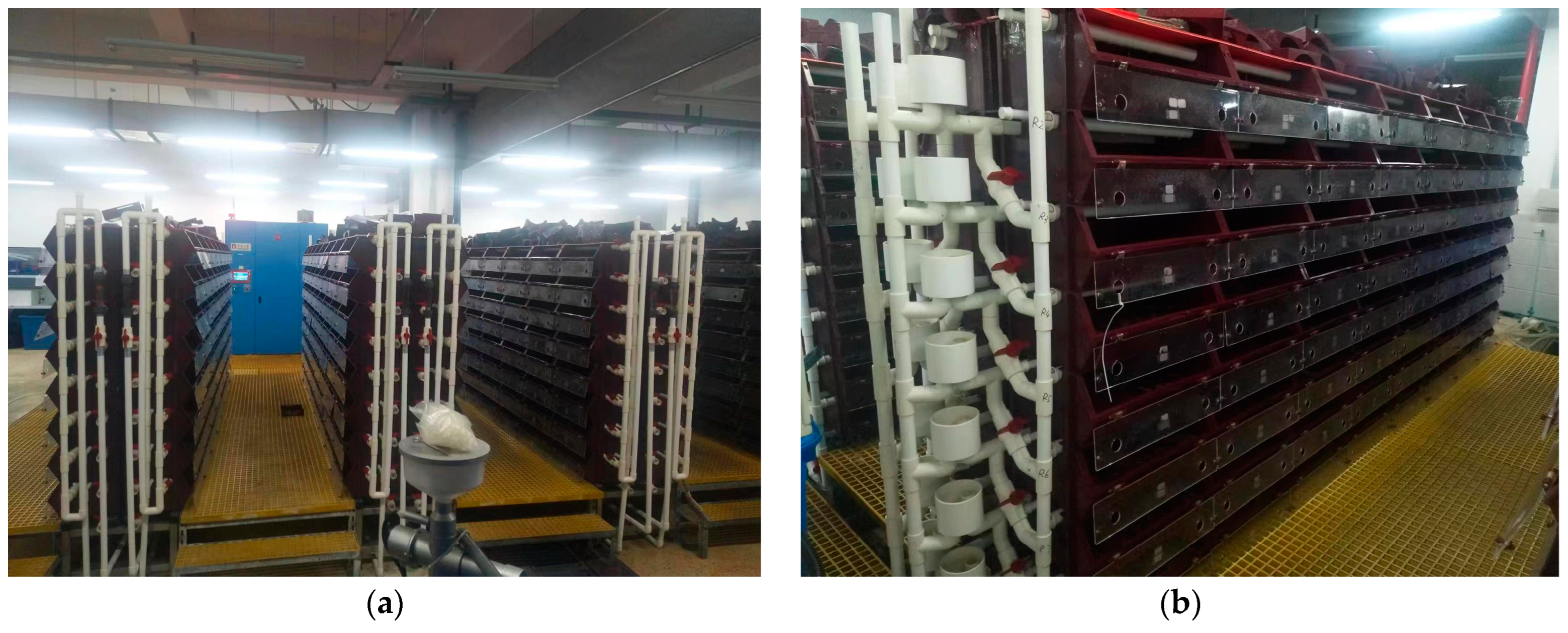
A new agricultural farming model known as single-frame three-dimensional aquaculture was created on the principle of circulating water and can be used to reuse aquaculture water, reduce agricultural energy use and environmental pollution, and realize the sustainable development of new agricultural technology. In light of the development of recirculating water culture technology [1], the Portunus three-dimensional apartment culture technology has become widely popular. According to Figure 1, each aquaculture frame corresponds to one Portunus; the frame is covered with sand, and the water depth of the frame is approximately 10–20 cm. Portunus are fed regularly and quantitatively using pellet feed or small fish and shrimp as bait for culture. Currently, a large number of daily inspections are handled manually in the factory-based single-frame three-dimensional culture. In order to improve the efficiency of farming, there is an urgent need for a new technological method to manage the daily inspections of large-scale three-dimensional aquaculture. On the other hand, machine vision, as an efficient method for automatic detection [2,3], has been widely used for behavioral detection, quantitative feeding, and feeding tracking in wisdom breeding [4,5,6]. For example, the fusion of images with mathematical models to increase the reliability of the acquired information, 3D coordinate models, and tracking infrared reflection (IREF) detection devices [7] for fish behavior detection. Based on machine learning, differences between one or more frames of the camera [8] are used to determine the differences in fish feeding and quantitative indicators of feeding. To increase the reliability of information acquisition and to reduce interference, the optical flow was used to extract behavioral features (speed and rotation angle) for feeding tracking [9]. Based on this, this paper addresses the inefficiency of manual inspections of large-scale single-frame three-dimensional culture by conducting a study on the survival rate judgment of Portunus based on visual detection. Identifying visual-feature parameters such as Portunus centroid movement, feed residual bait, and Portunus rotation angle in the frame were performed using machine vision technology. Further, the fusion of the three parameters was used to determine the survival rate of the Portunus.

The recognition of residual bait and Portunus centroid belongs to the target detection problem in visual inspection. In deep-learning target detection, a deeper network, richer feature annotation and extraction, and higher computing power are the key technical issues to improve target detection accuracy and real-time efficiency. Deeper networks can improve the accuracy of target detection, and Rauf [10] proposed to deepen the number of CNN convolutional layers with reference to the VGG-16 framework [11], which enabled the CNN to be extended from 16 to 32 layers and improved the accuracy of target recognition on the Fish-Pak dataset by 15.42% compared to the VGG-16 network. Richer feature annotation and network frameworks can improve learning efficiency. As the problem of aquaculture fish-action recognition arises, Måløy [12] proposed to use a CNN framework that combined spatial information and motion features fused with time-series information to provide richer information features related to fish behavior, with an accuracy of 80% in the task of predicting feeding and non-feeding behavior in fish farms. Combining network depth, higher feature extraction capability, and real-time requirements, the Faster R-CNN [13] and YOLO [14] frameworks have become the two leading algorithmic frameworks for target detection. They are widely used in crab target identification, fish target identification, and water quality prediction [15,16,17]. Faster R-CNN with an RPN network makes for high accuracy. Li [18] initialized the Faster R-CNN network using pretrained Zeiler and Fergus (ZF) models and optimized the convolutional feature map window for the ZF model network, resulting in improved detection speed and a 15.1% increase in mAP. YOLO is an end-to-end network framework that is fast and highly accurate. In order to identify fish species in deep water, Xu [19] performed experiments based on the YOLOV3 model [20] for fish detection in the high turbidity, high velocity, and murky water environment, and evaluated the fish detection accuracy in three datasets under marine and hydrokinetic (MHK) environments. It was shown that the mAP score reached 0.5392 under this dataset, and YOLOV3 improved the target detection accuracy. Due to the problem of unstable data transmission conditions in fish farms, Cai [21] used MobileNet to replace the Darknet-53 network in YOLOV3, which reduced the model size and the computation by a factor of 8–9. The speed of the optimized algorithm was improved, and the mAP was increased by 1.73% based on the fish dataset. Both Faster R-CNN and YOLO networks can extract deeper features from images, but YOLO belongs to the end-to-end algorithmic framework, which is faster. In large-scale three-dimensional factory farming, faster recognition algorithms mean real-time detection of targets in aquaculture. Therefore, the improved YOLO network was chosen for the recognition of residual bait and Portunus centroid targets.

The edge contour (rotation angle) recognition of Portunus belongs to the problem of visual inspection target segmentation. Aside from the traditional Canny and Pb algorithms, most target segmentation problems are now solved by architectures that use deep learning. Most of the time, different backbone network architectures and information fusion methods are made based on convolutional neural network frameworks like GooLeNet and VGG to pull out multi-scale features and achieve more accurate edge detection and segmentation. Typical backbone network architectures include multi-stream learning, skip-layer network learning, single model on multiple inputs, training independent network, holistically-nested networks, etc. In 2015, Xie [22] proposed the Holistically-Nested Edge Detection (HED) algorithm, which uses VGG-16 as the backbone network base, initializes the network weights using migration learning, and achieves simple contour segmentation of the target through multi-scale and multi-level feature learning. The HED algorithm achieves an ODS (optimal dataset scale) of 0.782 on the BSDS500 dataset, reflecting better performance of the dataset on the training set, achieving better segmentation results, and realizing target contour recognition. Subsequently, the Convolutional Oriented Boundaries (COB) algorithm [23] was improved on the basis of HED, which generates multi-scale, contour-oriented, regionally-high-level features for sparse boundary-level segmentation with an ODS of 0.79 on BSDS500, optimizing the training set contour information feature extraction. Further, to reduce the number of deep learning network parameters and maintain the spatial information in segmentation, Badrinarayanan [24] proposed SegNet, an encoder–decoder-based segmentation network architecture. The SegNet algorithm transfers the maximum pooling index to the decoder, improving the segmentation resolution. The SegNet algorithm moves the maximum pooling index to the decoder, improving the segmentation accuracy. The CEDN (Fully Convolutional Encoder–Decoder Network) algorithm [25] can detect higher-level object contours, further optimizing the encoder–decoder framework for contour detection, and the CEDN algorithm improves the average recall on the PASCAL VOC dataset from 0.62 to 0.67 and the ODS reached 0.79 on the BSDS500 dataset. In 2015, researchers found that the ResNet network framework [26] can extend the neural network depth and extract complex features efficiently. In 2019, Kelm [27] proposed the RCN network architecture based on the ResNet algorithm, which is used for contour detection by using multi-path refinement and fuses mid-level and low-level features in a specific order with a concise and efficient algorithm, thus becoming a leading framework for edge detection. For example, Abdennour [28] proposed a driver profile recognition system with 99.3% accuracy for facial profile recognition based on RCN networks.

In summary, the problem is the visual detection of the survival rate for Portunus’ three-dimensional apartment culture. The main work of this paper is as follows: (i) Based on YOLOV5, the residual bait and Portunus centroid were detected, and the EIOU loss [29] bounding box loss function was proposed on the basis of CIOU (Complete IOU) loss to optimize the accuracy of YOLOV5 in predicting the centroid moving distance of Portunus and residual bait. (ii) For the Portunus contour target segmentation problem, the RCN-based binary cross-entropy loss to double-threshold binary cross-entropy loss function is optimized to improve the Portunus contour detection accuracy and calculate the contour endpoint coordinates (i.e., rotation angle) to improve the Portunus contour curve accuracy. (iii) Based on YOLOV5’s RCN algorithm, Portunus centroid movement, residual bait, and rotation angle were three parameters identified, using locally weighted linear regression (LWLR) and the softmax algorithm for information fusion to give a comprehensive determination model of the Portunus survival rate.

The main innovation of this paper lies in the visual detection of three parameters that indirectly reflect the survival of the Portunus using machine vision technology, and the establishment of a single-parameter survival determination model and a three-parameter fusion determination model, respectively. Thus, a vision detection-based survival detection method for Portunus was given. Currently, most of the vision inspection techniques for Portunus are focused on target detection. In the context of three-dimensional culture, the visual-detection method of multi-parameter fusion has not been reported. Meanwhile, this paper uses the YOLOV5 algorithm to detect the centroid movement distance and residual bait of Portunus and the RCN algorithm to detect the rotation angle of Portunus. In residual bait recognition, pellet bait belongs to small target recognition; this paper uses the EIOU loss function to enhance the training mAP and improve the recognition accuracy of pellet bait and Portunus. In RCN for Portunus contour rotation angle recognition, this paper proposes a double-threshold loss function algorithm to reduce the loss function and improve the training accuracy. Finally, a combined three-parameter LWLR fusion determination algorithm was given, and the fused survival recognition accuracy was improved by 5.5%, relative to the single-parameter (average accuracy) recognition accuracy.

2. Materials and Methods

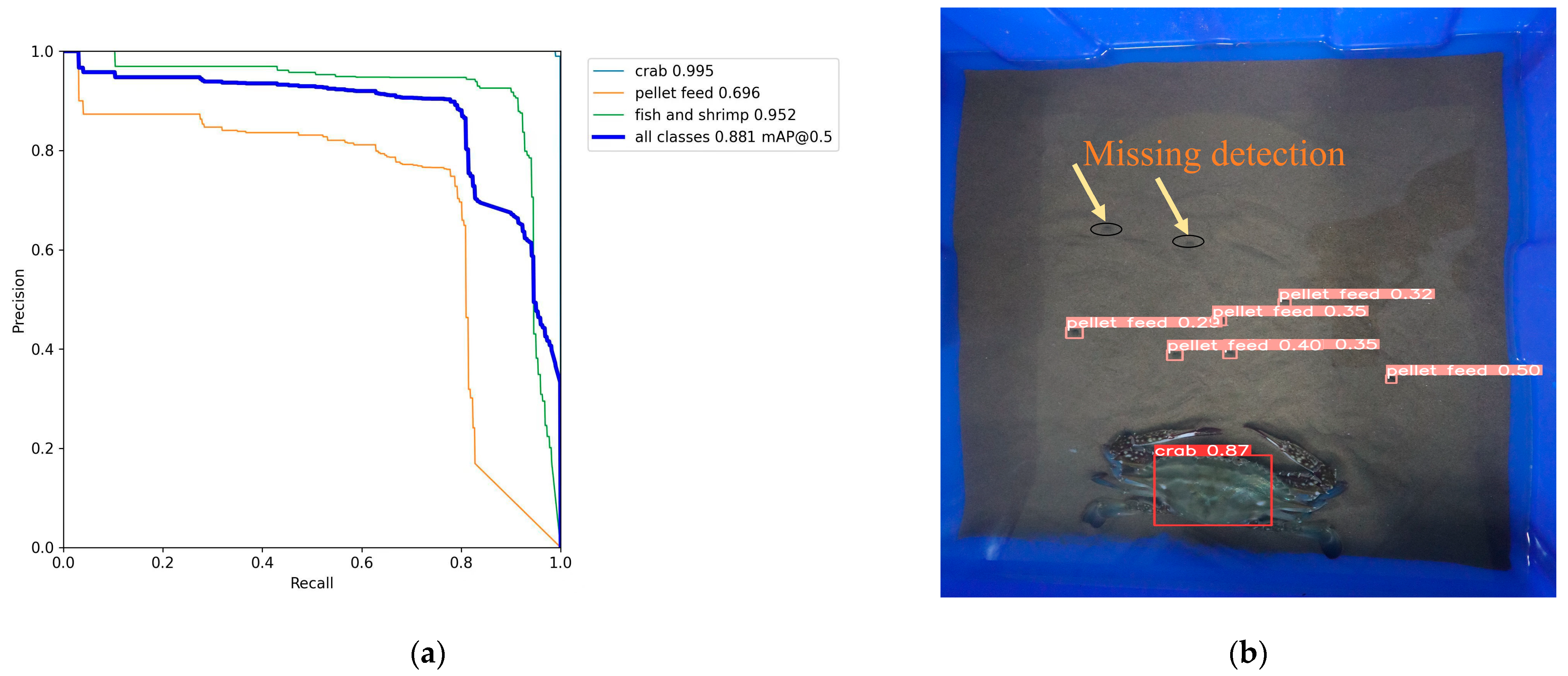
In this paper, YOLOV5 and the RCN framework are applied to visually detect movement of the Portunus centroid, bait, and rotation angle. In YOLOV5 small-pellet-feed vision detection, YOLOV5 has poor recognition ability for small targets because it usually uses the CIOU bounding box loss function. There will be missed detection during the visual inspection of pellet bait, fish, and shrimp feed, as shown in Figure 2. The YOLO5 detection algorithm with the CIOU bounding box loss function has a mAP (0.5) of 69.6% for pellet feed target identification and 95.2% for tiny fish and shrimp target recognition in experiments. The average target identification accuracy mAP (0.5) of Portunus, pellet feed, fish, and shrimp feed was 88.1%. As a result, the purpose of this research was to upgrade the CIOU bounding box loss function to the EIOU loss function in order to increase the detection accuracy of baited tiny objects such as pellet feed.

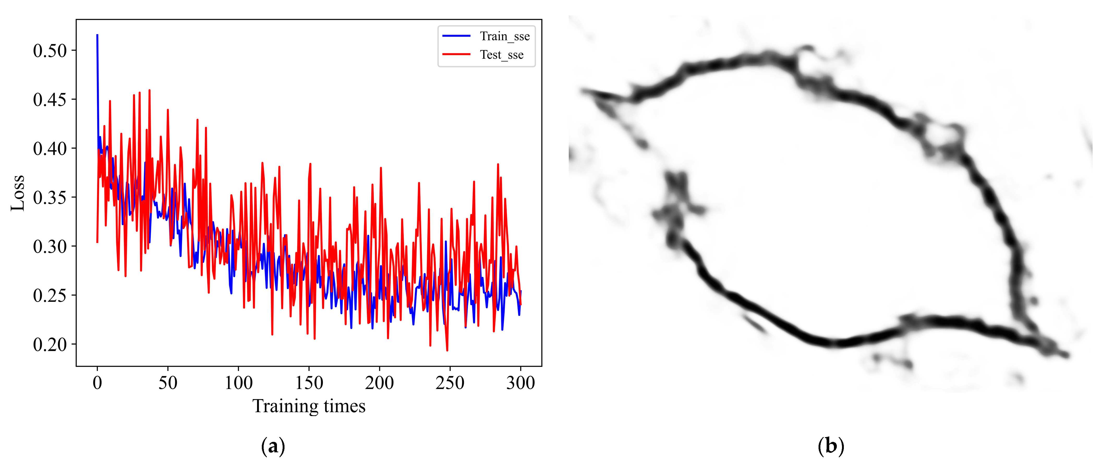
Furthermore, as shown in Figure 3, after training with 300 epochs in RCN Portunus rotation angle detection, the average loss of the training set and the average loss of the test set were determined to be 0.2857 and 0.3071, respectively. The test results had significant biases when compared to the training results, and the Portunus contour prediction was fuzzy with a contour missed-detection problem. In order to enhance Portunus target profile recognition, this work offers a double-threshold loss function based on the RCN algorithm.

2.1. Survival Rate Detection YOLOV5 and RCN Framework

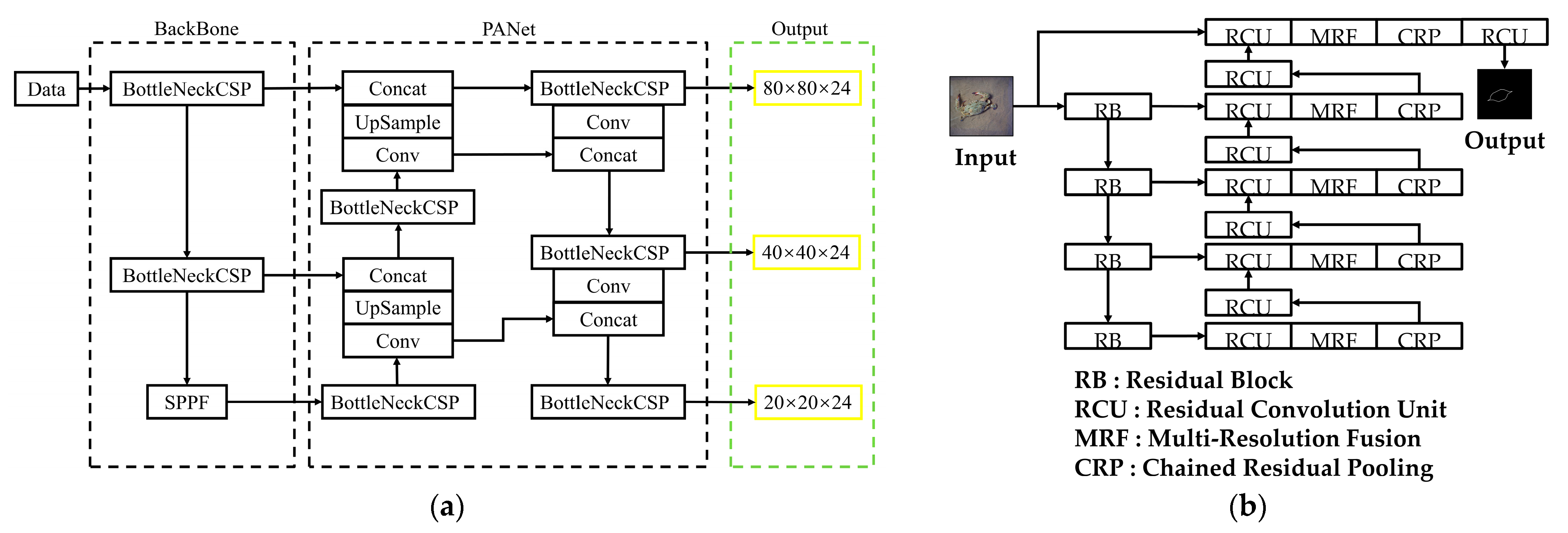
(1) Movement of the centroid and identification of residual bait based on YOLOV5. The movement of the Portunus’ centroid and the residual bait are indirect indicators of whether or not the Portunus is alive. The typical size of a Portunus farm breeding frame is 500 mm × 400 mm, and the size of the frame helps to identify residual bait and the centroid coordinates of the Portunus. YOLOV5 is an end-to-end algorithmic framework with criteria for both speed and accuracy of detection. As a result, this article is built on the YOLOV5 framework for target recognition of Portunus centroid movement and residual bait, and Figure 4a shows its network architecture.

As illustrated in Figure 4a, the YOLOV5 network structure consists of four major modules: Data, BackBone, PANet, and Output. Its loss is comprised of three components: the loss of Classes, Objectness, and Location, as well as identifying and detecting the Portunus and residual bait. The image data are labeled with 3 different targets using the labeling: Portunus, pellet feed, and fish and shrimp. After labeling, the .xml file is acquired, which is then translated to .txt file. With reference to the PASCAL VOC dataset, a Portunus target detection dataset was generated, of which 900 were used for training and 100 for validation. After preprocessing the photos to 640 × 640 size, 300 epochs of network training began. To boost training efficiency, the training Portunus dataset can be reclustered to build anchors templates based on the targets in the training Portunus dataset. In YOLOV5, data were preprocessed into the BackBone framework, and BackBone accelerated the extraction of Portunus and residual bait characteristics using convolutional networks. PANet performed same channel feature fusion and image size recovery after feature extraction. Lastly, three target detection layers were produced, reflecting the identification of small target objects, medium target objects, and big target objects, enhancing the accuracy of detecting Portunus and residual baits.

(2) Portunus rotation angle detection based on RCN. The angle of rotation of the Portunus is also an indirect indicator of whether or not the Portunus is alive. Due to the three-dimensional nature of single-frame Portunus culture, it is unlikely that Portunus will move in big ways. Instead, feeding is often accompanied by small movements and rotations in many directions. In this paper, the RCN framework is used to detect the Portunus contour, and the end-point coordinate approach is used to determine the Portunus rotation angle based on the end-point image coordinates that are detected. Figure 4b shows the architecture for RCN Portunus contour identification and rotation angle computation.

As illustrated in Figure 4b, the RCN network structure consisted of six major modules: Input, RB, RCU, MRF, and Output. Its loss function was binary cross-entropy loss, which was also a crucial aspect in the identification of Portunus contours. The image data were labeled with crab by LabelMe, and after labeling, .json files were obtained, which were further transformed into outline.jpg files. The Portunus contour dataset was created with reference to the BSDS500 dataset, and 416 photos from the dataset were used for training, 93 for testing, and 11 for validation. After preprocessing the images to 640 × 640 size, 300 epochs of network training began to train the Portunus contour dataset with continuous learning to increase contour prediction efficiency. To improve contour feature extraction, data were preprocessed into the RB framework in the RCN algorithm. As the Portunus contour features were retrieved, they entered the RCU framework with a residual convolution layer, which can enrich the network parameters while also adjusting and correcting the MRF input. After that, the convolutional MRF framework and upsamples were placed on the feature map channels and sizes in order to combine Portunus contour feature maps of various resolutions. Next, the CRP framework used chained convolution and pooling, which can better aggregate more information about the Portunus contours. Finally, on the basis of six CNN modules, a profile image of the Portunus crab was produced.

(3) Computation of rotation angle using the end-point coordinate approach. When the RCN detected the Portunus shape, the end-point coordinate method was used to determine the Portunus selection angle, as illustrated in Figure 5. First, Figure 5a shows the minimal outside rectangular box of the Portunus contour, and Figure 5b shows the coordinates of the Portunus tip point based on the outer rectangular box. After that, the coordinates of the contour tip points A and B as well as the Portunus’ rotation angle were determined, as illustrated in Figure 5c.

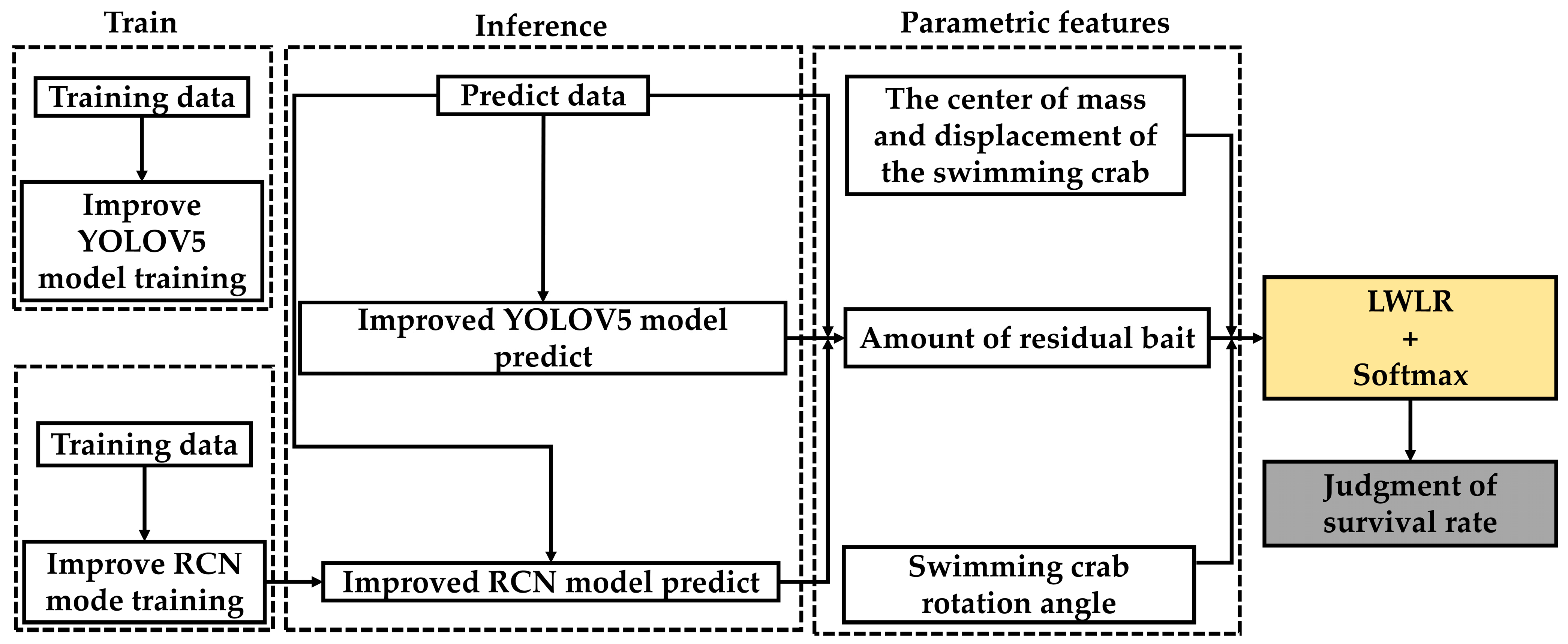
(4) For Portunus survival, the single-parameter determination model and multi-parameter fusion determination model were proposed. This paper used the YOLOV5 and RCN algorithms to identify the three parameters of Portunus centroid movement distance, residual bait ratio, and rotation angle. Next, the survival rate determination model of Portunus survival (single parameter) was created using the LWLR method. Finally, the softmax method was used to produce the regression prediction model of Portunus survival rate. Figure 6 shows the general structure of the Portunus survival fusion judgment model.

LWLR is a non-parametric machine learning algorithm, and the regression coefficients $\hat{w}$ are fitted to each sample of centroid movement distance, residual bait, and rotation angle. The visual recognition parameters of Portunus centroid movement distance, residual bait ratio, and rotation angle are $c_1$, $c_2$, and $c_3$, respectively. Take the $c_1$ parameter as an example, and randomly select its value as 350. Inputting the values of $c_1$ from the target detection into expression (1) provides the $x_{1c}$ feature matrix expression as:

$$x_{1c}=\left[c_1{}_1,c_{12},\cdots c_{1n}\right]$$

(1)

where n is generally denoted as the number of sample features, and $c_1{}_n$ is denoted as different features. The characteristic matrix expression of the training sample set is as follows:

$$X_c={\left[c_1{}^{\left(1\right)}\cdots c_1{}^{\left(m\right)}\right]}^{{\rm T}}$$

(2)

where m = 350 represents the sample size of the training set, and $c_1{}^{\left(m\right)}$ represents the sample size. The labels of training samples are as follows:

$$Y_c={\left[y_c{}^{\left(1\right)}\cdots y_c{}^{\left(m\right)}\right]}^{{\rm T}}$$

(3)

where $y_c{}^{\left(m\right)}$ represents the true label of each sample size. Then, the prediction formula of LWLR for a single feature sample is as follows:

$$H_{\widehat{w}}\left(c\right)=x_{1c}\widehat{w}={\displaystyle \sum _{k=1}^n{x}_{1k}{\widehat{w}}_k}$$

(4)

where $\hat{w}$ represents the regression coefficient, the expression is as follows:

$$\widehat{w}={\left(X_c{}^{T}W{X}_c\right)}^{-1}{X}_c{}^{T}W{Y}_c$$

(5)

where W is the diagonal matrix of m×m, and each data point is given a weight. LWLR uses “kernel” to give higher weight to nearby points. In this paper, Gaussian kernel is selected to construct the weight matrix W, and the expression is as follows:

$$W\left(i,i\right)=\mathit{exp}\left[\frac{{\left|c_1{}^i-c_1\right|}^2}{-2k^2}\right]$$

(6)

where $W\left(i,i\right)$ represents the diagonal element of W, and $i$ in $c^i$ represent the weight value of the training sample, and its range is $\left(0,1\right]$. Among them, $c_1$ represents the reference point and $c_1^i$ represents the predicted value sample. Parameter k determines how much weight is given to nearby points. When k is determined, the one-parameter survival rate determination model for $c_1$ is achieved.

2.2. YOLOV5 Boundary Box Loss Function EIOU

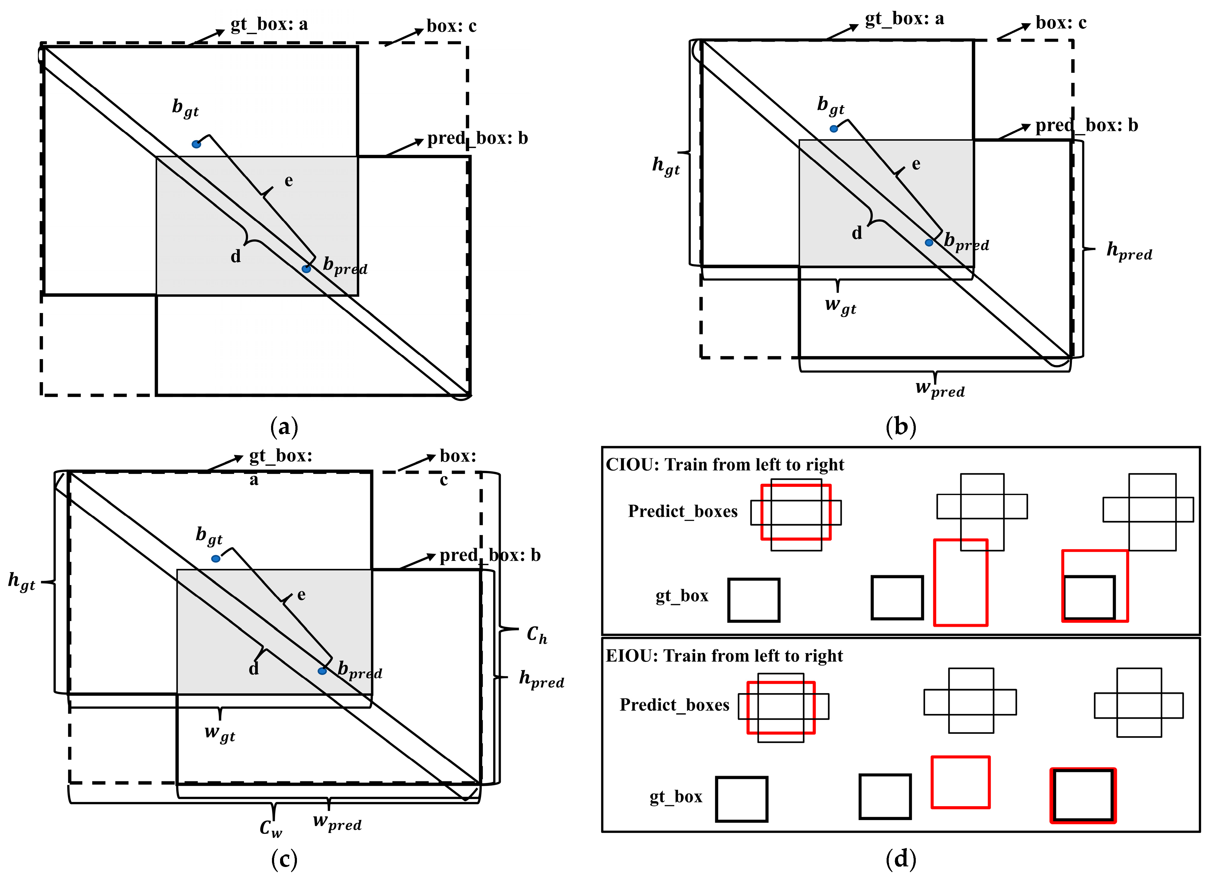
Due to YOLO bounding box loss, it experienced SSE Loss, IOU Loss [30], GIOU Loss [31], DIOU Loss [32], and CIOU Loss. The two factors of bounding box to be solved with DIOU were overlapping area and center point distance. DIOU is shown in Figure 7a, and the expression of DIOU is as follows:

$$DIOU=IOU-\frac{{\rho }^2\left(b_{pred},b_{gt}\right)}{d^2},Los{s}_{DIOU}=1-DIOU$$

(7)

where $b_{\mathit{pred}}$ and $b_{gt}$ represent the center point coordinates of the predicted box and the center point coordinates of the real box, respectively; $\rho$ represents the Euclidean distance, namely $e^2={\rho }^2(b_{\mathit{pred}},b_{gt})$; and d represents the diagonal distance of the smallest circumscribed rectangular box. DIOU not only solves the large error problem between the GIOU prediction box and real box, but also makes the relative distance between the prediction box and real box clear. However, there is no aspect ratio factor in DIOU function, and the aspect ratio influence factor $\alpha v$ (i.e., CIOU) is added on the basis of DIOU, as shown in Figure 7b. The expression for CIOU is as follows:

$$CIOU=IOU-\frac{{\rho }^2\left(b_{pred},b_{gt}\right)}{d^2}-\alpha v=DIOU-\alpha v,Los{s}_{CIOU}=1-CIOU$$

(8)

where the expression for v is as follows:

$$v=\frac{4}{{\pi }^2}{\left(\mathit{arctan}\frac{w_{gt}}{h_{gt}}-\mathit{arctan}\frac{w_{pred}}{h_{pred}}\right)}^2$$

(9)

where $v$ is used to measure the consistency of aspect ratio, and $\alpha$ is the value of equilibrium $v$ which can be expressed as:

$$\alpha =\frac{v}{1-IOU+v}$$

(10)

The formula for measuring the aspect ratio in CIOU is relatively complex, and the aspect ratio cannot replace the width and height of bounding box ($w=k{w}_{gt}$, $h=k{h}_{gt}$ leads to $v$ being 0). The partial derivatives of w and h in v are obtained, respectively, of which relationship is as follows:

$$\frac{\partial v}{\partial w}=-\frac{h}{w}\ast \frac{\partial v}{\partial h}$$

(11)

Therefore, width and height can only take the opposite number in the optimization process. The difference of aspect ratio reflected by Formula (11) v is not the real difference between width, height, and confidence, so the training and prediction accuracy of tiny objects decreases or even misses. The EIOU bounding box loss function, on the basis of CIOU, is proposed to replace the width and height losses, as shown in Figure 7c. $\alpha v$, as shown in Figure 7c. The improved EIOU formula is as follows:

$$EIOU=IOU-\frac{{\rho }^2\left(b_{pred},b_{gt}\right)}{d^2}-\frac{{\rho }^2\left(w_{pred},w_{gt}\right)}{c_w^2}-\frac{{\rho }^2\left(h_{pred},h_{gt}\right)}{c_h^2},Los{s}_{EIOU}=1-EIOU$$

(12)

where $w_{\mathit{pred}}$ and $w_{gt}$ represent the width of the predicted label and the width of the real label, $h_{\mathit{pred}}$ and $h_{gt}$ represent the height of the predicted label and the height of the real label, and $c_w$ and $c_h$ represent the width and height of the minimum external rectangular frame. Obviously, EIOU loss directly minimizes the width and height difference between the predicted bounding box and the real bounding box, and has better positioning and recognition effect for small objects. Moreover, $Los{s}_{EIUO}$ accelerates the convergence and improves the regression accuracy, and increases the mAP for small object detection. The comparison between CIOU and EIOU recognition is shown in Figure 7d.

2.3. RCN Double-Threshold Loss Function

The fundamental cause of fuzzy RCN Portunus contour prediction and missed contour detection is a lack of feature information extraction in the RCN loss function, and the binary cross-entropy loss function:

$$L\left(h_{\theta }\left(x\right),y\right)=-y\cdot weights\cdot \mathit{log}\left(h_{\theta }\left(x\right)\right)-\left(1-y\right)\mathit{log}\left(1-h_{\theta }\left(x\right)\right)$$

(13)

where $h_{\theta }\left(x\right)\in \left[0,1\right]$, $y\in \left\{0,1\right\}$, $weights=10$, and $h_{\theta }\left(x\right)$ obtained the corresponding binary label through the prediction of pixel x. When the value of weights is fixed, inadequate feature extraction due to multiple convolutional stacking and upsampling fusion may lead to the inaccurate capturing of contour information, blurred contours, or missed contour detection of the Portunus. In this paper, the value of weights in the RCN loss function were optimized through the double-threshold RCN loss function. The double-threshold binary cross-entropy loss function is defined as follows:

$$\{\begin{array}{cc}weights0=A& h_{\theta }\left(x\right)\ge a\\ weights0=B& h_{\theta }\left(x\right)<a\end{array},\{\begin{array}{cc}weights1=A& h_{\theta }\left(x\right)\ge b\\ weights1=B& h_{\theta }\left(x\right)<b\end{array}$$

(14)

$$\{\begin{array}{l}{L}_0\left(h_{\theta }\left(x\right),y\right)=-y\cdot weights0\cdot \log \left(h_{\theta }\left(x\right)\right)-\left(1-y\right)\mathit{log}\left(1-h_{\theta }\left(x\right)\right)\\ L_1\left(h_{\theta }\left(x\right),y\right)=-y\cdot weights1\cdot \log \left(h_{\theta }\left(x\right)\right)-\left(1-y\right)\mathit{log}\left(1-h_{\theta }\left(x\right)\right)\end{array}$$

(15)

$$L\left(h_{\theta }\left(x\right),y\right)=c\cdot L_0\left(h_{\theta }\left(x\right),y\right)+d\cdot L_1\left(h_{\theta }\left(x\right),y\right)$$

(16)

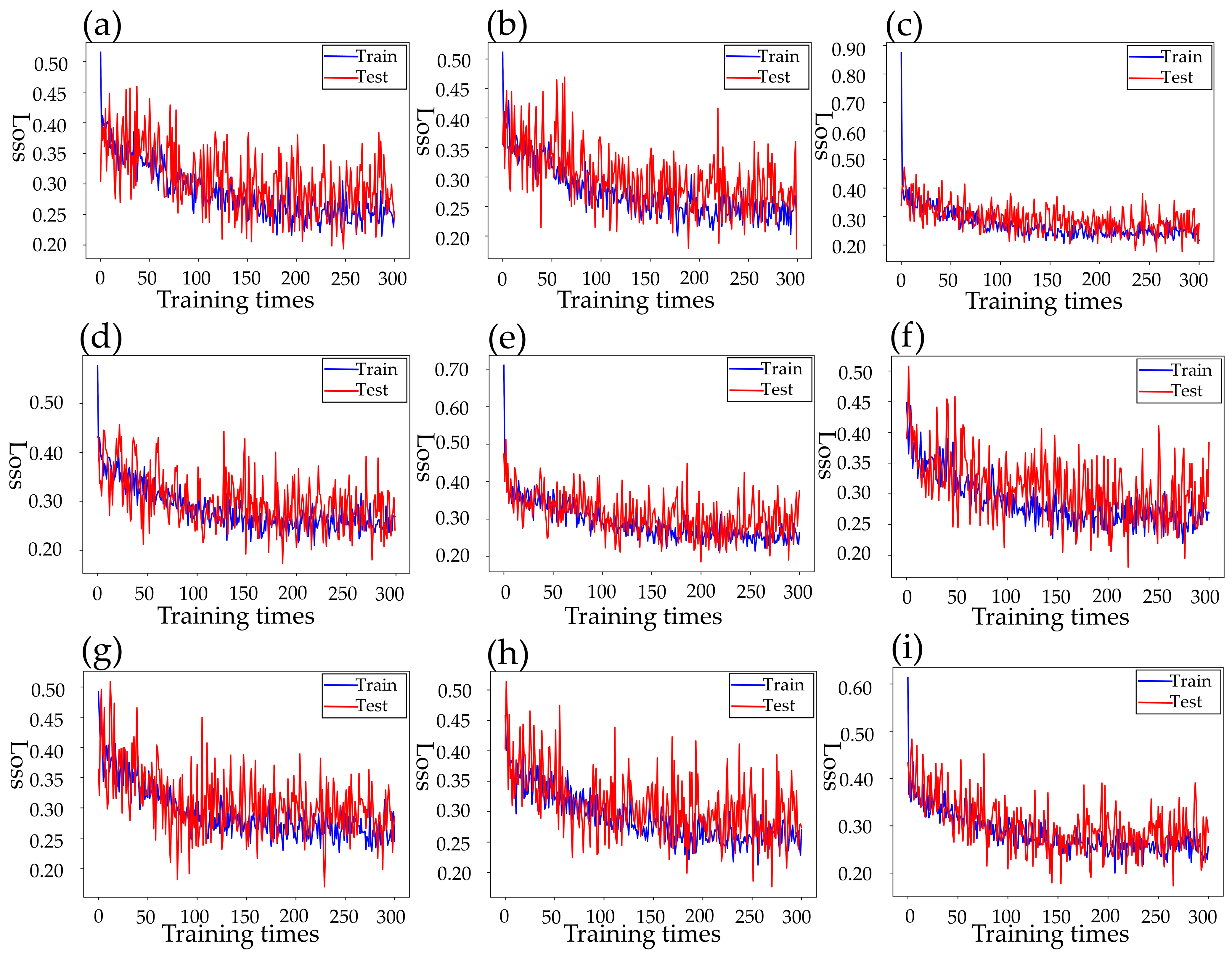
where a, b, c, and d are hyperparameters, and the values of A and B are 10 and 1, respectively. The double-threshold binary cross-entropy loss function, which can improve edge learning and extraction in convolutional neural networks, can effectively prevent the loss of key contour edge information. Moreover, the value of weights can be realized by setting the thresholds $h_{\theta }\left(x\right)$. To acquire a clear contour of Portunus, $\left\{a,b\right\}$ hyperparameters take the values of $\left\{0.99,0.95\right\}$, $\left\{0.98,0.94\right\}$ and $\left\{0.97,0.93\right\}$, respectively, for comparative experiments. $\left\{c,d\right\}$ hyperparameters take the values of $\left\{0.6,0.4\right\}$, $\left\{0.7,0.3\right\}$, and $\left\{0.8,0.2\right\}$ for cross-comparison experiments. Referring to the number of pictures in the BSDS500 contour dataset, 416 training sets, 93 test sets, and 11 validation sets were established, with 300 RCN training times.

Figure 8a–c show the training and test loss function curves when the hyperparameter $\left\{a,b\right\}$ takes the value of $\left\{0.99,0.95\right\}$ and the hyperparameters $\left\{c,d\right\}$ take the values of $\left\{0.6,0.4\right\}$, $\left\{0.7,0.3\right\}$, and $\left\{0.8,0.2\right\}$, respectively. Learning from Figure 8a–c, when the hyperparameters $\left\{c,d\right\}$ take the values of $\left\{0.6,0.4\right\}$, $\left\{0.7,0.3\right\}$, and $\left\{0.8,0.2\right\}$, the average loss of the training set and test set are 0.2735 and 0.2932, 0.2736 and 0.2967, and 0.2743 and 0.2879, respectively, with the optimal value of $\left\{0.8,0.2\right\}$ from this group being $\left\{c,d\right\}$.

Figure 8d–f show the training and test loss function curves when the hyperparameter $\left\{a,b\right\}$ takes the value of {0.98,0.94} and the hyperparameters $\left\{c,d\right\}$ take the values of $\left\{0.6,0.4\right\}$, $\left\{0.7,0.3\right\}$, and $\left\{0.8,0.2\right\}$, respectively. Learning from Figure 8d–f, when the hyperparameters $\left\{c,d\right\}$ take the values of $\left\{0.6,0.4\right\}$, $\left\{0.7,0.3\right\}$, and $\left\{0.8,0.2\right\}$, the average loss of training set and test set are 0.2855 and 0.3013, 0.2896 and 0.3114, and 0.2876 and 0.3095, respectively, with the optimal value of $\left\{0.6,0.4\right\}$ for this group being $\left\{c,d\right\}$.

Figure 8g–i show the training and test loss function curves when the hyperparameter $\left\{a,b\right\}$ takes the value of $\left\{0.97,0.93\right\}$, and the hyperparameters $\left\{c,d\right\}$ take the values of $\left\{0.6,0.4\right\}$, $\left\{0.7,0.3\right\}$, and $\left\{0.8,0.2\right\}$, respectively. Learning from Figure 8g–i, when the hyperparameters $\left\{c,d\right\}$ take the values of $\left\{0.6,0.4\right\}$, $\left\{0.7,0.3\right\}$, and $\left\{0.8,0.2\right\}$, the average loss of the training set and test set are 0.2915 and 0.3093, 0.2890 and 0.3106, and 0.2833 and 0.2999, respectively, with the optimal value of $\left\{0.8,0.2\right\}$ for this group being $\left\{c,d\right\}$.

The results of cross experiment are shown in

Table 1. Parameter selection comparison.

Parameter	Data
a, b, c, d	{a,b} = {0.99,0.95}	{a,b} = {0.98,0.94}	{a,b} = {0.97,0.93}
	{c,d} = {0.8,0.2}	{c,d} = {0.6,0.4}	{c,d} = {0.8,0.2}
Average loss	Train = 0.2743	Train = 0.2855	Train = 0.2833
	Test = 0.2879	Test = 0.3013	Test = 0.2999

with the optimal values of $\left\{a,b\right\}$:$\left\{0.99,0.95\right\}$,$\left\{c,d\right\}$:$\left\{0.8,0.2\right\}$.

2.4. LWLR Single-Parameter Survival Determination Model Computation

Actual measurement data were collected at the farm base for the Portunus contour dataset used in this study. A total of 500 data points were collected for each characteristic parameter of Portunus residual bait ratio, centroid moving distance, and rotation angle. Combined with the experience of aquaculture personnel: (i) The smaller the residual bait ratio, the greater the survival probability of Portunus under a certain feeding amount at each stage. The residual bait ratio is negatively connected to survival. (ii) Since the size of breeding frame is known (the maximum diagonal distance is 60 cm), the larger the centroid moving distance is, the greater the survival probability of Portunus. The threshold value of centroid moving distance is fixed as 13 cm (greater than the threshold survival of 100%). The centroid moving distance is positively connected to survival. (iii) The larger the rotation angle of Portunus, the higher the survival rate. The rotation angle is positively connected to survival. The paper chose the rotation angle threshold of 100° (greater than the threshold survival rate of 100%). The above three datasets are mutually independent from each other, as shown in

Table 2. Centroid movement distance, residual bait, and rotation angle datasets are partially displayed.

Characteristic	Data
A1	24.1713	19.2784	3.2957	4.1385	23.5104	13.5613	7.5881	…
Survival rate	0.9998	0.9987	0.4656	0.5115	0.9987	0.9912	0.6855	…
A2	0.7215	0.4191	0.9722	0.7203	0.9475	0.3074	0.0313	…
Survival rate	0.606	0.834	0.107	0.557	0.1490	0.8840	0.9624	…
A3	30.4562	80.5426	15.9573	25.3836	6.0410	35.661	80.5888	…
Survival rate	0.4035	0.90646	0.22009	0.3505	0.08081	0.45951	0.90617	…

A₁: The distance the Portunus’ centroid movement; A₂: Residual bait; A₃: The spin angle of the Portunus.

.

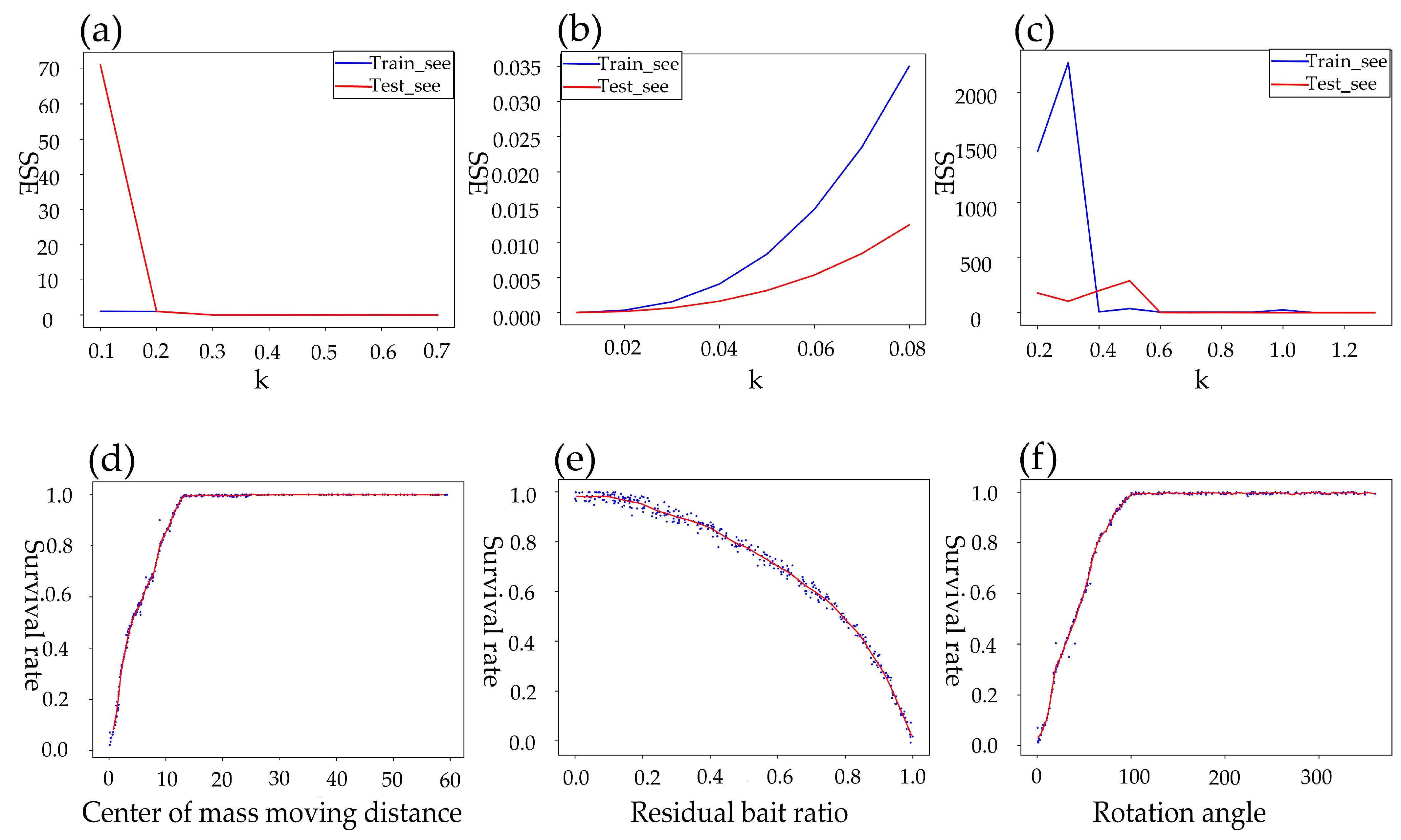
There are generalized linear connections between visual-detection feature parameters and Portunus survival rate. The value of k in $\widehat{w}$ must be calculated in advance in the single-parameter LWLR determination model training, since this decides whether the LWLR model is suitable and is the only hyperparameter that must be established in LWLR. SSE (Sum of Squared Errors) was applied to train both training and test sets, and parameter regression was conducted. The formula of SSE loss function is as follows:

$$SSE={\displaystyle \sum _{i=1}^m{\left(y_i-\widehat{y}\right)}^2}$$

(17)

where $\widehat{y}$ and $y_i$ are predicted value and true value of three characteristic parameters, respectively. The training set and test set are divided by 7:3 to obtain the residual bait ratio, centroid moving distance, and rotation angle. The text selects the appropriate value of k through the training and test set loss curves, which is as shown in Figure 9a–c. Learning from Figure 9a–c, the best values of k of the centroid moving distance, residual bait ratio, and rotation angle of Portunus through the LWLR model are 0.3, 0.02, and 1.1, respectively. Figure 9d–f shows the final one-parameter—the LWLR survival determination model.

3. Results

3.1. YOLO5–EIOU Boundary Frame Loss Experiment

In the YOLO5 frame for Portunus residual bait and centroid movement, the application of EIOU bounding box may significantly enhance the identification accuracy of tiny pellet bait, fish, and shrimp bait, and the survival rate determination accuracy of Portunus. In this paper, the YOLO5 algorithm using EIOU was experimentally verified.

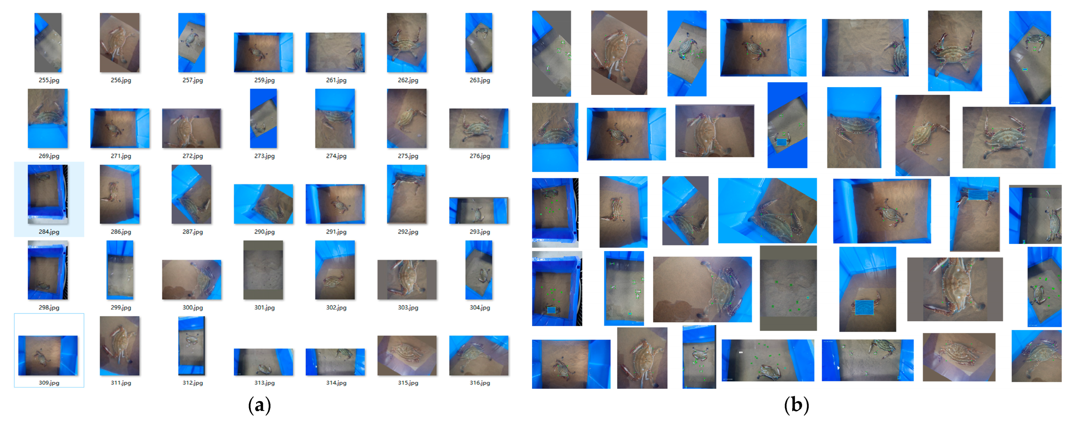
Firstly, the data of object detection were mainly from the photos before and after feeding. One thousand photos were marked with three different goals: Portunus, pellet feed, and small fish and shrimp feed using labeling software, with 90% training and 10% verification. The image set is shown in Figure 10.

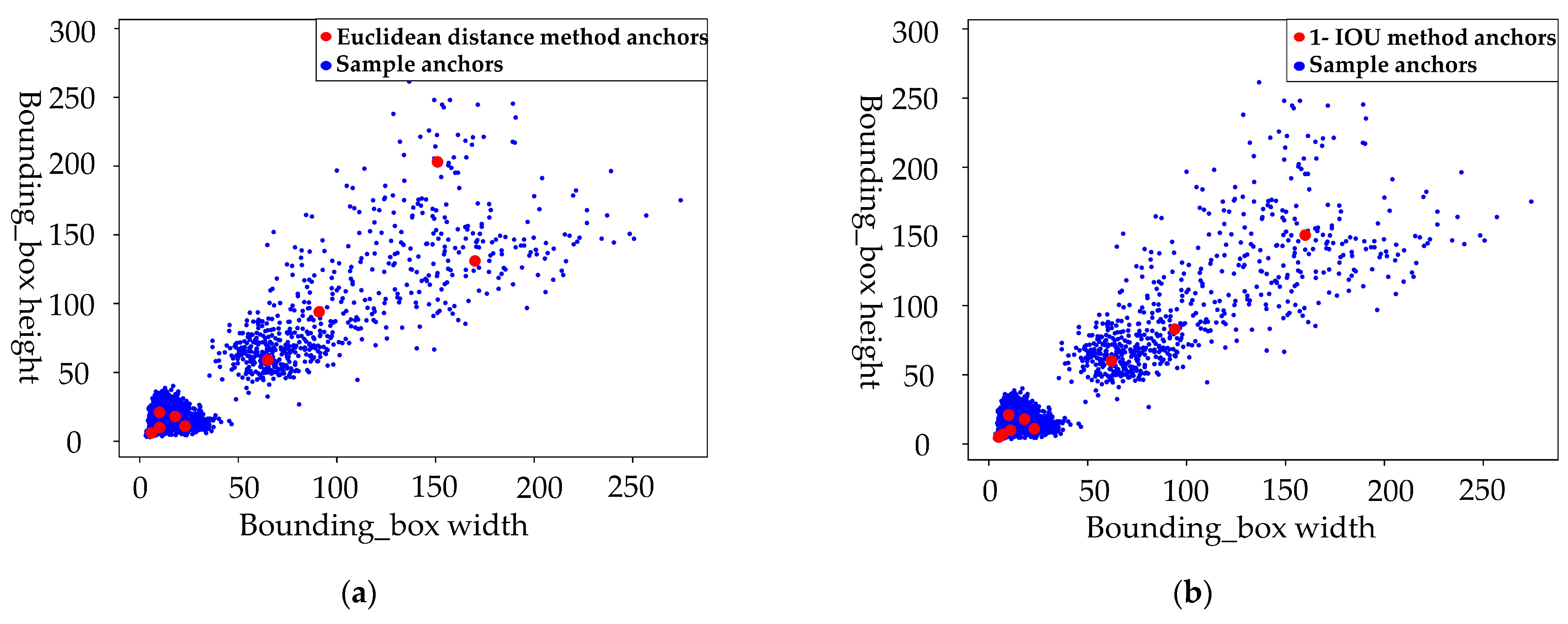
The selection of suitable data clustering center anchors in the YOLOV5 detection algorithm can significantly increase detection accuracy. As a result, prior to training, the k-means approach was used to examine the clustering of the Portunus dataset’s bounding box coordinate information in order to determine the best clustering centers of the dataset. The algorithm flow is as follows: (i) k samples were randomly selected from all samples as the initial center of the cluster, and they were not repeated. (ii) The distance of each sample from the center of each cluster was calculated, and different samples were assigned to the nearest cluster. (iii) The mean value of all samples in each cluster was calculated as a new cluster center. (iv) Steps ii and iii were repeated until there was no change or little change in the cluster center.

Meanwhile, in the k-means clustering analysis, the distance between bounding boxes and cluster center anchors was calculated using 1-IOU (bboxes, anchors) in this study. When the border frame and the matching cluster center IOU are larger, the distance between them is smaller. The clusters identified by comparing the 1-IOU with the Euclidean distance computation were as follows: [5, 5, 7, 7, 11, 10], [10, 21, 23, 11, 18, 18], [62, 60, 94, 83, 160, 151] and [6, 6, 10, 10, 10, 21], [23, 11, 18, 65, 59], [91, 94, 170, 131, 151, 203] with 1-IOU (bboxes, anchors) and Euclidean distance calculation clustering. The clustering results are shown in Figure 11a,b. The 1-IOU and Euclidean distance clustering indices have fitness values of 0.810 and 0.791, respectively. 1-IOU clustering anchors are more consistent with a realistic dataset sample distribution.

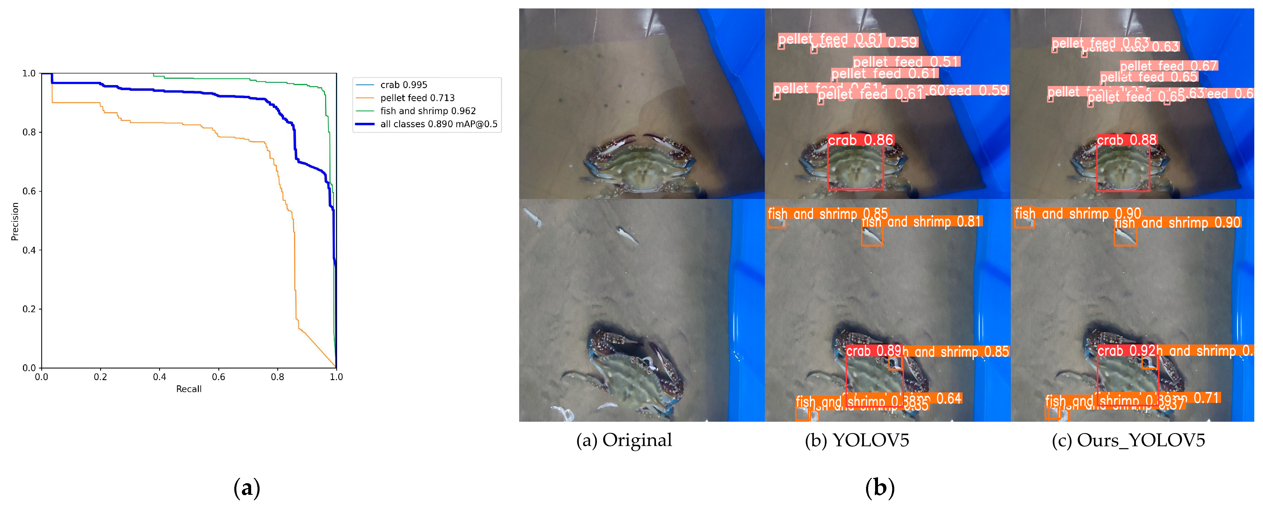
After the clustering analysis, the training and testing configuration data of YOLOV5 residual bait and Portunus centroid mass center recognition are shown in

Table 3. Experimental environment configuration.

Categories	Type
CPU	Intel(R) Core(TM) i9-10920X
RAM	64GB
Graphics card	NVIDIA GeForce RTX 3070
System	Windows 10
GPU Accelerate	cuda 11.3.1 cudnn8.2.1

. Comparing the network performance of YOLOV5 under CIOU loss and EIOU loss loss functions, the mAP (0.5) values for pellet feed, fish and shrimp after optimal identification using EIOU loss were 71.3% and 96.2%, respectively, as shown in Figure 12a. Compared to the CIOU loss loss function, the mAP(0.5) values for pellet feed, fish, and shrimp increased by 1.7% and 1%, respectively.

Table 4. Algorithm performance ratio table.

Index	Precision	Recall	mAP (0.5)	mAP (0.5:0.95)
YOLOV5	0.872	0.902	0.881	0.422
Ours_YOLO	0.892	0.883	0.890	0.440

shows a comparison of the algorithm performance training outcomes. The precision and IOU (threshold 0.5:0.95:0.05) mAP of target detection increased by 2% and 1.8%, respectively. EIOU loss improvement improved the average recognition accuracy of the whole picture, as demonstrated in Figure 12b.

3.2. RCN Double-Threshold Binary Cross-Entropy Loss Contour Recognition Experiment

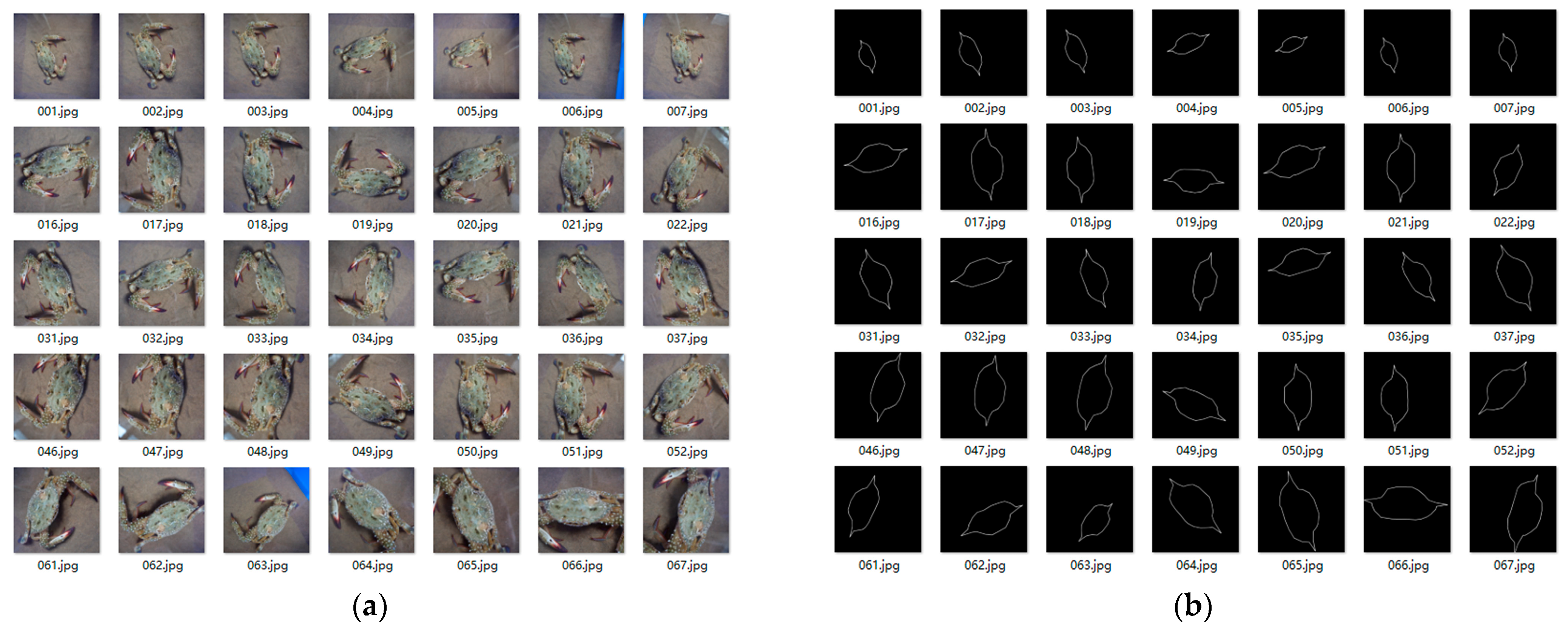
To address the issue of inaccurate Portunus contour recognition information, fuzzy contour, or missing contour detection in RCN Portunus contour recognition in this paper, we proposed a double-threshold binary cross-entropy loss. The experimental picture collection was the same as for YOLOV5 residual bait identification, and the contour dataset was labeled using LabelMe to differentiate between foreground and background and generate.json contour label files. The top section of the crab shell was serrated during the marking process, which may easily generate negative consequences such as reverse noise transmission during training. As a result, during the dataset labeling process, the crab shell (with serrated form) was flattened and tagged. In reference to the number of images in the BSDS500 contour dataset, this research labels 520 Portunus contour datasets. The training set, test set, and validation set accounted for 80%, 17%, and 3%, respectively. The image set is shown in Figure 13.

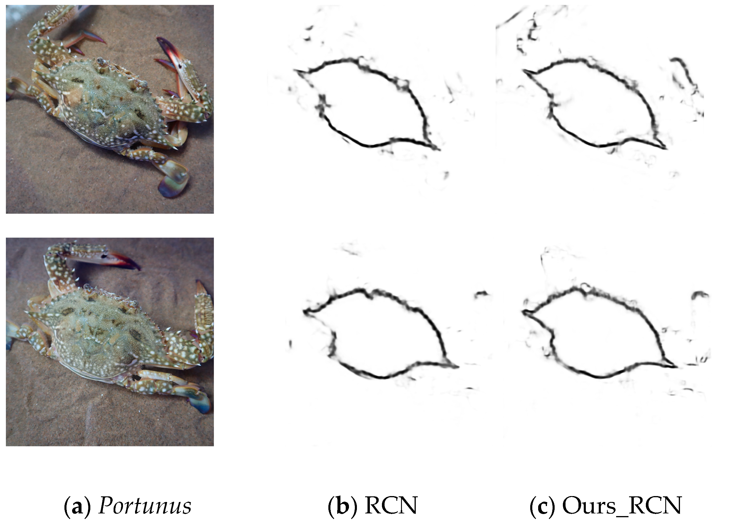
The binary cross-entropy loss function-based RCN network was trained using 300 epochs and the labeled image set; the average loss of the training set was 0.2857 and the average loss of the test set was 0.3071. Moreover, based on the improved double-threshold binary cross-entropy loss function RCN network after 300 training epochs, the average loss of the training set was calculated to be 0.2743, the average loss of the test set was 0.2879, and the optimized loss was reduced by 4% compared to that before optimization. On the other hand, the preoptimization RCN network required roughly 500 epochs to reduce the loss to 0.23. The optimized RCN can reduce the loss to 0.20 after training with 300 epochs. After algorithm improvements, the RCN network minimized contour blurring and missed contour detection phenomena while improving RCN prediction accuracy.

Table 5. Algorithm performance comparison.

Index	ODS	OIS	AP
CEDN	0.627	0.643	0.652
RCN	0.704	0.755	0.623
Our-RCN	0.724	0.768	0.631

compares and analyzes the ODS metrics, OIS metrics, and AP of the CEND network, the preoptimized RCN network, and the optimized RCN network in order to demonstrate the benefits of the algorithm enhancement. The optimized RCN algorithm improved the ODS and IOS by 2% and 1.3%, respectively. Finally, comparing the RCN loss function before and after optimizing, the contour prediction of Portunus is shown in Figure 14.

3.3. Multi-Parameter Survival Judgment Model

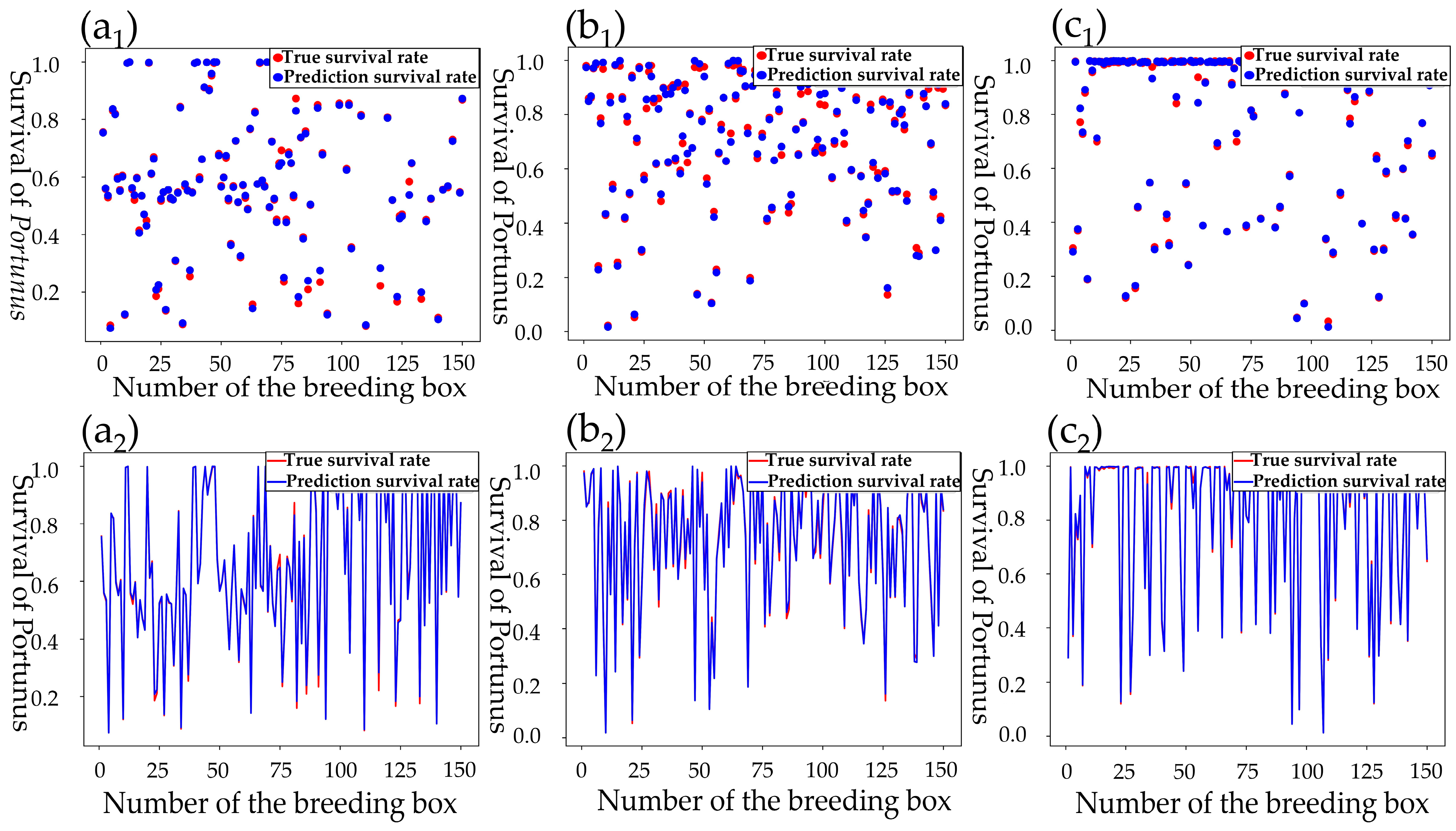
Following image-based identification of the Portunus’ centroid, rotation angle, and residual bait using the YOLOV5 and RCN algorithms, the bait’s residual concentration was calculated. In this paper, a single-parameter survival determination model was developed using LWLR. Experiments on the survival rate of Portunus under the effect of single characteristics were investigated. The 500 datasets were divided into training and test sets using 7:3. Figure 15a–c show the predicted and real values of the three image identification feature parameters of centroid moving distance, residual bait ratio, and rotation angle, respectively. As shown in Figure 15, the accuracy of each single parameter prediction was more than 80%, which is as shown in

Table 6. Accuracy rate under single parameter.

Parameter	Centroid Distance	Residual Bait Ratio	Rotation Angle
Accuracy	0.920	0.840	0.955

. To further improve the prediction accuracy, the $soft\mathit{max}\ast c$ algorithm was used to fuse the three feature parameters for prediction. The $soft\mathit{max}\ast c$ algorithm regression prediction formula for Portunus survival rate is as follows:

$$Logisti{c}_{prediction}={\displaystyle \sum _{k=1}^{k=3}soft\mathit{max}}\left(z_k\right)\ast c_k={\displaystyle \sum _{k=1}^{k=3}\frac{e^{z_k}}{e^{z_1}+e^{z_2}+e^{z_3}}}\ast c_k,z_k=\frac{c_k}{\partial -c_k},k=1,2,3$$

(18)

where $c_k$ is the single-parameter LWLR model survival rate; $\partial \in \left[1,2\right)$ hyperparameter is the scaling factor of $z_k$, and is the threshold for multi-parameter fusion. Gridding was used to pick several values of $\partial$, and the fusion of centroid moving distance, residual bait ratio, and Portunus rotation angle feature parameters were used to generate the optimum regression determination model.

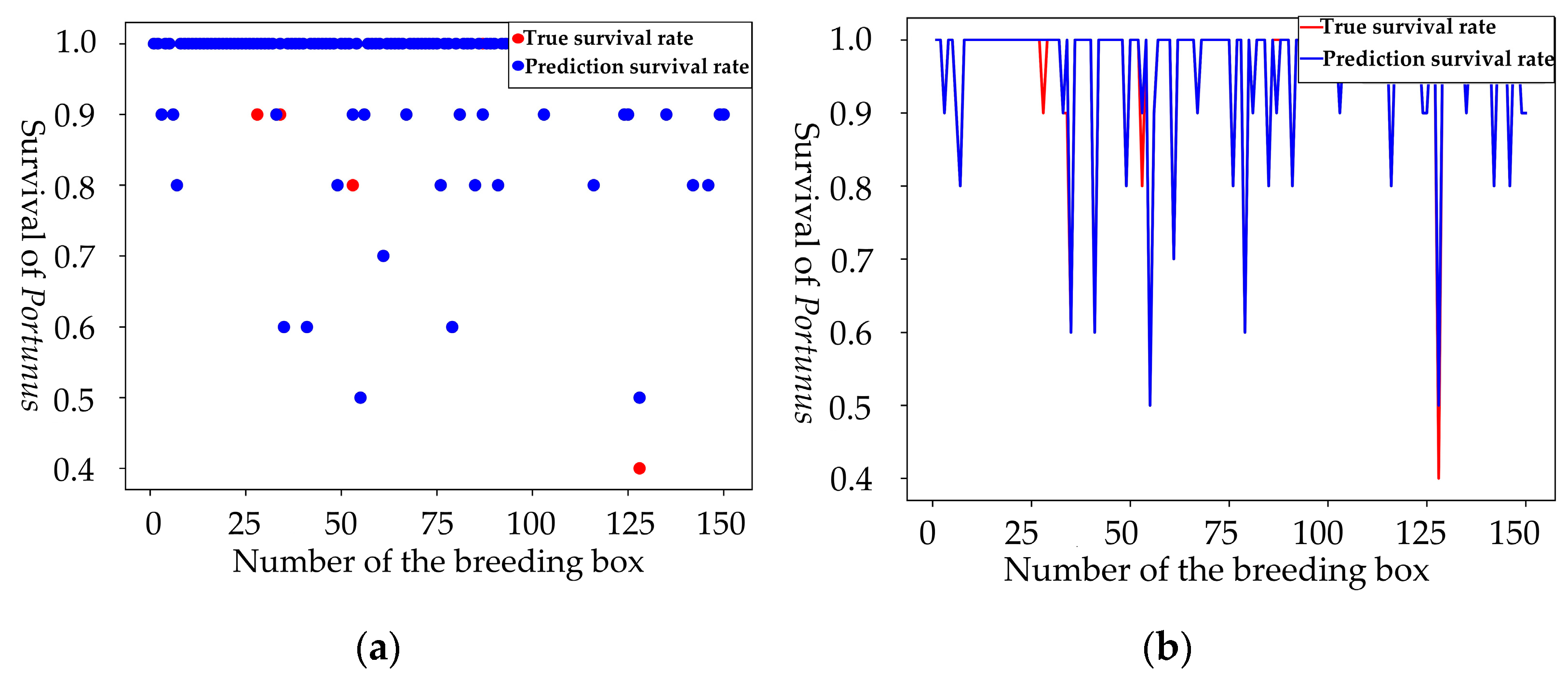
First, based on YOLOV5, RCN, and LWLR networks, the survival rates model of three different characteristic parameters were obtained, respectively. Second, the grid is split into $\left\{1.10,1.20,1.30,1.40\right\}$ for $\partial$ fetching values, as illustrated in

Table 7. Accuracy rates under different ∂ thresholds.

Parameter	Data
∂	1.10	1.20	1.30	1.40
Accuracy	0.960	0.947	0.893	0.920

. Through extracting 350 and 150 image data of 500 sample datasets for training and testing, the paper conducts the fusion judgment. The experimental findings revealed that combining three feature characteristics had the maximum accuracy in predicting Portunus survival at ∂ = 1.10. Figure 16 shows that the multi-parameter fusion predicted values (blue curve) nearly cover the real values (red curve). Moreover, the prediction result of multi-feature parameter fusion is better to that of single feature parameter, with the greatest prediction accuracy of 96.0%.

4. Discussion

Based on the inspection demand of Portunus single-frame three-dimensional aquaculture, a multi-parameter fusion judging model of Portunus survival rate based on machine vision was studied in this paper. Firstly, based on YOLOV5 and the RCN algorithm, the characteristic parameters such as centroid moving distance, residual bait ratio, and rotation angle were obtained. Secondly, based on the LWLR and $soft\mathit{max}$ algorithm, the survival rate regression prediction of Portunus was finally obtained.

5. Conclusions

To detect Portunus survival in real time, the original YOLOV5 and RCN networks missed detection of both pellet feed and contour, and the original algorithm must be optimized and fused with many parameters. Firstly, the k-means clustering algorithm was used to cluster the size of anchors in YOLOV5, which could improve the accuracy of the algorithm model. Through EIOU loss, the convergence was accelerated, and the regression accuracy was also improved. Based on the original basis, the mAP(0.5) values for pellet feed, fish, and shrimp increased by 1.7% and 1%, respectively; EIOU loss increased precision by 2% and mAP (threshold for 0.5:0.95:0.05) by 1.8%; and the prediction accuracy of centroid moving distance and residual bait ratio of Portunus was improved. Secondly, the RCN network was optimized using the double-threshold binary cross-entropy loss function, and its last loss could be reduced to 0.2 when 300 times of training were made. Before optimization, last loss reached 0.23 after 500 training, and the RCN average loss was reduced by 4%. After RCN improvement, the ODS of contour recognition index increases by 2%, the probability of blurring or missing contour prediction was reduced, and the rotation angle of Portunus was obtained. Finally, based on the LWLR and $Logisti{c}_{prediction}$ algorithm, multi-parameter fusion was carried out. The recognition accuracy of the residual bait ratio characteristic parameter to the survival rate of Portunus was 0.920, the recognition accuracy of centroid moving distance characteristic parameter to the survival rate of Portunus was 0.840, the recognition accuracy of rotation angle characteristic parameter to the survival rate of Portunus was 0.955, the recognition accuracy of multi-parameter fusion for the survival rate of Portunus was 0.960, and the accuracy of multi-parameter fusion was 5.5% higher than that of single parameter (average accuracy). Therefore, multi-parameter fusion greatly improves the accuracy of judging whether the Portunus is alive.

References

1. dos Santos, A.M.; Attramadal, K.J.K.; Skogestad, S. Optimal Control of Water Quality in a Recirculating Aquaculture System. IFAC-Pap. OnLine 2022, 55, 328–333. [Google Scholar] [CrossRef]
2. Nguyen, T.-H.; Nguyen, T.-N.; Ngo, B.-V. A VGG-19 Model with Transfer Learning and Image Segmentation for Classification of Tomato Leaf Disease. Agri. Eng. 2022, 4, 871–887. [Google Scholar] [CrossRef]
3. Worasawate, D.; Sakunasinha, P.; Chiangga, S. Automatic Classification of the Ripeness Stage of Mango Fruit Using a Machine Learning Approach. Agric. Eng. 2022, 4, 32–47. [Google Scholar] [CrossRef]
4. Li, X.; Hao, Y.; Zhang, P.; Akhter, M.; Li, D. A novel automatic detection method for abnormal behavior of single fish using image fusion. Comput. Electron. Agric. 2022, 203, 107435. [Google Scholar] [CrossRef]
5. Zheng, K.; Yang, R.; Li, R.; Guo, P.; Yang, L.; Qin, H. A spatiotemporal attention network-based analysis of golden pompano school feeding behavior in an aquaculture vessel. Comput. Electron. Agric. 2023, 205, 107610. [Google Scholar] [CrossRef]
6. Chahid, A.; N’Doye, I.; Majoris, J.E.; Berumen, M.L.; Laleg-Kirati, T.M. Model predictive control paradigms for fish growth reference tracking in precision aquaculture. J. Process Control. 2021, 105, 160–168. [Google Scholar] [CrossRef]
7. Pautsina, A.; Císař, P.; Štys, D.; Terjesen, B.F.; Espmark, Å.M.O. Infrared reflection system for indoor 3D tracking of fish. Aquac. Eng. 2015, 69, 7–17. [Google Scholar] [CrossRef]
8. Duarte, S.; Reig, L.; Oca, J. Measurement of sole activity by digital image analysis. Aquac. Eng. 2009, 41, 22–27. [Google Scholar] [CrossRef]
9. Ye, Z.; Jian, Z.; Han, Z.; Zhu, S.; Li, J.; Lu, H. Behavioral characteristics and statistics-based imaging techniques in the assessment and optimization of tilapia feeding in a recirculating aquaculture system. Trans. ASABE 2016, 59, 345–355. [Google Scholar]
10. Rauf, H.T.; Lali, M.I.U.; Zahoor, S.; Shah, S.Z.H.; Rehman, A.U.; Bukhari, S.A.C. Visual features based automated identification of fish species using deep convolutional neural networks. Comput. Electron. Agric. 2019, 167, 105075. [Google Scholar] [CrossRef]
11. Simonyan, K.; Zisserman, A. Very Deep Convolutional Networks for Large-Scale Image Recognition. arXiv 2014, arXiv:1409.1556. [Google Scholar]
12. Måløy, H.; Aamodt, A.; Misimi, E. A spatio-temporal recurrent network for salmon feeding action recognition from underwater videos in aquaculture. Comput. Electron. Agric. 2019, 167, 105087. [Google Scholar] [CrossRef]
13. Ren, S.; He, K.; Girshick, R.; Sun, J. Faster R-CNN: Towards Real-Time Object Detection with Region Proposal Networks. Adv. Neural Inf. Process. Syst. 2015, 28. [Google Scholar] [CrossRef]
14. Redmon, J.; Divvala, S.; Girshick, R.; Farhadi, A. You Only Look Once: Unified, Real-Time Object Detection. In Proceedings of the IEEE Conference on Computer Vision and Pattern Recognition, Boston, MA, USA, 7–12 June 2015. [Google Scholar]
15. Tang, C.; Zhang, G.; Hu, H.; Wei, P.; Duan, Z.; Qian, Y. An improved YOLOv3 algorithm to detect molting in swimming crabs against a complex background. Aquac. Eng. 2020, 91, 102115. [Google Scholar] [CrossRef]
16. Zeng, L.; Sun, B.; Zhu, D. Underwater target detection based on Faster R-CNN and adversarial occlusion network. Eng. Appl. Artif. Intell. 2021, 100, 104190. [Google Scholar] [CrossRef]
17. Yang, X.; Zhang, S.; Liu, J.; Gao, Q.; Dong, S.; Zhou, C. Deep learning for smart fish farming: Applications, opportunities and challenges. Rev. Aquac. 2021, 38, 6. [Google Scholar] [CrossRef]
18. Li, X.; Shang, M.; Hao, J.; Yang, Z. Accelerating fish detection and recognition by sharing CNNs with objectness learning. In Proceedings of the OCEANS 2016—Shanghai, Shanghai, China, 10–13 April 2016; pp. 1–5. [Google Scholar]
19. Xu, W.; Matzner, S. Underwater Fish Detection Using Deep Learning for Water Power Applications. In Proceedings of the International Conference on Computational Science and Computational Intelligence (CSCI), Las Vegas, NV, USA, 12–14 December 2018; pp. 313–318. [Google Scholar]
20. Redmon, J.; Farhadi, A. Yolov3: An incremental improvement. arXiv e-prints 2018, arXiv:1804.02767. [Google Scholar]
21. Cai, K.; Miao, X.; Wang, W.; Pang, H.; Liu, Y.; Song, J. A modified YOLOv3 model for fish detection based on MobileNetv1 as backbone. Aquac. Eng. 2020, 91, 102117. [Google Scholar] [CrossRef]
22. Xie, S.; Tu, Z. Holistically-Nested Edge Detection. In Proceedings of the IEEE International Conference on Computer Vision (ICCV), Santiago, Chile, 7–13 December 2015; pp. 1395–1403. [Google Scholar]
23. Maninis, K.K.; Pont-Tuset, J.; Arbeláez, P.; Gool, L.V. Convolutional Oriented Boundaries. In Proceedings of the Computer Vision—ECCV, Amsterdam, The Netherlands, 11–14 October 2016; pp. 580–596. [Google Scholar]
24. Badrinarayanan, V.; Kendall, A.; Cipolla, R. SegNet: A Deep Convolutional Encoder-Decoder Architecture for Image Segmentation. arXiv 2015, arXiv:1505.07293. [Google Scholar] [CrossRef]
25. Yang, J.; Price, B.; Cohen, S.; Lee, H.; Yang, M.H. Object Contour Detection with a Fully Convolutional Encoder-Decoder Network. In Proceedings of the IEEE Conference on Computer Vision and Pattern Recognition (CVPR), Las Vegas, NV, USA, 27–30 June 2016; pp. 193–202. [Google Scholar]
26. He, K.; Zhang, X.; Ren, S.; Sun, J. Deep Residual Learning for Image Recognition. In Proceedings of the IEEE Conference on Computer Vision and Pattern Recognition (CVPR), Las Vegas, NV, USA, 27–30 June 2016; pp. 770–778. [Google Scholar]
27. Kelm, A.P.; Rao, V.S.; Zoelzer, U. Object contour and edge detection with refinecontournet. In Proceedings of the Computer Analysis of Images and Patterns, Salerno, Italy, 3–5 September 2019; pp. 246–258. [Google Scholar]
28. Abdennour, N.; Ouni, T.; Amor, N.B. Driver identification using only the CAN-Bus vehicle data through an RCN deep learning approach. Robot. Auton. Syst. 2021, 136, 103707. [Google Scholar] [CrossRef]
29. Zhang, Y.F.; Ren, W.; Zhang, Z.; Jia, Z.; Wang, L.; Tan, T. Focal and efficient iou loss for accurate bounding box regression. Neurocomputing 2021, 506, 146–157. [Google Scholar] [CrossRef]
30. Yu, J.; Jiang, Y.; Wang, Z.; Cao, Z.; Huang, T. Unitbox: An advanced object detection network. In Proceedings of the 24th ACM international conference on Multimedia, Amsterdam, The Netherlands, 15–19 October 2016. [Google Scholar]
31. Rezatofighi, H.; Tsoi, N.; Gwak, J.Y.; Sadeghian, A.; Reid, I.; Savarese, S. Generalized intersection over union: A metric and a loss for bounding box regression. In Proceedings of the IEEE/CVF Conference on Computer Vision and Pattern Recognition, Long Beach, CA, USA, 16–17 June 2019. [Google Scholar]
32. Zheng, Z.; Wang, P.; Liu, W.; Li, J.; Ye, R.; Ren, D. Distance-Iou loss: Faster and better learning for bounding box regression. In Proceedings of the AAAI Conference on Artificial Intelligence, Virtually, 22 February–1 March 2020. [Google Scholar]
Figure 1. (a,b) Portunus in the single-frame three-dimensional breeding frame.
Agriengineering 05 00046 g001
Figure 2. (a) YOLOV5 is the result of the 3-parameter training data. (b) The original YOLOV5 algorithm has missed detection of pellet feed targets.
Agriengineering 05 00046 g002
Figure 3. (a) Comparison of test and training sets of RCN algorithm in loss function based on 300 training sets. (b) Contour target detection with missed contour detection.
Agriengineering 05 00046 g003
Figure 4. (a) The framework flow diagram of YOLOV5. (b) The framework flow diagram of RCN.
Agriengineering 05 00046 g004
Figure 5. (a) The position of the cusp of the crab shell was determined. (b) The coordinates of the cusp were determined. (c) The angle using coordinates A and B were determined.
Agriengineering 05 00046 g005
Figure 6. Framework flow chart for predicting the survival rate of Portunus based on YOLOV5, RCN, and LWLR algorithms.
Agriengineering 05 00046 g006
Figure 7. (a) The calculation frame diagram of DIOU loss. (b) The calculation frame diagram of CIOU loss. (c) The calculation frame diagram of EIOU loss. (d) The training process for predict_boxs in CIOU, and the training process for predict_boxs in EIOU.
Agriengineering 05 00046 g007
Figure 8. (ac) Respectively represent {a,b} under the condition of {0.99,0.95}, {c,d} = {0.6,0.4}, {c,d} = {0.7,0.3}, {c,d} = {0.8,0.2} training set, test set loss curve. (df) Respectively represent {a,b} under the condition of {0.98,0.94}, {c,d} = {0.6,0.4}, {c,d} = {0.7,0.3}, {c,d} = {0.8,0.2} training set, test set loss curve. (gi) Respectively represent {a,b} under the condition of {0.97,0.93}, {c,d} = {0.6,0.4}, {c,d} = {0.7,0.3}, {c,d} = {0.8,0.2} training set, test set loss curve.
Agriengineering 05 00046 g008
Figure 9. (ac) Represent centroid movement distance, residual bait ratio, rotation angle SSE training, and validation curves, respectively. (df) Represent centroid movement distance predicting survival models (k = 0.3), the residual bait ratio predicts the survival rate model (k = 0.02), and rotation angle predicts survival model (k = 1.1), respectively.
Agriengineering 05 00046 g009
Figure 10. (a) Portunus, pellet bait, fish, and shrimp part of the picture dataset. (b) Labeled target detection dataset display.
Agriengineering 05 00046 g010
Figure 11. (a) Euclidean distance method to calculate clustering. (b) 1-IOU distance method to calculate clustering.
Agriengineering 05 00046 g011
Figure 12. (a) Optimized YOLOV5 is the result of the 3-parameter training data. (b) Targeted monitoring of Portunus and residual baits.
Agriengineering 05 00046 g012
Figure 13. (a) Portunus partial data set. (b) Portunus contour partial data set.
Agriengineering 05 00046 g013
Figure 14. Contour detection of Portunus.
Agriengineering 05 00046 g014
Figure 15. (a1,a2) Survival under the feature of centroid moving distance parameter. (b1,b2) Survival rate under the parameter of residual bait ratio. (c1,c2) Survival rate under rotation angle parameter feature.
Agriengineering 05 00046 g015
Figure 16. (a,b) Prediction of survival rate using fusion of feature parameters of centroid moving distance, residual bait ratio, and rotation angle.
Agriengineering 05 00046 g016