Detection and Localization of the FDI Attacks in the Presence of DoS Attacks in Smart Grid

Highlights

What are the main findings?

• The L2 norm of Forecasting error can be used to effectively define a threshold and detect the FDIA.
• Simultaneous DoS and FDIA attacks degrade the accuracy of multi-label localization models.

What is the implication of the main finding?

• The hybrid parallel CNN and sequential Transformer-BiLSTM architecture provides high-accuracy forecasts of power system behavior.
• The use of forecast error as an input enables accurate FDIA localization despite partial sensor unavailability caused by DoS attacks.
• The proposed framework demonstrates resilience in real-time smart grid monitoring, enabling early detection and localization of cyberattacks despite sensor-level disruptions.

Abstract

Smart grids (SGs) are becoming increasingly complex with the integration of communication, protection, and automation technologies. However, this digital transformation has introduced new vulnerabilities, especially false data injection attacks (FDIAs) and Denial of Service (DoS) attacks. FDIAs can subtly corrupt measurement data, misleading operators without triggering traditional bad data detection (BDD) methods in state estimation (SE), while DoS attacks disrupt the availability of sensor data, affecting grid observability. This paper presents a deep learning-based framework for detecting and localizing FDIAs, including under DoS conditions. A hybrid CNN, Transformer, and BiLSTM model captures spatial, global, and temporal correlations to forecast measurements and detect anomalies using a threshold-based approach. For further detection and localization, a Multi-layer Perceptron (MLP) model maps forecast errors to the compromised sensor locations, effectively complementing or replacing BDD methods. Unlike conventional SE, the approach is fully data-driven and does not require knowledge of grid topology. Experimental evaluation on IEEE 14–bus and 118–bus systems demonstrates strong performance for the FDIA condition, including precision of 0.9985, recall of 0.9980, and row-wise accuracy (RACC) of 0.9670 under simultaneous FDIA and DoS conditions. Furthermore, the proposed method outperforms existing machine learning models, showcasing its potential for real-time cybersecurity and situational awareness in modern SGs.

1. Introduction

The transition from conventional power grids to smart grids, often referred to as the next generation of the power grid, has been driven by the integration of Information and Communication Technologies (ICTs) [1]. This evolution has fostered an automated energy delivery network with bidirectional energy and information flow, distributed generation, self-healing, and pervasive control [2]. The bidirectional information flow has led to the availability of big data in SG. Although it has nurtured real-time monitoring of the SG through Supervisory Control and Data Acquisition (SCADA) systems, increasing the reliability and efficiency of the grid, it has made the SG vulnerable to various cyber threats. SCADA periodically scans the voltage, active power, reactive power, and system topology at a rate of 2 to 10 s to monitor the SG [3]. These measurements are also fed to the state estimator for state estimation (SE), which estimates the unknown state variable in SG. Estimated states play a vital role in various Energy Management System (EMS) applications, such as optimal power flow, economic dispatch, and security assessment [4]. The state estimator also includes the bad-data detector, which acts as a defense layer against cyberattacks. Despite these protections, the SG remains susceptible to multiple classes of cyberattacks, particularly those that compromise data integrity and availability, such as False Data Injection Attacks (FDIAs) and Denial of Service (DoS) attacks.

In recent years, several cyberattacks have reportedly targeted the smart grid [5]. As the energy sector is a critical infrastructure, disruption of SG operations has severe economic consequences. In the worst case, it can initiate a chain of events that results in the grid’s collapse. Cyberattacks in SG generally fall into three main categories: component-wise attacks, which target individual devices or systems; protocol-wise attacks, which exploit vulnerabilities in communication protocols; and topology-wise attacks, which exploit vulnerabilities in network topology [6]. FDIA is a prevalent and serious cybersecurity threat in SG [7]. FDIA aims to compromise the state estimation of SG by introducing malicious data into meter readings. Although BDD immediately detects a random and uncoordinated data injection attack, carefully crafting the injected measurements can bypass the conventional BDD of SE [8,9]. The attacker can perform FDIA and bypass BDD by modifying the values of a small set of sensors with limited knowledge of the grid topology [10]. This stealthy FDIA results in incorrect state prediction and leads to the imbalance of generation and load, ultimately causing a system to collapse. On the other hand, DoS attacks disrupt the availability of sensor measurement, leading to partial observability of the grid [11]. When launched in tandem with FDIAs, DoS attacks reduce redundancy in the measurement set, making it more challenging to detect stealthy data manipulation.

FDIA poses a significant threat to SG, and its detection and mitigation have been the focus of substantial research studies. FDIA detection approaches can be grouped primarily into model-based and data-driven approaches. The model-based approach requires the complete topological information and mathematical formulation to estimate the states for BDD. In [12], the author developed a Euclidean detector and Kalman filter estimator for FDIA. A chi-square test was suggested in [13] for FDIA detection. Although model-based approaches offer real-time FDIA detection with less computational burden, their dependencies on precise mathematical formulation cause various uncertainties and disturbances [14]. Recently, data-driven approaches have gained traction in the detection of FDIA due to their lack of dependency on system topology information. The data-driven approach learns from historical measurements and employs the classification- or threshold-based approach to detect FDIA [15]. In addition to FDIA detection, the localization of the FDIA attack is instrumental in quickly isolating the compromised sensor and ensuring grid stability and reliability. Various studies have followed the multilabel classification approach to accurately predict FDIA locations [16].

In this paper, an online FDIA detection is proposed using a hybrid model that combines Convolutional Neural Networks (CNN), Transformer (Tr), and Bidirectional Long Short Term Memory (BiLSTM). Unlike a conventional sequential architecture, the proposed model processes the input in parallel by feeding the data into separate CNN and sequential Tr-BiLSTM blocks, leveraging their strengths in handling temporal patterns, global contextual understanding, and sequential dependencies. The parallel hybrid CNN and Tr-BiLSTM is used to forecast the measurements of the next timestep by learning from a historical dataset. An appropriate threshold is carefully chosen to detect the presence of FDIA. Moreover, a Multilayer Perceptron (MLP) or Random Forest (RF) is used to detect the location of the FDIA-poisoned sensors by training on the error between the forecasted and actual measurements. The proposed framework is also extended to operate under DoS scenarios to allow continued operation of the localization module. Our main contributions are as follows.

• A novel data-driven CNN, Transformer, and BiLSTM-based model is introduced in conjunction with MLP to detect and localize FDIA attacks in SG. To the best of our knowledge, this study is the first to use the proposed architecture in this particular research field.
• The proposed approach is universally applicable and does not rely on statistical assumptions about the system parameters and attack model.
• The comparative analysis of our proposed model and other existing models for FDIA detection and localization, reported in various literature, is performed to showcase the effectiveness of our proposed model in the IEEE 14–bus and IEEE 118–bus test systems.
• The framework is evaluated under standard FDIA conditions and scenarios in which FDIA is combined with DoS attacks, demonstrating its robustness under partial observability. This work is among the few studies that jointly investigate the impact of FDIA and DoS in a unified detection and localization framework.

The remainder of the article is organized as follows. Section 2 provides a comprehensive review of the existing literature. The preliminary information is discussed in detail in Section 3. The framework and architecture of the proposed model are presented in Section 4. The performance of the proposed approach for various scenarios is described in Section 5. Finally, the paper is concluded in Section 6.

2. Related Works

Recent advancements in artificial intelligence have encouraged the adoption of various machine learning (ML) and deep learning (DL) techniques to estimate the state, detect, and localize FDIA. This section contains a brief summary of the related works. The authors in [17] investigated the viability of the Feed Forward Neural Networks (FFNNs) and LSTM to estimate the state of the IEEE 14–bus and IEEE 118–bus. The author concluded that the LSTM is superior to FFNNs, WLS, and WLAV against FDIA-poisoned data. A stacked ResNetD method was proposed as an alternative to the state estimator in [18]. The stacked ResNetD outperformed the MLP, CNN, and ProlNet DL techniques to predict the states of the various IEEE benchmarks. In [19], the author proposed exponential GPR over medium Gaussian SVM and fine Gaussian SVM for state estimation using data-driven techniques. However, these studies lacked the implementation of BDD to detect FDIA. In [20], the principal component analysis (PCA) is used to set the optimal threshold of $2.98\times {10}^{-5}$ to detect the FDIA in the IEEE 118–bus. They reported that PCA is better at detecting BDD than SVM. The authors in [21] concluded that the Stacked Auto Encoder (SAE) was superior to SVM by detecting the 11 anomaly states in contrast to the six anomaly states in several IEEE benchmarks. Although the above approaches are superior to the support vector machine (SVM) technique, their performance is not compared with various DL models. In [22], the author has utilized the hybrid Transformer and LSTM-based architecture to detect and localize the FDIA for hourly and minute data from the IEEE 14–bus system. The proposed model uses the threshold to detect FDIA, but it suffers from the problem of low RACC. The author proposed a Maximum A Posteriori (MAP) approach using sparsity priors to estimate the attack vector, and the likelihood of the data being normal or under FDIA is modeled using a Gaussian Mixture Model (GMM) in [23]. However, this algorithm is iterative and alternates between MAP and GMM steps in an Expectation-Maximization-like fashion for localization, which is computationally burdensome. In [24], the authors employed federated learning to distinguish between normal and attack scenarios, concluding that BiLSTM and Bi-GRU with attention achieved the best results. However, centralized versions of these attention-based models were not evaluated, leaving a gap in the comparative analysis. Although federated learning enhances privacy, the study showed that the centralized LSTM and GRU models outperformed their federated counterparts. Similarly, ref. [25] explored a vertical federated learning approach for FDIA detection. Despite its benefits in privacy protection, this method solely focuses on detection and introduces additional complexity and reduced accuracy compared to centralized learning approaches. The study in [26] introduced a Hodge Graph Neural Network (HodgeGNN) for FDIA localization, leveraging edge-space representations to model spatial dependencies in the grid. However, the reliance on a specific graph structure may reduce its application across varying grid configurations. In [27], the authors proposed an ensemble of CNN models combined with Explainable Artificial Intelligence (XAI) for FDIA detection and localization in distribution systems. While their method achieved high accuracy, the lack of temporal modeling limits its performance in capturing time-series dependencies. In [28], a dimensionality reduction strategy based on Local Outlier Standard Score Analysis (LOSSA) was integrated with an AdaBoost decision tree for FDIA detection. Although this approach enhances detection efficiency, it does not provide localization, which restricts its utility for situational awareness and response strategies.

In the last decade, the localization of FDIA has been framed as a multilabel classification problem. The multilabel classification approach enables each feature to have its own binary or categorical labels, where each label is independent. One of the first works includes multilabel classification using CNN [16]. A CNN-based FDIA location detection algorithm was proposed as a complementary technology to BDD, compared to MLP and LightGBM. The author concluded that CNN is more accurate and scalable by comparing its performance in the IEEE 14 and IEEE 118–buses. In [29], the author reinforced the superior performance of CNN, but concluded that the Exiting Mechanism and Mixed-Precision Quantization (EE-MPQ) is time efficient for the evaluation of the IEEE 14 and 118 bus systems. The author proposed a hybrid SVM and CNN-based architecture [27], where SVM merges the spatio-temporal CNN output. They applied Gradient-weighted Class Activation mapping (Grad-CAM) for better localization and interpretability. However, they pointed out its drawbacks in detecting new zero-day attacks. In [30], the author proposed a spatio-temporal sequence analysis by combining the outputs of the Gated Temporal Convolutional Network (GTCN) and the GCN to localize the attack in a grid rich in Renewable Energy (RE). The author investigated the spectral Graphical Neural Network (GNN) using Auto-Regressive Moving Average (ARMA) filters to locate the FDIA across IEEE 57-, 118-, and 300-bus systems [31]. The author in [32] proposed the Recursive Variational Graph Autoencoder (ReVGAE), which uses a Graph Convolutional Network (GCN) as an encoder and decoder to reconstruct data and topology, and denoising. The evaluation of ReVGAE on the IEEE 14–bus generated the ROC-AUC curve of 0.9667. In [33], FDIA is localized by constructing a causality graph assuming that FDIA disrupts the expected causal links. A Graph Attention Network learns attention-weighted node embeddings to highlight suspicious measurements, but this method is very sensitive to noise and non-stationary conditions. In the aforementioned algorithms, topology information was the prerequisite to locate the attacks.

In addition to standalone FDIA, some recent studies have investigated the combined impact of DoS and FDIA, representing a more realistic and dangerous threat model in smart grids. These hybrid attacks aim to degrade the observability of the system by blocking sensor data and simultaneously injecting malicious measurements and confusing detection mechanisms. The authors in [34] proposed a sliding mode observer to co-estimate states and FDI attacks in multi-area load frequency control systems, where they introduced an attack compensation controller to mitigate hybrid attack impacts. Similarly, the study in [35] designed a resilient observer-based controller for stochastic systems to maintain performance under coordinated DoS and FDIA attacks using a Markov jump framework. In the context of DC microgrids, ref. [36] presented a fuzzy switching-type estimator and compensator, while ref. [37] incorporated event-triggered mechanisms to minimize communication overhead during hybrid attack mitigation. In [38], a distributed approach was used to jointly estimate the states of the system and attacks, using multiple adversarial strategies. Despite their strengths, most of these methods focus on either control, with limited work tackling the detection and localization of FDIA during DoS-induced observability loss. In [39], the authors employed an attention-enhanced Temporal Convolutional Denoising Autoencoder (TCDAE) combined with an MLP to detect and reconstruct FDIA under combined DoS and FDIA conditions. In contrast, ref. [40] proposed a graph-based TCDAE model to handle missing data, identify network topology, and localize FDIA simultaneously. Both works focus on distributed networks, and they did not explicitly consider Row Accuracy (RACC), which is critical for evaluating localization reliability in multilabel settings, as a model may exhibit high overall accuracy despite poor localization performance. This broader gap is addressed by our proposed CNN–Tr-BiLSTM–RF framework, which is tailored for transmission networks and explicitly accounts for key performance metrics such as RACC, allowing robust and scalable FDIA detection and localization during limited sensor visibility.

In SG, the measurement of each sensor exhibits spatial, global, and temporal correlations due to the interdependence among sensors and the time-varying nature of load dynamics. While CNN effectively captures spatial patterns and local dependencies across correlated measurements, BiLSTM networks are more suitable for capturing temporal dependencies, and Transformer enhances the model’s ability to capture global contextual relationships across the sequence. By training on historical data, the CNN, Transformer, and BiLSTM hybrid model leverages spatial, global, and temporal features, enabling robust detection and localization of stealthy FDIAs under complete and partial observability, as demonstrated by our experimental results.

3. Preliminaries

3.1. State Estimation

SE is the process of determining the unknown states of the grids from known variables or measurements collected from existing sensors [41]. SE can be framed as an unconstrained optimization problem, where the power flow equations are used to relate the measurement vector [42]. SG can be analyzed using either AC power or DC power flow analysis. In an AC power flow analysis, the magnitude and angles of voltage and/or currents are used, as opposed to the DC power flow analysis, where the voltage magnitude is assumed to be constant and only the voltage phase angles of the buses are considered [43]. AC power flow analysis is a more accurate representation of today’s SG, but it is computationally heavy and raises the issue of nonlinearity [22]. In contrast, DC power flow analysis is simple and commonly used for real-time operations, so we have considered the DC linearized state estimation method for power flow analysis with $n+1$ buses and t transmission lines. Equation (1) shows the relationship between the state vector and the measurement vector.

$$z=h\left(x\right)+e$$

(1)

where $z=\{z_1,\dots ,z_m\}\in {\mathbb{R}}^m$ is the measurement vector, $x=\{x_1,\dots ,x_n\}\in {\mathbb{R}}^n$ is the state vector, $h\left(x\right)=\{h_1\left(x\right),\dots ,h_m\left(k\right)\}$ is the non-linear measurement function that relates the state and the measurement vector, and e is the Gaussian noise of shape $m\times 1$. For the linearized DC power flow assumption, the equation modifies to:

$$z=Hx+e$$

(2)

where $H\in {\mathbb{R}}^{m\times n}$ represents the Jacobian matrix and $m\ge n$. The solution to Equation (2) can be found using Equation (3).

$$\widehat{x}={\left(H^{T}WH\right)}^{-1}{H}^{T}Wz$$

(3)

where $\widehat{x}$ is the state vector when e has a zero mean distribution, and W is the diagonal matrix. For the zero-mean distribution of e, $\widehat{z}=h\left(\widehat{x}\right)$ is the measurement estimate. The conventional SE detects malicious data injection with the help of BDD techniques. In a BDD, the residual (R) between the state estimates and the observed measurement vector is compared with predefined thresholds $\tau$ to determine bad data, as shown in Equation (4).

$$R=∥z-h\left(\widehat{x}\right)∥\ge \tau$$

(4)

Bad data occurs mainly due to measurement errors such as meter biases, faulty connections, incorrect topology information, and unforeseen noise [44]. These errors do not follow an expected Gaussian distribution, generating a larger error than the threshold, which BDD immediately flags.

3.2. False Data Injection Attack

FDIA is designed to bypass BDD by adding erroneous data to actual measurements, resulting in a change in the state variable of the system [45]. If a is the injected measurement such that $a=Hc$ where $c\ne 0\in {\mathbb{R}}^n$, the observed measurement vector is denoted by Equation (5).

$$\widehat{z}=z+a$$

(5)

The stealthy FDIA occurs if the residual of the modified measurement vectors is equal to the residual of the original measurement vectors, as shown in Equation (6). For stealthy FDIA, the attacker can craft the injected measurement with complete or partial knowledge of the H matrix using min-cut methods [46].

$$∥\widehat{z}-H\widehat{x}∥=∥z+a-H(x+c)∥=∥z-Hx∥$$

(6)

3.3. DoS

A DoS attack disrupts the availability of the sensor measurements by overwhelming or blocking access to the sensor. The DoS attack can be induced by network flooding, jamming attacks, protocol exploitation, and physical isolation of sensors. Let ${\mathbf{x}}_t\in {\mathbb{R}}^d$ represent the system’s measurement vector at time t, where N is the total number of sensors. A binary mask vector $\mathbf{m}\in {\{0,1\}}^N$ is defined such that:

$$m^{\left(i\right)}=\left\{\begin{array}{cc}1,\hfill & \mathrm{if}\mathrm{sensor}i\mathrm{is}\mathrm{not}\mathrm{under}\mathrm{DoS}\mathrm{attack},\hfill \\ 0,\hfill & \mathrm{if}\mathrm{sensor}i\mathrm{is}\mathrm{under}\mathrm{DoS}\mathrm{attack}\hfill \end{array}\right.$$

(7)

The observed measurement vector in the presence of a DoS attack is given by:

$$\tilde{\mathbf{x}}=\mathbf{m}\odot \mathbf{x},$$

(8)

where ⊙ denotes element-wise multiplication. The binary mask $\mathbf{m}\in {\{0,1\}}^d$ effectively zeros out the measurements from the sensors under attack, simulating the effect of a DoS event.

3.4. CNN

CNN was initially proposed for large-scale image processing [47], but has proven effective for processing sequential data, such as time series signals in power systems. 1D CNN applies convolutional filters across timesteps to extract localized temporal features. The operation in the first convolutional layer is defined as [16]:

$$c_{1,j}=\mathrm{ReLU}(z\ast h_{1,j}+b_{1,j})$$

(9)

where $c_{1,j}$ is the output feature map of the first convolutional layer, z is the multivariate input sequence, $h_{1,j}$ is the j-th kernel, and $b_{1,j}$ is the bias added to the output, ∗ represents the convolution operation, and the Rectified Linear Unit (ReLU) is the activation function. The output after the Pth convolutional layer is as follows.

$$c_{P,j}=\mathrm{ReLU}(c_{P-1,j}\ast h_{1,j}+b_{1,j})$$

(10)

Batch normalization is applied after each convolution to normalize activations and accelerate training. Global average pooling reduces each feature map to a single value, preserving important patterns while mitigating overfitting. The CNN architecture is depicted in Figure 1.

3.5. BiLSTM

Recurrent Neural Networks (RNNs) often suffer from the problem of vanishing gradients, which affects the learning of long-term dependencies. LSTM networks address this by incorporating gating mechanisms to retain relevant information across time steps [48]. BiLSTM extends LSTM by processing sequences in both forward and backward directions, enabling better context capture for multivariate time series data, such as smart grid measurements [49]. At each time step t, the LSTM cell takes the input $x_t$, the previous hidden state $h_{t-1}$, and the previous cell state $c_{t-1}$. The memory cell and hidden state are updated using Equations (11) and (12), respectively [50]:

$$c_t=f_t·c_{t-1}+g_t·i_t$$

(11)

$$h_t=o_t·\beta \left(c_t\right)$$

(12)

Each gate is computed as follows:

$$i_t=\sigma (W_i{x}_t+R_i{h}_{t-1}+b_i)$$

(13)

$$f_t=\sigma (W_f{x}_t+R_f{h}_{t-1}+b_f)$$

(14)

$$g_t=\beta (W_g{x}_t+R_g{h}_{t-1}+b_g)$$

(15)

$$o_t=\sigma (W_o{x}_t+R_o{h}_{t-1}+b_o)$$

(16)

where $i_t$, $f_t$, $g_t$, and $o_t$ are the input gate, the forget gate, the input node, and the output gate, respectively. $W_i$, $W_f$, $W_g$, and $W_o$ denote the weight matrices corresponding to the respective inputs and hidden states of the network’s activation functions. The operator ‘·’ indicates element-wise multiplication. The function $\sigma$ represents the sigmoid activation, while $\beta$ denotes the hyperbolic tangent (tanh) function. The structure of a single LSTM block is shown in Figure 2.

The BiLSTM consists of two independent LSTM layers that process the input sequence in forward and backward directions. The structure of the BiLSTM block is shown in Figure 3.

At each time step t, the forward LSTM computes the hidden state $\overrightarrow{h_t}$ based on the previous forward hidden state $\overrightarrow{h_{t-1}}$ and the current input $x_t$, while the backward LSTM computes the hidden state $\overleftarrow{h_t}$ based on the subsequent backward hidden state $\overleftarrow{h_{t+1}}$ and the same input $x_t$. Although the parameters of the forward and backward LSTM are independent, both directions share the same input embedding sequence, as shown in Equations (17) and (18).

$$\overrightarrow{h_t}={\mathrm{LSTM}}_{\mathrm{fwd}}(x_t,\overrightarrow{h_{t-1}})$$

(17)

$$\overleftarrow{h_t}={\mathrm{LSTM}}_{\mathrm{bwd}}(x_t,\overleftarrow{h_{t+1}})$$

(18)

The final hidden state of the BiLSTM at timestep t is obtained by concatenating the hidden states from both directions, as shown in the equations below.

$$h_t=[\overrightarrow{h_t};\overleftarrow{h_t}]$$

(19)

3.6. Transformer with Multi-Head Attention

The Transformer architecture leverages parallel attention mechanisms to process sequential data without relying on recurrence, enabling it to effectively capture long-range dependencies. The incorporation of multi-head attention further enhances its capacity to model complex temporal relationships across arbitrary time steps, allowing the network to jointly learn both local and global patterns in multivariate sensor data [51]. Given an input sequence $X\in {\mathbb{R}}^{n\times d_{\mathrm{model}}}$, where n is the sequence length and $d_{\mathrm{model}}$ is the feature dimension, linear projections are used to compute the queries Q, keys K, and values V:

$$Q=X{W}^Q,K=X{W}^K,V=X{W}^V$$

(20)

where $W^Q,W^K,W^V\in {\mathbb{R}}^{d_{\mathrm{model}} \times d_k}$ are learnable weight matrices and $d_k$ is the dimension of each attention head. The scaled dot-product attention is computed as:

$$\mathrm{Attention}(Q,K,V)=\mathrm{softmax}\left({\displaystyle \frac{Q{K}^{\top }}{\sqrt{d_k}}}\right)V$$

(21)

In practice, the Transformer uses h attention heads in parallel. Each head computes attention independently:

$${\mathrm{head}}_i=\mathrm{Attention}(Q{W}_i^Q,K{W}_i^K,V{W}_i^V)$$

(22)

The results are concatenated and projected back to $d_{\mathrm{model}}$ dimensions:

$$\mathrm{MultiHead}(Q,K,V)=\mathrm{Concat}({\mathrm{head}}_1,\dots ,{\mathrm{head}}_h)W^O$$

(23)

where $W^O\in {\mathbb{R}}^{h{d}_k \times d_{\mathrm{model}}}$ is another trainable matrix. A residual connection followed by layer normalization is applied to preserve gradient flow:

$$Z=\mathrm{LayerNorm}(X+\mathrm{MultiHead}(Q,K,V\left)\right)$$

(24)

Next, a position-wise feedforward network (FFN) is applied:

$$\mathrm{FFN}\left(z\right)=max(0,z{W}_1+b_1)W_2+b_2$$

(25)

where $W_1\in {\mathbb{R}}^{d_{\mathrm{model}} \times d_{\mathrm{ff}}}$ and $W_2\in {\mathbb{R}}^{d_{\mathrm{ff}} \times d_{\mathrm{model}}}$. A second residual connection and normalization complete the Transformer block:

$$\mathrm{Output}=\mathrm{LayerNorm}(Z+\mathrm{FFN}(Z\left)\right)$$

(26)

3.7. MLP

MLP is a feedforward artificial neural network architecture consisting of an input layer, one or more hidden layers, and an output layer. Each neuron in a layer is fully connected to all neurons in the subsequent layer via trainable weights. Nonlinear transformations are applied using activation functions such as ReLU or sigmoid to map nonlinear relationships. Let the input vector be $x=x_1,x_2,\dots ,x_N$, connected to hidden neurons ${\alpha }_1,\dots ,{\alpha }_H$ and output neurons ${\beta }_1,\dots ,{\beta }_L$. The weights between the input and hidden neurons are denoted $W_{{\alpha }_j{x}_i}$, and between the hidden and the output neurons as $W_{{\beta }_l{\alpha }_j}$. The backpropagation and gradient descent methods update the weights and biases. The transformation at the l-th layer is defined as:

$$h^{\left(l\right)}=\varphi \left(W^{\left(l\right)}{h}^{(l-1)}+b^{\left(l\right)}\right)$$

(27)

where $h^{\left(l\right)}$ is the output of the activation function, $W^{\left(l\right)}$ is the trainable weight matrix, $b^{\left(l\right)}$ is the bias vector, and $\varphi (·)$ is the non-linear activation function.

3.8. RF

Random Forest (RF) is a supervised machine learning technique composed of multiple decision trees $h(x,k)$, each trained on a different bootstrap sample drawn from the dataset [52]. To introduce randomness, only a subset of features $(m<M)$ is considered at each node split, which enhances generalization and reduces overfitting. The division of nodes is based on the Gini impurity [53], defined as:

$$Gini\left(D\right)=1-\sum _{i=1}^m{P}_i^2$$

(28)

$$Gin{i}_s={\displaystyle \frac{|D_1|}{\left|D\right|}}·Gini\left(D_1\right)+\cdots +{\displaystyle \frac{|D_o|}{\left|D\right|}}·Gini\left(D_o\right)$$

(29)

where $Gini\left(D\right)$ is the Gini index before the split, $P_i=d/D$, d is the total sample that exists in the D datasets, $Gin{i}_s$ is the Gini index after the split, and $D_1$ and $D_0$ are the subsets of D. The model grows trees to full depth or until stopping criteria (e.g., minimum samples per leaf) are met. The schematic diagram of the random forest is shown in Figure 4.

4. Methodology

This section provides details on the FDIA detection and localization scheme. In addition, it outlines the proposed hybrid ML architecture.

4.1. Proposed FDIA Detection and Localization Scheme

FDIA detection using ML techniques is commonly framed as a binary classification task, in which the labels can be 0 or 1. An alternative to the binary classification approach is to implement threshold-based detection using ML techniques. In our proposed approach, we train a hybrid ML-based forecasting module on historical measurements offline. The forecasting module is trained only on normal data to forecast the variables for the next time steps, and a threshold is extracted for BDD based on the forecast outputs, as shown in Equation (30).

$$\left|E\right|=\sqrt{e_1^2+e_2^2+\cdots +e_N^2}$$

(30)

where $e_N$ is the error between the Nth forecast variable and the corresponding observed variable. The E represents the Euclidean norm of an error vector between the forecasted and observed variables.

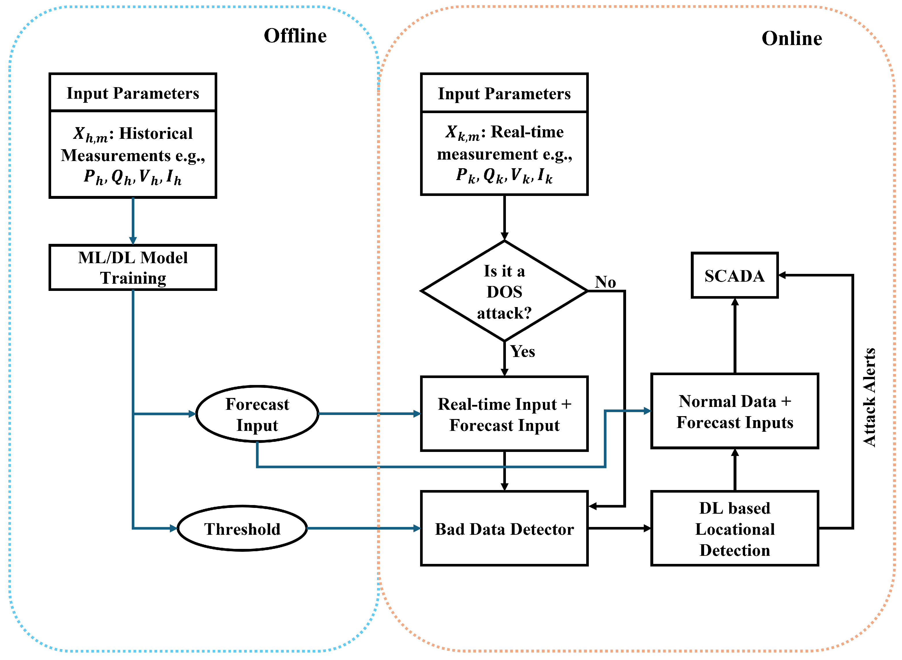
For the detection of FDIA in the first stage, the Euclidean norm of observed variables is compared with the threshold to detect FDIA. The threshold-based approach is used as the first stage of detection and is widely reported in various literature [20,22]. The FDIA localization using ML techniques is framed as a multilabel task. In this approach, each label is independent of the others and can have binary or categorical labels [54]. Multilabel classification is data-driven and does not require any information on grid topology or Jacobian matrix H. In our proposed approach, the error between the forecast and the observed input is fed to another ML classifier to identify whether the variable of each sensor is under attack. In the presence of a DoS attack, the sensor is out of operation and does not report any measurements. In such a scenario, the forecast output is considered as an observed output for the corresponding sensors under attack. The modified variables are fed to the BDD to evaluate the presence of FDIA. In addition, these outputs are fed to the location detection module or multilabel classifier to localize the FDIA. This evaluation of the observed data, regardless of the triggering of BDD, creates redundancy and enhances the detection and localization of the FDIA. In the presence of FDIA, the FDIA alarm, normal variables, and forecast variables are sent to SCADA, allowing the grid operator to make an informed decision. The flow chart of the proposed scheme is shown in Figure 5.

4.2. Proposed ML Architecture

1D-CNN has demonstrated strong performance in time series classification tasks due to its ability to efficiently extract local temporal patterns [55,56]. Similarly, BiLSTM networks are widely used in sequential data modeling, particularly in Natural Language Processing [57] and anomaly detection applications [58,59]. 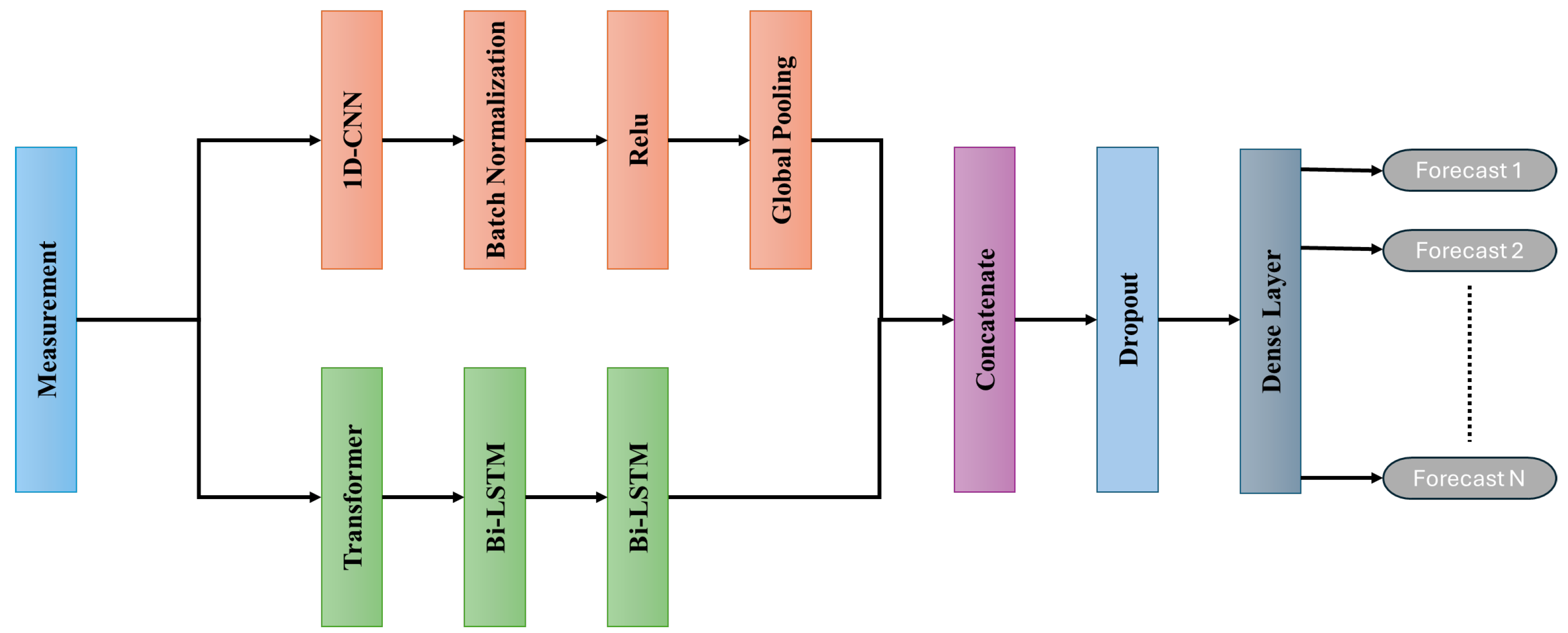Recently, transformer-based architectures have gained attention for their ability to capture short-range and long-range dependencies through attention mechanisms, showing promising results in time-series forecasting without relying on recurrence [60]. The parallel CNN and Tr-BiLSTM architecture proposed for the next-step forecasting is illustrated in Figure 6. It consists of two parallel components: a CNN block that operates independently and a sequential Transformer–BiLSTM block.

The 1D-CNN layer applies convolutional filters across the temporal dimension to extract localized features from the raw input. This is followed by batch normalization and ReLU activation to stabilize and accelerate training while introducing nonlinearity. In parallel, the input is also passed through a Transformer block that captures global temporal dependencies using multi-head self-attention. The output of the Transformer is subsequently processed by stacked BiLSTM layers to model long-range temporal dependencies in both forward and backward directions, enriching the temporal context. The resulting features are aggregated using Global Average Pooling to reduce dimensionality, followed by a dense layer that outputs the forecasted measurements for the next time step.

It is worth noting that while Transformers typically require positional encoding to retain temporal order, this component is omitted in the proposed architecture, as temporal dependencies are captured by the BiLSTM layer. FDIA localization is subsequently performed using an MLP or RF classifier. The input to the MLP or RF is the forecast error, the difference between the predicted and observed sensor measurements. The output is binary, with a value of 0 indicating a normal measurement and 1 indicating the presence of an FDIA.

4.3. Dataset

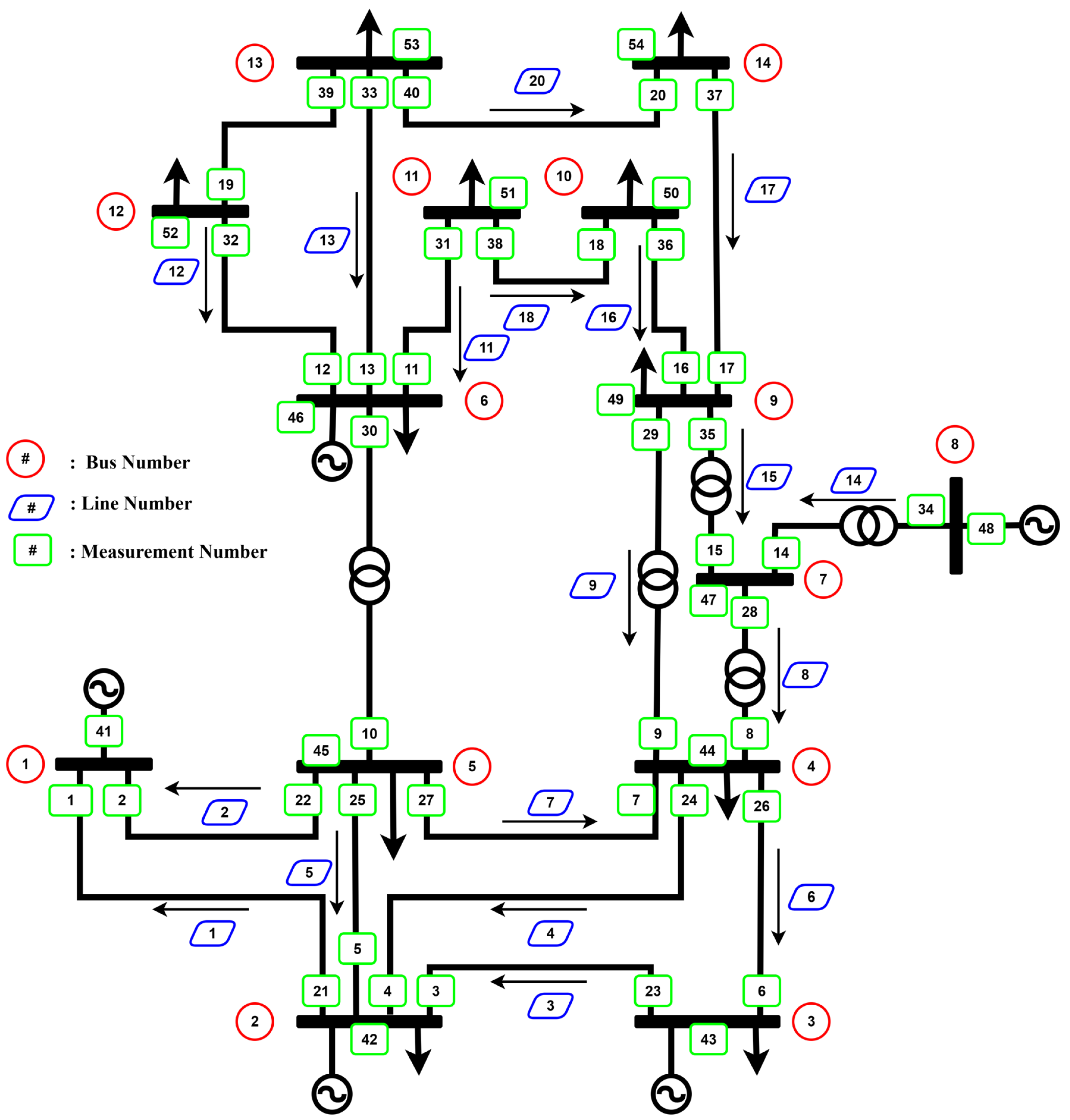
The energy sector is critical infrastructure, and there is little to no publicly available dataset due to privacy and security concerns. The hourly dataset used in this study was taken from [61], and the load profile for the dataset is taken from [62]. The dataset was generated using DC state estimation and made publicly available; however, our proposed framework for detection and localization is also applicable to AC state estimation. The normal dataset consists of 8760 samples along with 54 features for the IEEE 14–bus system. Similarly, the normal dataset of 8760 samples and 490 features was generated using DC state estimation for the IEEE 118–bus as part of this study. Gaussian noise, up to 4% of the true value, was added to the normal measurement to mimic the presence of real-world noise. The IEEE 14–bus dataset comprises 54 features, each corresponding to specific measurements within the IEEE 14–bus system. The initial 20 features capture the forward power flow through the transmission lines, the subsequent 20 reflect the reverse flow on the same lines, and the remaining 14 features represent the power consumption on each of the 14 buses as shown in Figure 7. The IEEE 118–bus dataset comprises 490 features, of which the initial 372 features capture the forward and reverse power flow through the transmission lines, and the 118 features correspond to the power consumption at each of the 118 buses.

This study uses an attack vector dataset originally presented in [63]. The attack vector dataset contains 128 FDIA vectors for the IEEE 14–bus system and 250 FDIA vectors designed for the IEEE 118–bus system, all of which successfully bypass traditional BDD. In addition, the attack vectors in the dataset were further scaled by 3/4, 2/3, and 1/2 to generate more stealthier attacks. For $a=Hc\Rightarrow \gamma a=H\gamma c$ and $a^{\prime }=\gamma a$, where $\gamma \in \mathbb{R}$, is also a valid stealth attack vector. Figure 8 presents the sensor measurements at a randomly selected timestep under different $\gamma$-scaled attack scenarios using the sparsest attack vector.

4.4. Training Procedure

The proposed FDIA detection framework consists of two key modules: a forecasting-based anomaly detection module and a location detection module. The forecasting module uses a hybrid CNN, Transformer, and BiLSTM architecture that exploits spatial, global, and temporal features in multivariate time series measurements from the power grid.

The input in the forecasting module is a sequence of past system measurements over a fixed window of 48 h, denoted by $\mathbf{X}\in {\mathbb{R}}^{48 \times M}$, where M is the total number of sensors. The architecture comprises two parallel branches. The CNN branch applies a one-dimensional convolutional layer with 128 filters, a kernel size of 3, and ‘same’ padding. The output undergoes batch normalization, followed by ReLU activation and global average pooling. In the second branch, the input is passed through a transformer block configured with six attention heads and a key dimension of 9. The attention output is regularized using a dropout rate of 0.1 and combined with the residual input, followed by layer normalization. This is followed by a position-wise FFN with 128 hidden units and ReLU activation, another residual connection, and a second layer normalization. The output of the Transformer block is then fed into two stacked BiLSTM layers, each with 128 units, to model long-range dependencies in both forward and backward directions. A dropout layer with a rate of 0.2 is applied to mitigate overfitting. The outputs from both branches are concatenated and passed through a dense layer of 128 ReLU-activated neurons before finally projecting onto an output layer of size M, providing the forecasted sensor values for the next hour. The model is trained using Adam Optimizer with a learning rate of $1\times {10}^{-3}$, a batch size of 32, and a validation split of 10%. A learning rate scheduler is used to adaptively reduce the learning rate and improve convergence stability. Early stopping is applied with a patience of 10 epochs to prevent overfitting.

Formally, let $\widehat{\mathbf{y}}\in {\mathbb{R}}^M$ denote the predicted sensor measurements and $\mathbf{y}\in {\mathbb{R}}^M$ represent the actual observed measurements. The forecast error is calculated as $\mathbf{e}=|\widehat{\mathbf{y}}-\mathbf{y}|$. The L2-norm of the error vector is then computed using Equation (30). The anomaly detection is performed by comparing this norm with a dynamic threshold $\tau$, determined using the 100th percentile of the L2 norm values under benign (normal) conditions, with a safety margin $ϵ=0.02$. If ${\parallel \mathbf{e}\parallel }_2>\tau$, the sample is flagged as anomalous, indicating the likely presence of an FDIA.

To detect and localize compromised sensors, the forecast error vector $\mathbf{e}$ is passed to an MLP-based multilabel classifier. The model consists of two hidden layers with ReLU activations and dropout regularization, followed by an output layer of size M with sigmoid activation. Each output neuron corresponds to one sensor $i\in 1,2,\dots ,M$ and independently predicts a binary value $p_i\in 0,1$, where 1 indicates that the sensor is under attack. The vector of ground truth labels $\mathbf{p}\in {0,1}^M$ encodes the true attack status of all sensors. The model is trained using binary cross-entropy loss across all M outputs, enabling simultaneous multi-label classification. During inference, the MLP produces a prediction vector $\widehat{\mathbf{p}}\in {0,1}^M$ indicating the estimated attack status for each sensor.

For the parallel CNN and Tr-BiLSTM forecasting module, the Mean Squared Error (MSE) loss is used to minimize the difference between the predicted and actual sensor values over the training set. This regression loss function effectively penalizes large deviations and ensures accurate short-term forecasting. For the RF- or MLP-based model, the classifier is trained to minimize binary cross-entropy loss across all sensors, using the forecast error vector $\mathbf{e}$ as input.

4.5. Performance Evaluation Metrics

To comprehensively assess the effectiveness of the FDIA detection framework, we employ a suite of regression and classification metrics. These metrics evaluate forecast performance and its ability to detect the presence and location of attacks accurately.

4.5.1. Forecasting Accuracy Metrics

The forecasting capability is quantified using three standard error metrics: Mean Absolute Error (MAE), MSE, and Root Mean Squared Error (RMSE). Furthermore, the Coefficient of Determination ($R^2$) is used to measure the proportion of variance in the true values that is predictable from the model output. Let $y_i$ and ${\widehat{y}}_i$ represent the actual and predicted values, respectively, and let n denote the number of samples. The metrics are defined as follows:

$$\mathrm{MAE}={\displaystyle \frac{1}{n}}\sum _{i=1}^n|y_i-{\widehat{y}}_i|$$

(31)

$$\mathrm{MSE}={\displaystyle \frac{1}{n}}\sum _{i=1}^n{(y_i-{\widehat{y}}_i)}^2$$

(32)

$$\mathrm{RMSE}=\sqrt{\mathrm{MSE}}$$

(33)

$$R^2=1-{\displaystyle \frac{{\sum }_{i=1}^n{(y_i-{\widehat{y}}_i)}^2}{{\sum }_{i=1}^n{(y_i-\overline{y})}^2}}$$

(34)

4.5.2. Attack Detection Metrics

To evaluate the classification performance of the proposed architecture in detecting the presence of an attack, we calculated the accuracy, precision, recall, and F1-score based on the components of the confusion matrix. True Positives (TP), False Positives (FP), True Negatives (TN), and False Negatives (FN). These quantities are defined as follows:

• TP: Number of correctly detected compromised samples
• FP: Number of benign samples incorrectly labeled as compromised
• TN: Number of correctly detected benign samples
• FN: Number of compromised samples incorrectly labeled as benign

The evaluation metrics are then given by:

$$\mathrm{Accuracy}={\displaystyle \frac{TP+TN}{TP+TN+FP+FN}}$$

(35)

$$\mathrm{Precision}={\displaystyle \frac{TP}{TP+FP}}$$

(36)

$$\mathrm{Recall}={\displaystyle \frac{TP}{TP+FN}}$$

(37)

$$\mathrm{F}1\text{-}\mathrm{Score}=2·{\displaystyle \frac{\mathrm{Precision}·\mathrm{Recall}}{\mathrm{Precision}+\mathrm{Recall}}}$$

(38)

4.5.3. Row-Wise Accuracy (RACC)

In the context of multilabel attack localization, a stricter evaluation metric, RACC, is used [22]. This metric considers a prediction to be correct only if all sensor labels in a given row (sample) match exactly with the corresponding ground-truth labels. Let $y_i\in {\{0,1\}}^m$ and ${\widehat{y}}_i\in {\{0,1\}}^m$ denote the true and predicted binary vectors for the m sensors in the sample i, and let n be the total number of samples. RACC is defined as:

$$\mathrm{RACC}={\displaystyle \frac{1}{n}}\sum _{i=1}^n\mathbf{1}\left[y_i={\widehat{y}}_i\right]$$

(39)

Here, $\mathbf{1}[·]$ is the indicator function which returns 1 if the prediction matches exactly and 0 otherwise.

5. Simulation Results

The systems considered in this study are the IEEE 14-bus and IEEE 118-bus test systems. For each scenario, the models were trained using an identical dataset comprising 7992 samples. The final 720 samples, which were not seen during training, were reserved as a test dataset to evaluate the performance of the model on unseen data.

5.1. Scenario 1: FDIA Detection and Localization Module

In the first case, we investigated the performance of the proposed forecasting model for the IEEE 14–bus system. The generation of the dataset and the explanation of the attack vectors are described in detail in Section 4. We used a scaling factor of $\gamma =1$ for the strength of the attack vectors. In the first stage of the proposed framework, we trained the novel parallel hybrid CNN and Tr-BiLSTM-based ML model to forecast system variables for the next timestep.

Table 1. Performance comparison of the Forecasting Module.

Model	MAE	MSE	RMSE	${\mathit{R}}^2$
Transformer-2LSTM	0.0110	0.003	0.0159	0.9752
CNN-BiGRU	0.0144	0.0004	0.0197	0.9725
CNN-BiLSTM	0.0114	0.0003	0.0166	0.975
CNN-BiGRU-Tr	0.0117	0.0003	0.0168	0.9747
CNN-BiLSTM-Tr	0.0118	0.0003	0.0167	0.9748
Proposed Model	0.0108	0.0003	0.0167	0.9756

shows the performance of the proposed method compared to the state-of-the-art model for forecasting states of the IEEE 14–bus system.

The proposed model outperformed the CNN, CNN-Transformer, CNN-LSTM, and Transformer-LSTM architectures reported in [22]. Although other hybrid models demonstrated improved performance, the proposed model achieved the highest forecast accuracy. This is reflected in its lower MAE and MSE values, which correlate with higher R² scores, indicating more accurate and consistent tracking of the underlying time-series patterns.

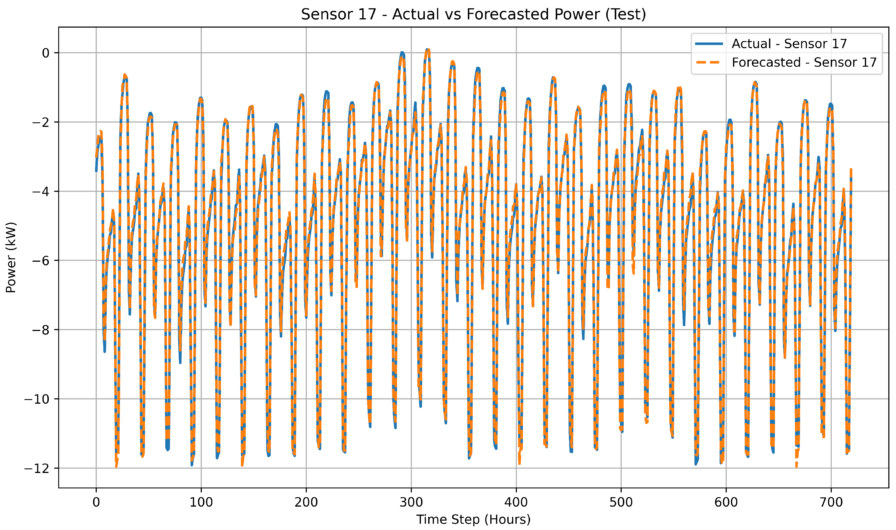
Figure 9 shows the comparison between actual and forecasted measurements for sensor 17 on the unseen test horizon to evaluate the temporal generalization capability of the proposed model. The close alignment between predicted and true values demonstrates the model’s ability to maintain forecasting accuracy for unseen test data.

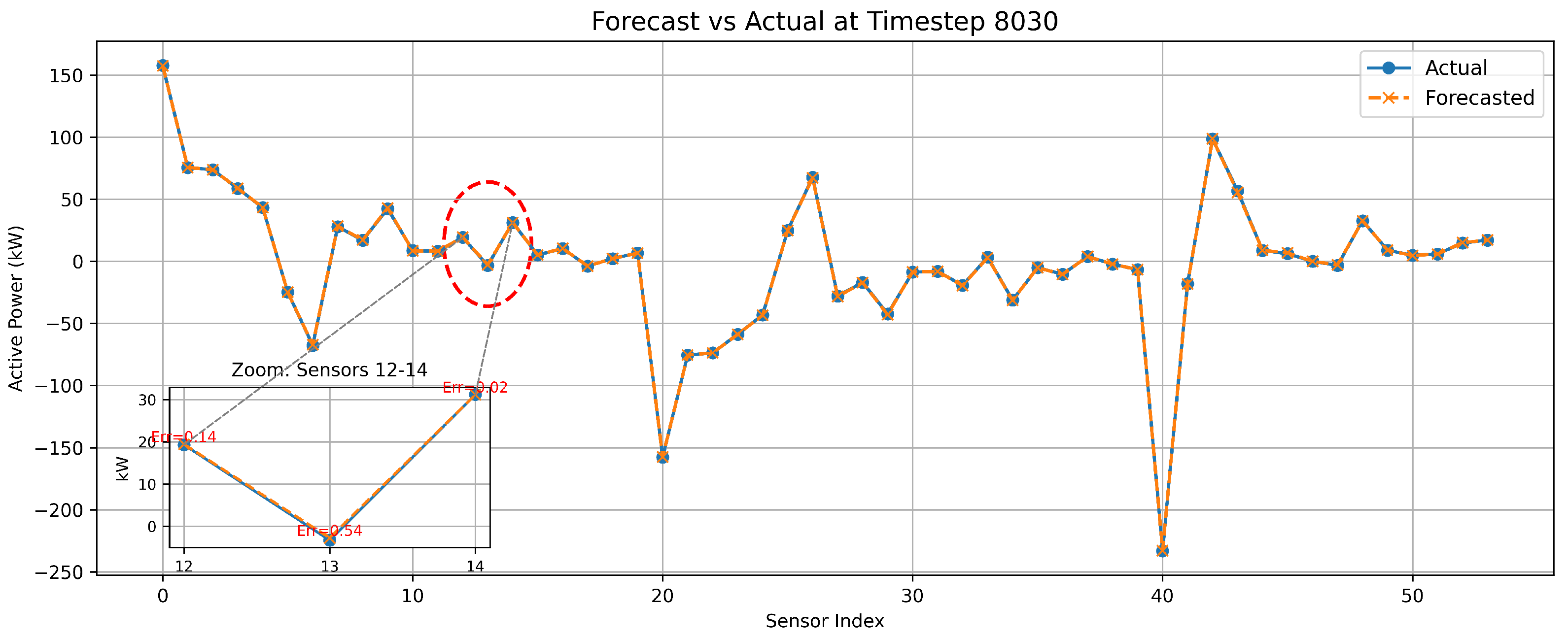
Figure 10 illustrates the comparison between the forecast of the proposed model and actual measurements at 8030 timestep, with a zoomed-in view that highlights three consecutive sensors and their respective absolute errors. The threshold for FDIA detection was determined based on the forecast error, as defined in Equation (30).

Table 2. Performance comparison of FDI detection model using Thresholds.

Model	Threshold	Precision	Recall	F1-Score
Transformer-2LSTM	0.4844	0.993	1	0.986
CNN-BiGRU	0.6957	0.0003	0.0159	0.9756
CNN-BiLSTM	0.4586	0.0003	0.0166	0.975
CNN-BiGRU-Tr	0.4256	0.0003	0.0168	0.9747
CNN-BiLSTM-Tr	0.4444	0.0003	0.0167	0.9748
Proposed Model	0.4191	1	0.997	0.999

presents the performance comparison of various models using this thresholding approach. The optimal threshold for each model was determined to maximize detection performance. For the proposed model, we added a 0.02 margin to the maximum L2 norm observed in benign samples to reduce the risk of false negatives. Since the proposed model achieved the lowest MAE and MSE and the highest R², its forecast was the most accurate, resulting in the lowest optimal threshold among all models. Consequently, the proposed model achieved the best precision, recall, and F1-score for the IEEE 14-bus system. This robustness makes it highly suitable for deployment in critical infrastructure environments for smaller transmission systems.

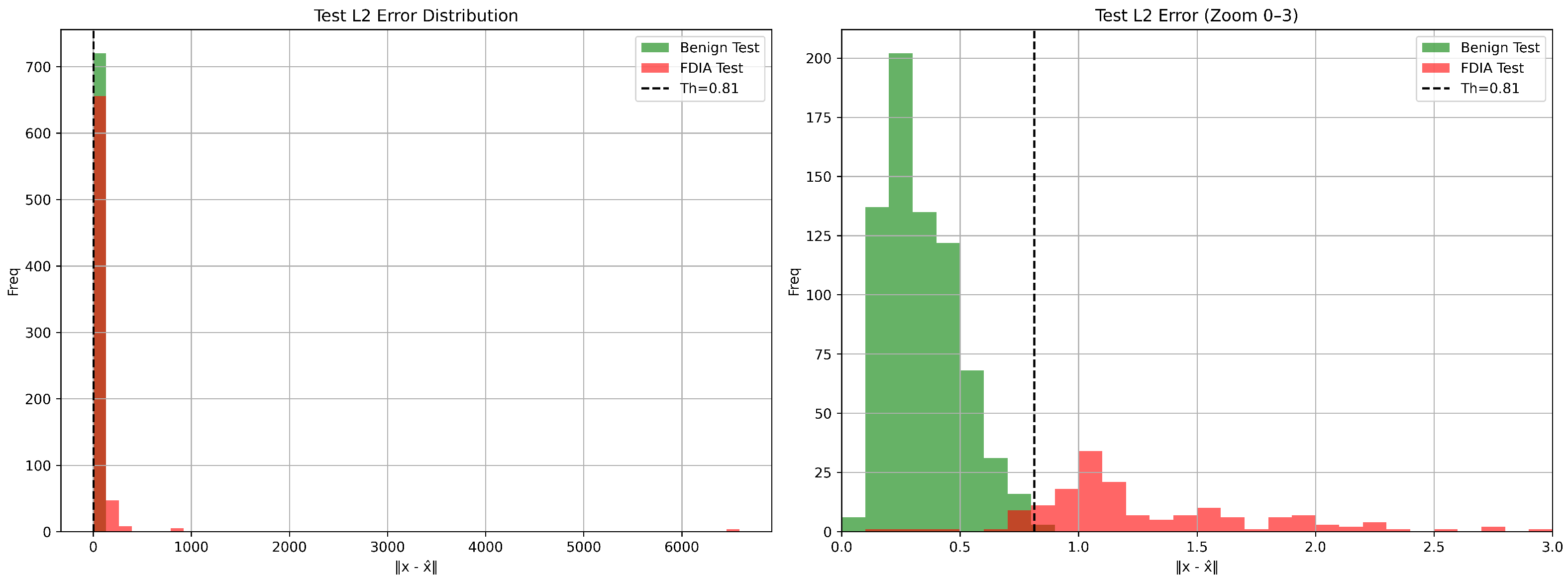
The detection performance of the proposed model is further illustrated in Figure 11, which shows the L2 norm distribution of the normal and attacked test samples along with the selected detection threshold.

Following threshold-based FDIA detection, localization of the compromised sensors was performed using multilabel classification models, namely an MLP and a Random Forest. The input to these models consisted of the error vectors derived from the difference between forecasted and observed measurements, enabling sensor-level identification of tampered signals.

Table 3. Performance comparison for FDIA localization on Unseen Test Data.

Model	Precision	Recall	F1-Score	RACC
MLP	0.9987	0.9985	0.9986	0.9639
RF	0.9966	0.9969	0.9968	0.9486

presents a comparative analysis between the proposed multi-label MLP model and an RF classifier to evaluate their effectiveness in FDIA localization. Although time series classification models were initially considered, their performance was significantly lower in accuracy. Moreover, due to the requirement for real-time inference, the problem was reframed as a multilabel classification task based on forecast error vectors. Consequently, we focus our analysis on the two best-performing models suited for rapid, sensor-level attack localization.

Table 3 shows that both models demonstrate high precision, recall, and F1-score, confirming their effectiveness in accurately identifying FDIA-compromised sensors. However, the MLP slightly outperforms the RF in most of the metrics, particularly in RACC, where MLP achieves 0.9639 compared to RF’s 0.9486. Although the RF maintains high precision, recall, and F1-score, it may still misclassify one or more sensor labels in a single timestep. This results in lower RACC, as it only considers predictions as correct when all labels for an instance are accurate. In contrast, the MLP model performs well in individual sensor metrics and maintains better consistency across all labels per timestep. This makes MLP more robust for system-wide FDIA localization, especially in scenarios requiring reliable performance under real-time constraints.

5.2. Scenario 2: FDIA Detection and Location Module in IEEE 118–Bus System

In the second case, we investigated the performance of the proposed forecasting model for the IEEE 118–bus system to evaluate the scalability and robustness of the proposed framework for large transmission networks. The same two-stage methodology was employed, where the parallel hybrid CNN and Tr-BiLSTM model was first trained to forecast system variables. The performance of the forecasting model for the IEEE 118–bus system is shown in

Table 4. Performance comparison of the Forecasting Module for the IEEE 118–bus system.

Model	MAE	MSE	RMSE	${\mathit{R}}^2$
Transformer-2LSTM	0.009	0.0002	0.0142	0.9406
CNN-BiGRU	0.0116	0.0003	0.0166	0.9394
CNN-BiLSTM	0.0133	0.0003	0.0187	0.9415
CNN-BiGRU-Tr	0.0106	0.0002	0.0154	0.9415
CNN-BiLSTM-Tr	0.0154	0.0005	0.0226	0.9325
Proposed Model	0.0117	0.0003	0.0169	0.9387

.

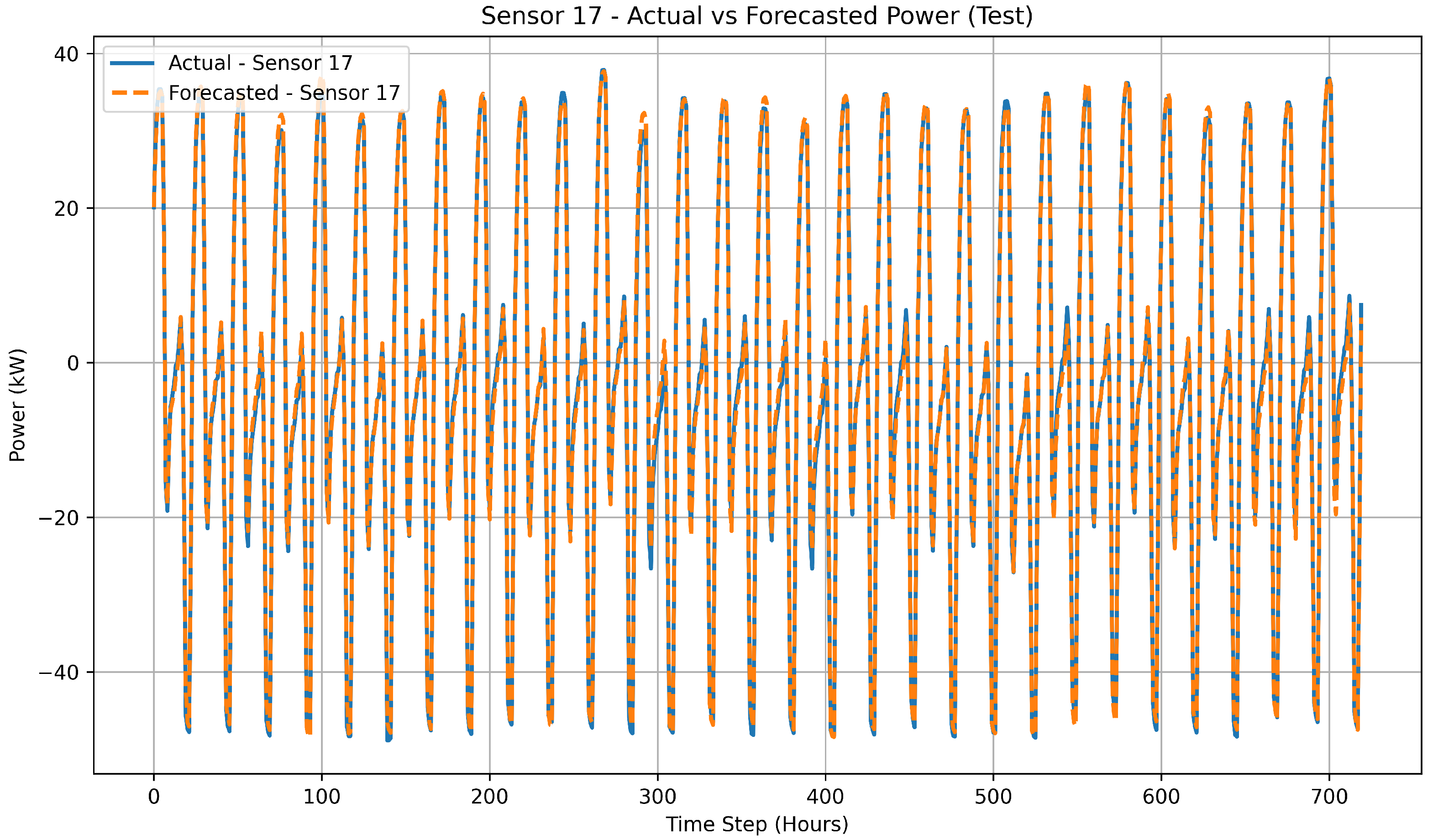
Figure 12 shows the comparison between actual and forecasted measurements for sensor 17 on the unseen test horizon to evaluate the temporal generalization capability of the proposed model.

Figure 13 shows the comparison between the predicted measurement of the proposed model and the actual measurement at 8030 timesteps, with a zoomed-in view that highlights three consecutive sensors and their respective absolute errors.

The FDIA detection using a threshold-based approach was implemented, and the performance of the proposed model was evaluated.

Table 5. Performance of proposed model for the FDI detection model using thresholds in IEEE 118–bus System.

Model	Threshold	Precision	Recall	F1-score
Transformer-2LSTM	0.8526	1	0.972	0.986
CNN-BiGRU	0.8828	0.996	0.971	0.983
CNN-BiLSTM	0.8295	0.989	0.987	0.988
CNN-BiGRU-Tr	1.3309	1	0.833	0.909
CNN-BiLSTM-Tr	1.0225	0.999	0.933	0.965
Proposed Model	0.8133	0.996	0.979	0.988

shows the performance of the FDI detection model using a threshold approach.

The detection performance of the proposed model is further illustrated in Figure 14, which shows the L2 norm distribution of the normal and attacked test samples of the unseen test data along with the selected detection threshold.

Subsequently, multilabel classification was used to locate compromised sensors based on forecast error vectors. As before, both an MLP and a Random Forest model were evaluated for comparative localization performance.

Table 6. Performance comparison for FDIA localization on Unseen Test Data for IEEE 118–bus System.

Model	Precision	Recall	F1-Score	RACC
MLP	0.9965	0.9944	0.9955	0.8430
RF	0.9963	0.9875	0.9918	0.8556

presents a comparative analysis between the proposed multi-label MLP model and the RF classifier to evaluate their effectiveness in FDIA localization.

In comparison to the IEEE 14–bus system, all forecasting models demonstrate scalable performance when applied to the IEEE 118–bus system. However, a consistent decline of approximately 3 to 4 percentage points is observed in $R^2$ for all models. This is likely due to the increased complexity of the system, the larger number of features, and the greater interdependence among variables. Although the Transformer-2LSTM model achieved the best average forecasting accuracy, the proposed method yielded the minimum detection threshold among all models evaluated. This outcome is likely due to the Transformer-2LSTM model producing occasional large deviations in its predictions, unlike the proposed model. Since the L2 norm is sensitive to such deviations, the small outlier can disproportionately increase the overall threshold. In contrast, the proposed model maintains robust and consistent forecasting performance, threshold settings, and FDIA detection in the larger system. For localization, MLP attained higher per-label precision, recall, and F1-score, but RF again outperformed MLP in RACC (0.8566 vs. 0.8430), confirming its robustness in maintaining inter-label consistency for multilabel classification. The drop in RACC is expected since the IEEE 118–bus had 490 features compared to 54 features for the IEEE 14 system, increasing the likelihood of row-level misclassification due to a single erroneous sensor prediction. These results demonstrate that the two-stage forecasting and localization framework remains effective and generalizes well to larger grid configurations when appropriately retrained.

5.3. Scenario 3: FDIA Detection and Localization with Stealthier Attack Vectors

In order to investigate the resilience of the proposed Location Detection Module, we considered a scaling-based stealthy attack strategy. Original attack vectors A are scaled down to fractions such as $3A/4$, $2A/3$, and $A/2$, as explained in Section 4.3. These progressively subtler attacks introduce minimal perturbations to the true measurements, making them harder to detect.

Table 7. Performance comparison of proposed model for FDIA localization using Threshold-based approach.

Model	Threshold	Precision	Recall	F1-Score
IEEE 14–bus	0.4191	1	0.9681	0.9838
IEEE 118–bus	0.8133	0.9954	0.9069	0.9491

summarizes the performance of the proposed approach in different attack strengths using the threshold-based approach for the IEEE 14 and 118 bus systems. The results highlight sustained performance in all metrics for the IEEE 14 and 118 bus systems, confirming its applicability for larger systems.

Table 8. Performance comparison of RF and MLP for FDIA localization across scaled attack levels.

Model	System	Precision	Recall	F1-Score	RACC
MLP	14-Bus	0.9976	0.9967	0.9972	0.9197
MLP	118-Bus	0.9949	0.9945	0.9947	0.8188
RF	14-Bus	0.9913	0.9916	0.9914	0.8326
RF	118-Bus	0.9938	0.9903	0.9921	0.8005

presents the localization performance of the RF and MLP models under different levels of scaled FDIA, highlighting their ability to detect stealthier FDIA attacks. Although the RACC of both RF and MLP dropped similarly to the threshold-based approach, MLP was consistent in its performance compared to the RF and threshold-based approach.

The results in Table 7 and Table 8 show the performance degradation as the FDIA becomes more stealthy, affecting both the threshold-based detection and the RF and MLP-based localization models. This drop shows that fixed thresholds struggle against small perturbations. Similarly, the RF and MLP classifiers maintain relatively stable precision, recall, and F1-scores across scaled attack levels. Although RF outperforms MLP in RACC under unscaled attack conditions in 118-bus systems, its performance degrades under scaled attacks. Since RF is an ensemble of decision trees, it prioritizes features with higher variance and fails to capture the subtle deviations introduced by low-magnitude attacks. In contrast, MLPs, with their ability to capture complex nonlinear dependencies and continuous feature relationships, demonstrate more stable inter-label consistency across scaling levels. These results collectively suggest that while both models handle individual sensor classification reliably, preserving full multilabel accuracy becomes increasingly difficult as grid complexity and attack stealthiness increase.

5.4. Scenario 4: FDIA Detection and Localization During DOS Attacks

In order to evaluate the robustness of the proposed detection and localization framework under realistic cyberattack conditions, we considered DoS and FDIA attacks jointly. During a DoS attack, the sensor nodes are out of operation and do not provide any measurements to the central monitoring system. If attackers perform stealthy FDIA during DoS simultaneously, the threshold-based detector or learning-based models will have fewer reference points to validate the authenticity of the incoming data. This will allow false data to bypass the FDIA detection system.

In this evaluation scenario, different combinations of buses are selected to simulate DoS attacks, including all single-bus cases, all two-bus combinations, and all three-bus combinations. These attacks render the measurement data from all sensors in the selected buses unavailable. The mapping between each bus and its corresponding sensor is provided in Figure 7. At the same time, an FDIA is performed on another random subset of the remaining active sensors. Within the proposed framework, missing data from sensors of all DoS-affected buses are replaced with their corresponding forecasted values before being passed to the multiclass classifier, such as an RF or MLP. This strategy ensures that the model can continue processing inputs despite partial data loss.

Table 9. Performance comparison of RF and MLP for FDIA localization during DoS attack.

Bus Combination	Model	Precision	Recall	F1-Score	RACC
1	MLP	0.9985	0.9980	0.9983	0.9670
1	RF	0.9944	0.9956	0.9950	0.9443
2	MLP	0.9985	0.9985	0.9985	0.9736
2	RF	0.9944	0.9966	0.9955	0.9533
3	MLP	0.9985	0.9988	0.9987	0.9796
3	RF	0.9940	0.9967	0.9954	0.9567

presents the average localization performance of the proposed framework in different numbers of DoS-affected buses. For each configuration, we report the average values of Precision, Recall, F1-score, and RACC to evaluate the robustness of the framework under varying levels of sensor unavailability.

Both RF and MLP classifiers demonstrate high precision, recall, and F1-scores in identifying individual FDIA-compromised sensors, which confirms their effectiveness in feature-level detection for the IEEE 14–bus in a DoS and FDIA attack scenario. In addition, both models maintain high RACC under the partial observability condition. MLP achieves a higher RACC compared to RF for every scenario. This robustness is likely due to its dense architecture, which allows for effective generalization of the FDIA attack patterns under partial observability. This upward trend for both models can be attributed to multi-bus attacks introducing more distinguishable and redundant forecast errors, improving the model’s ability to infer the full attack vector. Larger-scale attacks lead to denser label vectors and more prominent deviations from normal behavior, making the attack easier to detect despite DoS-masked input. Although both models demonstrate strong generalization to FDIA and DoS conditions without retraining, the MLP model provides the most consistent and robust performance across all levels of attack severity.

6. Conclusions

This paper presents a robust and scalable machine learning framework for the real-time detection and localization of FDIA in SGs. The proposed multistage architecture combines a parallel CNN and sequential Tr-BiLSTM-based forecasting model with a multilabel classification module that uses an MLP or RF to locate compromised sensors using forecast error vectors. The framework is evaluated across multiple benchmark power systems under various adversarial conditions, such as FDIAs with varying attack magnitudes and combined FDIA-DoS scenarios.

Comprehensive evaluations on IEEE 14-bus and 118-bus test systems demonstrate that the proposed framework outperforms the existing ML architecture in the forecasting and FDIA detection performance. The L2-norm thresholding method, based on the proposed forecasting method, is effective for detecting unscaled attack vectors, but its performance deteriorates slightly for the IEEE 118–bus system and scaled attack vectors. Both the RF and MLP classifiers achieve high RACC in sensor-level localization. The RF classifier is more effective for unscaled attack vectors and in large transmission networks, whereas the MLP shows greater resilience against subtler FDIA attacks and DoS-induced sensor outages for all transmission networks.

Unlike traditional single-stage detection systems or a multilabel classification approach, the proposed multi-stage framework offers greater flexibility and reliability in detecting and localizing FDIA scenarios, even in the presence of missing sensor data. However, the present study is limited to benchmark test systems and simulated attack environments and does not consider dynamic grid topologies such as reconfigurations or contingency-driven structural changes. Future work will explore the performance of the proposed model in dynamic grid topologies caused by contingency events, maintenance operations, and system reconfigurations to enhance its applicability to real-world transmission systems.