Highlights
What are the main findings?
- A novel integrated approach is presented for long-term hourly traffic predictions, based on LSTM, that shows good performance and accuracy, with high fidelity in periodicity and variability across diverse traffic profiles in California.
- By leveraging Fourier Transform, the sliding window approach, and K-means, the presented approach expands the traditional LSTM, capturing traffic hourly pattern and flow intensity over a year’s time frame.
What is the implication of the main finding?
- Accurate long-term hourly prediction is critical for a sustainable and resilient transportation system and therefore deserves more attention and research efforts.
- The present study makes good strides toward the use of sophisticated ML models for long-term traffic forecasts, an area still widely unexplored.
Abstract
Traffic conditions are a key factor in our society, contributing to quality of life and the economy, as well as access to professional, educational, and health resources. This emphasizes the need for a reliable road network to facilitate traffic fluidity across the nation and improve mobility. Reaching these characteristics demands good traffic volume prediction methods, not only in the short term but also in the long term, which helps design transportation strategies and road planning. However, most of the research has focused on short-term prediction, applied mostly to short-trip distances, while effective long-term forecasting, which has become a challenging issue in recent years, is lacking. The team proposes a traffic prediction method that leverages K-means clustering, long short-term memory (LSTM) neural network, and Fourier transform (FT) for long-term traffic prediction. The proposed method was evaluated on a real-world dataset from the U.S. Travel Monitoring Analysis System (TMAS) database, which enhances practical relevance and potential impact on transportation planning and management. The forecasting performance is evaluated with real-world traffic flow data in the state of California, in the western USA. Results show good forecasting accuracy on traffic trends and counts over a one-year period, capturing periodicity and variation.
1. Introduction
Accurate traffic prediction is essential in shaping smart transportation systems and future mobility systems. For example, good traffic volume prediction can help with infrastructure utilization efficiency, urban development planning, traffic management strategies, and even environmental impact assessment. Understanding when and where traffic volumes are highest/lowest allows for more efficient use of existing infrastructure and informed development decisions, given insights into traffic volume dynamics. Traffic volume dynamics during the day, for instance, may help with the implementation of signal timings adjustments or traffic signal coordination optimization. The environmental impact on the transportation network through carbon footprint analysis [1] can also be estimated.
This can hardly be achieved without rich and large-scale data, capturing the time and spatial variability of traffic trends. As more interest is shown toward mobility, the size of data and data sources are growing rapidly. The high volume of data captured, managed, and analyzed is certainly positive for transportation analysis. Transportation data are now complex and large-scale, spatially distributed, and dynamic/transient [2]. These characteristics widen the opportunities for mobility analysis, helping to investigate issues yet to be addressed, and leading to the development of advanced methods/models/tools. With the availability of rich data, analytics, and data fusion/merging/handling tools, there is a tremendous opportunity for in-depth analyses that can lead to advancements in transportation infrastructure and reduce the environmental impacts of vehicular traffic. These analyses provide a competitive and innovative advantage, first because large volumes of data inputted into fairly simple models often offer better and more accurate insights than sophisticated learning algorithms with scarce data [3], and second, because large volumes of data fuel the motivation for the sophistication of the models themselves, by virtue of which new insights can be reached [4]. Data quality, for instance, although a concern, encourages state-of-the-art approaches to take full advantage of available data and perform meaningful analysis [5]. Large-scale and complex data are thus invaluable in understanding our transportation systems, helping to support next-generation traffic management systems and face related issues.
Several methods have been used for traffic prediction, including Naïve models using clustering or historical averages [6], Hidden Markov [7,8], autoregressive integrated moving average (ARIMA) [9,10], and Kalman filtering techniques [9,11]. Other methods like k-NN (nearest neighbor) [12,13] and Neural Networks [14,15] have also been employed. The k-nearest neighbors (KNN) algorithm, a non-parametric, supervised learning classifier, is a method of pattern recognition using past data for prediction [16]. As opposed to other methods, Neural Network models are flexible as they can learn from the data, and are known to better capture complex spatial-temporal characteristics and the nonlinear trends of traffic flow [17]. Deep learning (DL) Neural Network (NN) approaches have been proven to extract temporal features from time series data, including Convolutional Neural Networks [18,19] and Recurrent Neural Networks [20,21]. Approaches using DL algorithms have been focused on short-term traffic flow prediction [9,22]. Short-term traffic time intervals used are usually in the range of 5 min to half an hour [23].
Intelligent transportation systems (ITS), which have attracted wide attention from researchers [24], require effective ways to minimize congestion, which has been labeled as one of the main problems in urban areas [25,26]. Short-term traffic prediction has been proven to be an effective way to address congestion issues [27], helping riders avoid high-intensity traffic volume and save time and money, as well as reduce gas emissions. Although one of the core needs in the development of ITS, short-term traffic prediction is only one piece of the puzzle. Long-term forecasts help with more strategic decision-making, like infrastructure planning and economic planning. Such forecasts enable preemptive strategies for road control, including congestion mitigation, as well as maintenance planning, especially in urban areas [28]. The movements of people, via buses, bike-sharing programs, EVs, shared mobility, or connected/automated vehicles, experiencing changes in pattern will drive demand in route preference, charging infrastructure, and energy demand, which will all affect long-term volume. Additionally, these predictions also help businesses anticipate demand patterns and facilitate decisions for facility locations and distribution networks.
Although critical, long-term traffic prediction research is pretty sparse, He, Chow [29] presents a spatiotemporal Convolutional Neural Network (STCNN) based on convolutional long short-term (LSTM) memory units and leveraging the spatiotemporal correlations from historical traffic data predictions. Historical data spans four consecutive weeks, and the model predicts traffic seven days in advance. Wang, Su [30] proposes a DL architecture which consisting of two parts: LSTM encoder–decoder structure at the bottom and the calibration layer at the top. The authors propose a hard attention mechanism based on learning similar patterns, aiming to enhance neuronal memory and reduce error propagation accumulation. The predictions were made on a single day, with different time steps, namely 80, 100, 150, and 288. Xu, Di [31] models traffic as a Gaussian process and uses an attentive graph neural process (AGNP) to learn and predict short-term traffic. By taking a stochastic approach, the model outputs are distributions (and not deterministic static values), giving more insight into the range of possible values for the traffic. Park, Kim [32] approach looks to determine the potential impacts of meteorological information on long-term traffic volume prediction. A Graph Convolutional Network (GCN) was built to predict hourly traffic volume over a week-long time frame. In Lin, Dai [33], a new approach, Short-Term and Long-Term Integrated Transformer (SLIT), was introduced to effectively handle both short-term and long-term traffic patterns predictions. Tests were run over a one-to-seven-day period. In their paper, Berlotti, Di Grande [34] proposes a two-level Machine Learning (ML) methodology involving the use of clustering and forecasting models. Their model makes traffic predictions over two weeks. Guo, Zhang [35] utilize the same ML architecture used in large language models (LLMs)—transformers—to predict traffic in the short term. They incorporate meteorological data, previous traffic data, and holiday information for the greater Los Angeles area to train the Llama2 LLM [36] to predict the next 12 h of traffic. They find that the transformer approach performed comparatively better in the short-term prediction but struggled in the longer time horizons.
The accelerating changes in urban mobility and infrastructure demands warrant more efforts into long-term traffic prediction research. Models for long-term traffic models have to capture the periodicity and variation in real-world data, which is crucial for forecasting [37]. Periodicity represents regular changes in traffic flow on weekdays and weekends, for instance. Fluctuation reflects traffic flow changes at a specific time of the day, peak and off-peak hours, which can be due to a variety of factors like unexpected events (accidents, traffic stops, etc.), weather changes, or social activities. Fluctuations can impact traffic periodicity, affecting the accuracy of long-term traffic flow forecasts [38]. With most research efforts spent on short-term traffic prediction, long-term forecasting presents considerable challenges that have still not been addressed. The lack of significant research in long-term traffic prediction, capturing complex dynamics of long sequences as well as dependencies, is illustrative of the inadequacy of current research and thus highlights the urgency and value of the study presented here. This study is therefore timely and needed, promoting sustainable mobility and accessibility for all community members.
Different from the research discussed before, this present work leverages a large-scale traffic dataset spanning all US states and predicts over a significantly longer period, that is, one year. In this paper, the team presents a method for long-term traffic prediction, leveraging LSTM, K-means clustering algorithms, and the Fourier transform (FT). FT is a time-series analysis method to model periodicity [39]. By integrating FT, traffic data can be decomposed into its constituent frequencies, and periodical behaviors hidden in the series can be revealed [40]. It is particularly useful in analyzing periodicity and extracting frequency information, making it a powerful tool for traffic volume prediction. As traffic often exhibit periodic patterns, such as daily, weekly, or seasonal cycles, FT helps identify these patterns by transforming the time–domain traffic data into the frequency domain, revealing the dominant frequencies that correspond to these cycles [39]. By incorporating frequency–domain information, these periodic trends can be more accurately captured, and forecast accuracy can be improved. LSTM has been used in traffic volume prediction research [10] and has proven efficient in time series prediction. K-means is used to cluster traffic volume data to unearth different traffic flow patterns [41], facilitating the handling of large-scale data. This integration, coupled with the sliding window approach and the previous year’s traffic value as an input feature, provides high accuracy over a year. This constitutes a considerable breakthrough in long-term traffic prediction, which remains widely unexplored. Our contributions can be summarized as follows:
- The team proposes a two-level ML methodology for long-term traffic prediction that leverages k-means clustering, long short-term memory (LSTM) neural networks, and FT. The technique is scalable and can be applied to large datasets, making it suitable for analyzing traffic volumes across extensive road networks or regions.
- The team evaluates the proposed method on a real-world large-scale traffic dataset collected from the U.S. Travel Monitoring Analysis System (TMAS) database, enhancing its practical relevance and potential impact on transportation planning and management. The availability of such data, rich and comprehensive, motivates the development of the modeling approach presented here.
The long-term forecasting approach and model presented here offer a valuable tool for mobility goals, with long-term urban development and driving behavior changes. This research thus helps support scalable mobility systems and aims to ensure future demand is met efficiently. The remainder of this paper is organized as follows: the next section will describe the proposed method used for this study, as well as the methods used to analyze the traffic data. Section 3 describes the experiments, while Section 4 presents the results and discusses their implications. Section 5 concludes the research.
2. Methods and Data
2.1. Data Collection
The data used for this analysis are traffic volume data collected from open-source databases published by the Travel Monitoring Analysis System (TMAS) [42]. The TMAS program aims to provide a comprehensive view of the entire road network in the United States. Data is collected by over 7700 monitoring sites located on various types of roads, including highways, major roads, and local streets, depending on the monitoring infrastructure in place. The data collected provides valuable insights to analyze traffic patterns, congestion, and overall road usage. TMASs are deployed in both urban and rural areas to capture a comprehensive picture of urban and rural mobility. Data types collected include traffic volume (year, month, day, and hour), location (state, latitude, and longitude), vehicle speed, occupancy, and sometimes more detailed information such as vehicle classifications.
Another data program, the Highway Performance Monitoring System (HPMS) [43], is also publicly accessible. The HPMS program includes inventory information for all of the Nation’s public roads, that is, roads open to public travel, including interstates, freeways and expressways, principal and minor arterials, minor and major collectors, as well as local roads [44]. Data types collected include traffic volume (yearly average), location (state, latitude, and longitude), route details (identification, segment start and end, segment length), and similarly to the TMAS, vehicle speed, occupancy, and sometimes more detailed information such as vehicle classifications.
Both programs help make informed decisions about infrastructure development, traffic management strategies, and other interventions to improve overall transportation efficiency. The differences between those systems lie at two levels: spatial and temporal granularity. Spatially, HPMS offers finer granularity, focusing on the analysis of traffic patterns on specific road segments, rather than areas. Segments are stretches of road characterized by start and end points, as well as length. Fine-grained origin-destination data, with information on the starting and ending points of trips, helps in understanding travel patterns, commuter routes, and the flow of traffic between different routes. Temporally, TMAS offers finer granularity, that is, hourly vehicle counts (which can help infer seasonal variations), rather than only the yearly average count. Higher temporal granularity allows for the identification of peak hours, rush periods, and variations in traffic flow throughout the day. Figure 1 displays dataset information for California. As the intent is hourly traffic prediction, TMAS data is used in this study.
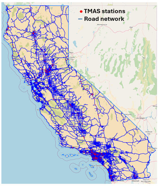
Figure 1.
California road system and TMAS Stations.
2.2. Methodology
In this research, a long-term traffic prediction method is proposed as detailed in Figure 2. The proposed methodology consists of three steps. In the first step, TMAS traffic counting stations were grouped into several groups based on their traffic volume. In the second step, historical traffic volume data for each group was used to train deep learning models for long-term prediction of traffic. In the last step, the models were trained to predict hourly traffic volumes for each group.
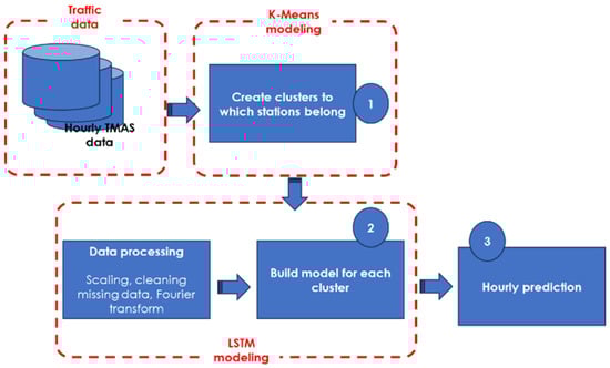
Figure 2.
Methodology for traffic volume prediction using ML models and data integration.
Step 1—TMAS stations are located along highways and routes in the U.S. and record a substantial amount of traffic data. K-means, an unsupervised algorithm that handles scalability for large datasets [45] helps group together stations with similar traffic volume patterns. This step simplifies complexity and reduces the size of the data, with the intention of improving the performance of subsequent algorithms. What is needed in this step is a way to preprocess all the traffic stations’ data, classifying them together based on some similarities, to improve the accuracy and explainability of the prediction. Segmenting stations into meaningful groups can help uncover underlying patterns/similarities, enabling the analysis to be more specific to each group. Highways, urban arterials, and other roads often have distinct patterns, which are reflected by the recordings from TMASs. K-means is chosen for this purpose due to its simplicity and interpretability. K-means is a centroid-based clustering algorithm, categorizing N observations, in our case, monitoring stations, into K clusters [3]. Clusters are formed given their annual average traffic volume, following Equation (1):
where VOLs is the average daily traffic volume calculated for a given station s, Voly is the sum of vehicle counts over year y, and nb_day_y is the number of days over which the counts were recorded in that very year y. Traffic data considered for clustering range from 2011 to 2021. The stations are grouped by cluster based on squared distance from the centroid of that cluster [46]. A centroid is a data point representing the center of the cluster. The algorithm iterates until each data point is closer to the centroid of its cluster than to the centroids of other clusters, minimizing intra-cluster distance at every step. The mathematical representation follows Equation (2) [47]:
where E is the squared error function, xij is a station i assigned to cluster j, and xj is the centroid of cluster j. The objective is to minimize E [48]. K-means requires a predefined value of K, the number of clusters. In our case, 3 clusters were selected, after running the algorithm with different numbers of cluster sizes, including 2, 3, 4, and 5. Figure 3 shows the 2-dimensional visualization using PCA (principal component analysis). Points displayed illustrate stations with different colors, representing the clusters they belong to. The figure shows a good separation of stations, with minimum overlap, indicating an appropriate number of clusters. The different cluster profiles therefore show different traffic patterns: low traffic category (cluster 1), mid traffic category (cluster 2), and high-traffic category (cluster 3).

Figure 3.
Stations visualization per cluster, projected to 2-dimensional points using PCA.
Step 2—LSTM models are created for each of the clusters found in the previous step. Three models are therefore built, using a time series, which will be used as training data. It is assumed that each cluster is represented by a single model, with stations in the same cluster all having the same model. The clustering step intends to categorize stations with similar patterns together to build a unique model, capturing the general traffic trend. Ideally, a model would be built for each station, which is not practical, given the large number of stations and data. Time series, in this study, are a sequence of traffic volume recorded every hour, in a day, a month, and a year. However, some stations have gaps for certain periods of a year. Therefore, the data is processed to ensure that only continuous stretches of data are used as training data for the model. Figure 4 shows an excerpt of the time series.
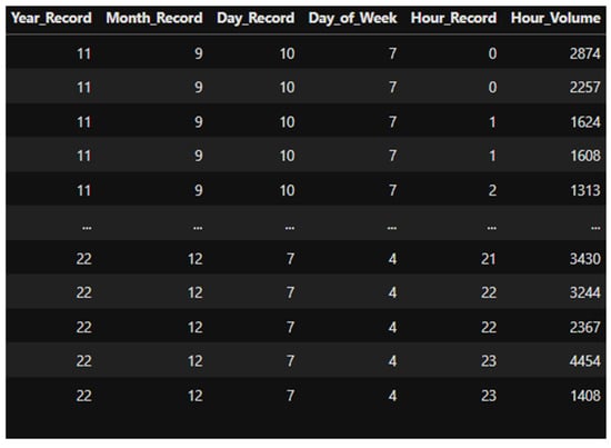
Figure 4.
Excerpt of traffic volume time series.
LSTM is a special type of Recurrent Neural Network (RNN) model, capable of remembering information for a long period of time, and is suitable for time series prediction [45]. RNNs are commonly difficult to train, given the gradient vanishing issue, making it arduous to learn long-term patterns [49]. In its hidden layers, LSTM possesses a memory block that includes layers that store and regulate the information flow. LSTM is capable of learning long-term dependencies due to the structure of its units, which incorporates three gates that regulate the long-term memory and learning process [50]. These gates consist of a “forget gate”, determining the information to discard, an “input gate”, determining the new information to be saved, and an “output gate”, determining what information to output to the next level [51].
The seasonality/variability of traffic volume across the state of California can constitute an obstacle to the LSTM model. This will thus require good model architecture and accurate hyperparameter determination. To train the LSTM models, a sliding window approach was used, considering a sequence of input data to predict the next value in the sequence. The sliding window technique segments the time series data into fixed-length windows, with each window containing a sequence of input features and the corresponding target output. During training, the model receives an input sequence through the LSTM layers, which capture temporal dependencies and patterns in the data, and then predicts the next value in the sequence based on the learned information. By using this approach, the model learns to recognize patterns and make predictions beyond the window size. In our case, a window of 30 h of traffic volume is used to predict the 31st hour. This is to capture trends of each previous day and a few hours (6 h) before/after to ensure the model can recognize the start/end of a day. In addition to this sequence of input data, the previous year’s traffic value for the 31st hour is also used as an input,. The previous year’s traffic value is considered as an input/feature to handle different peaks and make the model training more stable. This ensures that the model interprets the input data correctly. Data processing follows standard machine learning practices such as scaling (min-max scaling) to ensure the input features are of a similar magnitude. Furthermore, the scaled 30 h window is Fourier transformed to better capture periodicity and extract latent information from the inputs [52]. The Fourier-transformed features are split into separate real and imaginary time series and fed into the LSTM alongside previous years’ traffic values. Using that decomposition technique helps separate seasonality and trends from the traffic volume data before feeding it into the LSTM model. This can help the model focus on the underlying patterns without being overwhelmed by non-stationary components. Figure 5 illustrates the training approach.
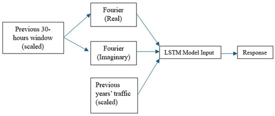
Figure 5.
Training features in a time-series format.
Step 3—In this step, hourly predictions are made over the next year, that is, 2022. Traffic volume for all the days of that year is forecasted.
3. Experimental Setup
3.1. Dataset Description
TMAS data collected from the U.S. state of California was used for model training and evaluation. Training data for each cluster ranges from the year 2020 to 2021 (the first 70% of this period), and testing data covers the year 2021 (the remaining 30%). After disregarding stations that had a limited history in available traffic data, the number of stations for clusters 1, 2, and 3 were 61, 19, and 8, respectively. This resulted in training size input of 756,908, 217,769, and 93,421 hourly data points, respectively.
3.2. Hyperparameter Optimization
Hyperparameters are configurable variables that control the model’s architecture, learning process, and its complexity. These variables are set before the training begins. Common hyperparameter tuning methods like grid search or random search tend to be time-consuming. Although showing promise and efficiency, they can be computationally expensive, especially for complex models such as deep learning neural networks [53]. Optuna, introduced by [54], is a hyperparameter optimization framework, enabling the dynamic parameter search space, efficient implementation of both searching and pruning strategies, and a versatile architecture that can be deployed for various purposes [54]. Optuna’s pruning feature helps prematurely terminate runs that are not optimal, which is possible thanks to an asynchronous successive halving algorithm [55]. Compared to other advanced hyperparameter optimization techniques like Scikit-opt and HyperOpt, Optuna, using the Tree-structured Parzen estimator (TPE) search algorithm and Expected Improvement (EI) acquisition function, has been shown to perform better, showing the highest efficiency for both CNN and LSTM models [56]. In our study, Optuna was thus used to determine the optimal hyperparameters for our LSTM model. The model architecture can be found in Table 1.

Table 1.
LSTM hyperparameters.
3.3. Experiments
The proposed approach was evaluated in two ways: (test 1) prediction accuracy performed based on real traffic volume, and (test 2) prediction accuracy performed based on previous predictions. In the 1st test, the input sequences are the real data from the year 2022. In the 2nd test, input sequences are the first 30 h of 2022 to initialize the prediction flow, and further predictions are made using the sliding window for further predictions. Given the sliding window approach used for prediction, it is critical to estimate the accuracy of predictions from the LSTM models, which are based on previous predictions. Is there any significant drop in performance and accumulation of errors when the LSTM model predicts traffic volume values in the long-term future?
4. Results and Discussion
The prediction evaluations are shown in Figure 6, Figure 7 and Figure 8 for test 1, Figure 9, Figure 10 and Figure 11 for test 2, applied to values for randomly selected 300 h in 2022. Both sets of values are compared to the actual traffic volumes for the same 300 h period in 2022. The predictions are from a station, also randomly selected within a cluster. Results show (1) hourly predictions on the line charts, and (2) error distribution on a histogram chart. The error distribution graph displays prediction errors, calculated by dividing the difference between the estimated value and the original value by the original value. Figure 6, Figure 7 and Figure 8 display the model’s performance on predicting traffic volume for a random station in the state of California for clusters 1, 2, and 3, respectively. As can be seen, the predictions look very accurate, with faithful trend-following. Predictions for cluster 1 look more accurate, compared to the ones for clusters 2 and 3. More deviations were observed as traffic volume increased and patterns grew more complex. Predictions tend to overestimate and underestimate, although they adjust in a timely manner. For each cluster, the errors are symmetrically distributed between −20% and 20%, which indicates an equal likelihood of overestimating/underestimating peak/off-peak hours. The low variability indicates that the model performs consistently across hours of the day and different levels of traffic volume. The error distribution displays a bell-shaped curve, suggesting that most errors are small and that large errors are relatively rare, which is illustrated by the bulk of the errors close to 0. Overall, the predicted values are closer to the true values of the ground. The median and the mean absolute error for predictions for each of the clusters are presented in Table 2. As the different clusters have different scales of traffic, the errors are also presented as percentages in parentheses to compare across clusters. The presence of outliers (especially when actual traffic is close to 0) skews the mean and the root mean squared errors to be higher than the median errors for all clusters (especially for percentages).
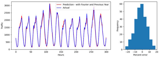
Figure 6.
Test 1 evaluation over a 300 h interval and error distribution for Cluster 1.
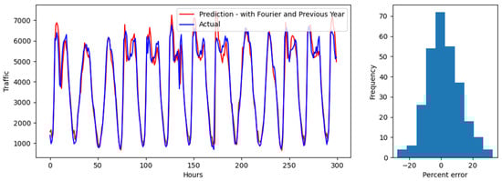
Figure 7.
Test 1 evaluation over a 300 h interval and error distribution for Cluster 2.
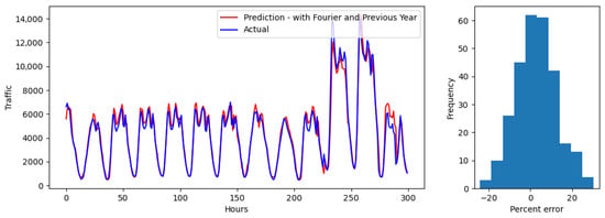
Figure 8.
Test 1 evaluation over a 300 h interval and error distribution for Cluster 3.
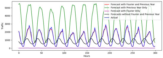
Figure 9.
Test 2 evaluation over a 300 h interval, 200 days after initialization, for a random station in Cluster 1.
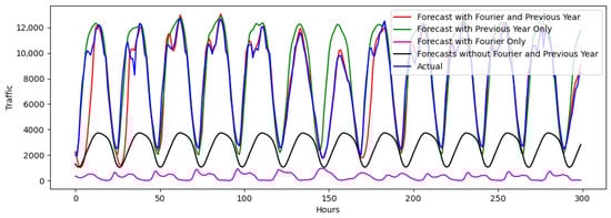
Figure 10.
Test 2 evaluation over a 300 h interval, 200 days after initialization, for a random station in Cluster 2.
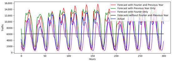
Figure 11.
Test 2 evaluation over a 300 h interval, 200 days after initialization, for a random station in Cluster 3.
Table 2.
Median absolute error, mean absolute error, and root mean squared error for predictions for all clusters.
Figure 9, Figure 10 and Figure 11 show the model performance for test 2, and their corresponding errors are shown in Table 3. In this test, each prediction becomes one of the inputs in the model for the next prediction, as described in the “sliding window” approach. An ablation study was conducted to demonstrate the effects of various components used in the model presented and compare the prediction performance. Results are shown with various permutations of the inclusion/exclusion of FT and the previous year’s traffic as an input. The model that includes both FT and the previous year’s traffic data significantly outperforms the other models, considering periodicity and scale, which are confirmed by the error values, quantifying the magnitude of difference between the predicted and actual values. Models without FT struggled to maintain appropriate periodicity (Figure 9), while those without the previous year’s traffic data struggled to maintain the correct traffic value scale (see Figure 9 and Figure 10). Furthermore, as illustrated in Figure 10 and Figure 11, LSTM alone struggles with past information retention from long sequences, emphasizing the need for more sophisticated strategies [57]. The model is also shown to occasionally “collapse” into a flat line. Upon reviewing the forecasts, it was found that this flatlining occurred because the model incrementally predicted lower traffic peaks with decreasing deviations over the 30 h input period, ultimately resulting in a constant line. For clusters 1 and 2, the best model had a median absolute error lower than 5%. However, for cluster 3, the error was at 16.6%. For each of these clusters, the model predicts well, following the traffic trends. Periodicity is fairly maintained, although, as expected, prediction accuracy dropped. Similarly to the results in test 1, predictions for clusters 1 are more accurate than those in clusters 2 and 3, which exhibit a more complex traffic pattern. The model for cluster 3 tends to overestimate, which can be caused by a variety of things, including scaling issues, vanishing/exploding gradients, or hyperparameter tuning. While LSTMs are designed to mitigate these issues, they can still occur, especially in very deep networks or long sequences, as analyzed in this paper. Another reason could be the nature of the traffic for cluster 3, which has a sharper difference between the bimodal peaks of traffic.
Table 3.
Median absolute error, mean absolute error, and root mean squared error for all clusters and models over the 300 h period.
While the deviation from actual traffic is higher in test 2 than in test 1, which is expected, periodicity, variation, and traffic intensity scale are captured. Forecasted traffic values appear to match the same periodicity of real-life traffic, with no apparent lagging, even 1 year into the future. It is evident that when predictions are made using prior predictions as input (compared to predicting using real-world traffic values for each hour), the errors are higher and magnified. However, they still display a high level of fidelity multiple days into the future (13 days, about 2 weeks), especially capturing weekday/weekend fidelity. In all the results presented, it can be observed that the general shape of traffic is conserved. Common methods, including ARIMA, SVM, SAE, or RBF network, usually employed for performance comparison, are not considered, since they have been proven to perform poorly for traffic flow forecast when compared to LSTM-based methods. See [21,58,59].
Insights from results presented in this paper are not too different from the few long-term efforts undertaken in the literature, although with predictions over a shorter timeframe. Wang, Su [30]’s results show good accuracy and stability in long-term sequence prediction. Their model shows dependence on time step, with increased stability in long-term prediction. The algorithm tends not to be in phase with real data, especially for fewer time steps, and generally tends to undershoot for a location compared to the others. Similarly to our results, the accuracy level varies by location. Berlotti, Di Grande [34], which presents a similar approach to ours, also shows differences in accuracy, depending on location. The results vary in precision, based on the clusters considered. Although these papers make predictions on significantly shorter periods, the impact of differences in traffic patterns by location affects the model’s predictive power. This is what our results show. In this paper, errors tend to be more dependent on locations, or traffic volume profiles, rather than the length of the prediction or time steps, unlike in [30].
The biggest problem with long-term traffic flow forecasting is that errors accumulate. The very nature of a lengthy horizon over which the prediction is made is what constitutes the biggest hurdle. Traffic volumes naturally fluctuate over time due to daily, weekly, and seasonal cycles, with peak hours, weekends, and holidays causing sharp variations. Additionally, geographical differences—such as urban versus rural traffic, road and network configurations further complicate prediction models. These variations make it difficult to develop a model that performs equally well across all locations and time periods, as shown in our model and models in the literature. Another challenge coming with the temporal and spatial variability of data is its size. As traffic networks grow in complexity and scale (e.g., national or regional road networks), predictive modeling challenges grow. Although this work presents only state-level traffic volume analysis, the amount of data was very large. Engaging on a national level would undoubtedly be more challenging. Ideally, given geographical differences in traffic trends and patterns, our approach would apply to each state, that is, building at least 100 LSTM models, assuming 50 states and two clusters each. Another option would be clustering at the national level, which will expectedly require a high number of prediction models, with increased computational complexity. Algorithms like K-Means with a complexity of O(n * k * t), where ‘n’ is the number of data points, ‘k’ is the number of clusters, and ‘t’ is the number of iterations [60] would cause the computational load to become prohibitive as ‘n’ increases. The scalability of our method, even though possible, could be very time-consuming and may very well affect the accuracy of the results. Also, as datasets grow, it becomes harder to evaluate the quality of clusters. Validation metrics like silhouette scores can become computationally expensive. Clusters can also be imbalanced (some very large, some very small), making it easier to skip small clusters, which may be meaningful. Large clusters can dominate the process and distort the results.
There is still room for improvement in this study. The study applies K-Means Clustering to group stations that show similar characteristics, with only traffic volume as input. Types of roads, days of the week (weekday vs. weekend), or seasons (winter, summer, etc.) can be considered to capture spatiotemporal heterogeneity among sites. In addition, the occurrence of public events and holidays plays a major role in traffic flow. Models accounting for these factors may have more explanatory and predictive power. The clustering approach presented in this paper could also be improved. As mentioned earlier, expanding the study at the national level will require more appropriate clustering methods. DBSCAN (Density-Based Spatial Clustering of Applications with Noise) or BIRCH (Balanced Iterative Reducing and Clustering using Hierarchies), which can identify clusters of different shapes, with the ability to manage noisy patterns, and large datasets more efficiently [61,62,63], may be more appropriate. In addition, the use of FT, although well-suited for analyzing data with repeating patterns (daily or weekly traffic changes, for instance), may struggle to capture changes in frequency over time, which can be important in traffic data where patterns can shift over time. Wavelet Transform, which is more suitable for non-stationary signals, and provides time-frequency localization [64] can be used in future research. Finally, techniques like sequence length management (reducing the sequence length to help manage gradients more effectively) or gradient clipping (setting a threshold and scaling down gradients that exceed this threshold during backpropagation) may be explored as a potential solution to address prediction overestimation in future works.
5. Conclusions
In this paper, a method for long-term traffic volume prediction was presented, combining K-means, FT, and LSTM. K-means clustering is used here to organize stations into clusters by similarity of trends and volume over several years. Employing this approach helps solve the problem of unsupervised classification of patterns and handle the large amount of data at hand. LSTM modeling is used here for its effectiveness in modeling complex time series. FT in the data pre-processing step helps capture and model periodic patterns, thus providing good accuracy of long-term traffic volume predictions. The method leverages open-source traffic data collected at the national level, capturing the spatial–temporal features of traffic flow. The analysis was conducted for the state of California.
Traffic was classified into three groups, based on intensity and variability of traffic. Predictions for stations in these clusters show good accuracy, presenting a good match in periodicity as well as variability. Our approach uses the iteration method, i.e., each predicted value is fed back to the model as a new input. With this sliding window technique, the real data reduces, the predicted data increases, and the error tends to accumulate and amplify over time. Leveraging FT and using the previous year’s traffic volume data as input in our approach contributes to reducing the influence of this feedback on the error, thus providing good accuracy of prediction over a prolonged prediction time. The previous year’s traffic as input helps with the traffic volume value, providing the model with past vehicle count information at the same time as the year before for more accurate prediction. The ablation study results indicate the positive effects of each model component, which is promising when compared with state-of-the-art methods. The approach performs well at handling complex traffic data with multiple overlapping periodicities and trends in the data, providing good forecasts.
This work responds to the need for effective methods for long-term traffic prediction. Although many existing methods focus on short-term traffic forecasts, long-term traffic prediction modeling is lagging. Long-term traffic volume prediction offers several critical advantages, providing a strategic foundation for effective transportation and economic planning, policymaking, and infrastructure development. This effort makes good strides toward the use of sophisticated ML models for long-term traffic forecasts. Although improvements can certainly be made, this present study is valuable and can serve as a stepping stone for future traffic prediction research.
Author Contributions
Conceptualization, A.-L.T., W.K. and S.K.; methodology, A.-L.T., W.K. and S.K.; software, W.K. and S.K.; validation, A.-L.T., W.K. and S.K.; formal analysis, W.K. and S.K.; investigation, A.-L.T., W.K. and S.K.; resources, A.-L.T., W.K. and S.K.; data curation, W.K. and S.K.; writing—original draft preparation, A.-L.T.; writing—review and editing, A.-L.T., W.K., S.K. and T.P.; visualization, W.K. and S.K.; supervision, A.-L.T. and T.P.; project administration, A.-L.T. and T.P.; funding acquisition, T.P. All authors have read and agreed to the published version of the manuscript.
Funding
This research was funded by the US Joint Office of Energy and Transportation.
Data Availability Statement
Data is publicly available and can be made available. The code can be made available subject to U.S. DOE (United States Department of Energy) approval.
Acknowledgments
This research was supported by the US Joint Office of Energy and Transportation. This manuscript has been authored by Battelle Energy Alliance, LLC, under Contract No. DE-AC07-05ID14517 with the U.S. Department of Energy.
Conflicts of Interest
The authors declare no conflicts of interest.
Abbreviations
The following abbreviations are used in this manuscript:
| ML | Machine Learning |
| LSTM | Long Short-Term Model |
References
- Patella, S.; Scrucca, F.; Asdrubali, F.; Carrese, S. Carbon Footprint of autonomous vehicles at the urban mobility system level: A traffic simulation-based approach. Transp. Res. Part D Transp. Environ. 2019, 74, 189–200. [Google Scholar] [CrossRef]
- Anda, C.; Erath, A.; Fourie, P.J. Transport modelling in the age of big data. Int. J. Urban Sci. 2017, 21 (Suppl. S1), 19–42. [Google Scholar] [CrossRef]
- Krishna, K.; Murty, M.N. Genetic K-means algorithm. IEEE Trans. Syst. Man Cybern. Part B 1999, 29, 433–439. [Google Scholar] [CrossRef] [PubMed]
- Torre-Bastida, A.I.; Del Ser, J.; Laña, I.; Ilardia, M.; Bilbao, M.N.; Campos-Cordobés, S. Big Data for transportation and mobility: Recent advances, trends and challenges. IET Intell. Transp. Syst. 2018, 12, 742–755. [Google Scholar] [CrossRef]
- Chan, R.K.C.; Lim, J.M.-Y.; Parthiban, R. Missing traffic data imputation for artificial intelligence in intelligent transportation systems: Review of methods, limitations, and challenges. IEEE Access 2023, 11, 34080–34093. [Google Scholar] [CrossRef]
- Anitha, E.B.; Aravinth, R.; Deepak, S.; Jotheeswari, R.; Karthikeyan, G. Prediction of road traffic using naive bayes algorithm. Int. J. Eng. Res. Technol. 2019, 7, 1–4. [Google Scholar]
- Chen, Z.; Wen, J.; Geng, Y. Predicting future traffic using hidden markov models. In Proceedings of the 2016 IEEE 24th International Conference on Network Protocols (ICNP), Singapore, 8–10 November 2016. [Google Scholar]
- Zhao, S.-X.; Wu, H.-W.; Liu, C.-R. Traffic flow prediction based on optimized hidden Markov model. J. Phys. Conf. Ser. 2019, 1168, 052001. [Google Scholar] [CrossRef]
- Chen, C.; Hu, J.; Meng, Q.; Zhang, Y. Short-time traffic flow prediction with ARIMA-GARCH model. In Proceedings of the 2011 IEEE Intelligent Vehicles Symposium (IV), Baden, Germany, 5–9 June 2011. [Google Scholar]
- Dissanayake, B.; Hemachandra, O.; Lakshitha, N.; Haputhanthri, D.; Wijayasiri, A. A Comparison of ARIMAX, VAR and LSTM on Multivariate Short-Term Traffic Volume Forecasting. In Proceedings of the Conference of Open Innovations Association, FRUCT, 2021, Moscow, Russia, 27–29 January 2021. [Google Scholar]
- Mir, Z.H.; Filali, F. An adaptive Kalman filter based traffic prediction algorithm for urban road network. In Proceedings of the 2016 12th International Conference on Innovations in Information Technology (IIT), Al-Ain, United Arab Emirates, 28–30 November 2016. [Google Scholar]
- Lin, G.; Lin, A.; Gu, D. Using support vector regression and K-nearest neighbors for short-term traffic flow prediction based on maximal information coefficient. Inf. Sci. 2022, 608, 517–531. [Google Scholar] [CrossRef]
- Toan, T.D.; Truong, V.-H. Support vector machine for short-term traffic flow prediction and improvement of its model training using nearest neighbor approach. Transp. Res. Rec. 2021, 2675, 362–373. [Google Scholar] [CrossRef]
- Kumar, K.; Parida, M.; Katiyar, V.K. Short term traffic flow prediction in heterogeneous condition using artificial neural network. Transport 2013, 30, 397–405. [Google Scholar] [CrossRef]
- Sharma, B.; Kumar, S.; Tiwari, P.; Yadav, P.; Nezhurina, M.I. ANN based short-term traffic flow forecasting in undivided two lane highway. J. Big Data 2018, 5, 48. [Google Scholar] [CrossRef]
- Liu, Z.; Du, W.; Yan, D.-M.; Chai, G.; Guo, J.-H. Short-term traffic flow forecasting based on combination of k-nearest neighbor and support vector regression. J. Highw. Transp. Res. Dev. 2018, 12, 89–96. [Google Scholar] [CrossRef]
- Kuang, L.; Hua, C.; Wu, J.; Yin, Y.; Gao, H. Traffic Volume Prediction Based on Multi-Sources GPS Trajectory Data by Temporal Convolutional Network. Mob. Netw. Appl. 2020, 25, 1405–1417. [Google Scholar] [CrossRef]
- Zhang, X.-L.; He, G.-G. Forecasting approach for short-term traffic flow based on principal component analysis and combined neural network. Syst. Eng. Theory Pract. 2007, 27, 167–171. [Google Scholar] [CrossRef]
- Zhang, X.; Huang, K.; Liu, C.; Xu, X. Urban Short—Term Traffic Flow Prediction Algorithm Based on CNN-LSTM Model. In Proceedings of the 2023 3rd International Conference on Consumer Electronics and Computer Engineering (ICCECE), Guangzhou, China, 6–8 January 2023. [Google Scholar]
- Fu, R.; Zhang, Z.; Li, L. Using LSTM and GRU neural network methods for traffic flow prediction. In Proceedings of the 2016 31st Youth Academic Annual Conference of Chinese Association of Automation (YAC), Wuhan, China, 11–13 November 2016. [Google Scholar]
- Zhao, Z.; Chen, W.; Wu, X.; Chen, P.C.; Liu, J. LSTM network: A deep learning approach for short-term traffic forecast. IET Intell. Transp. Syst. 2017, 11, 68–75. [Google Scholar] [CrossRef]
- Gu, Y.; Lu, W.; Xu, X.; Qin, L.; Shao, Z.; Zhang, H. An improved Bayesian combination model for short-term traffic prediction with deep learning. IEEE Trans. Intell. Transp. Syst. 2019, 21, 1332–1342. [Google Scholar] [CrossRef]
- Sun, H.; Liu, H.X.; Xiao, H.; Ran, B. Short Term Traffic Forecasting Using the Local Linear Regression Model. 2002. Available online: https://escholarship.org/uc/item/540301xx (accessed on 12 May 2024).
- Han, L.; Huang, Y.S. Short-term traffic flow prediction of road network based on deep learning. IET Intell. Transp. Syst. 2020, 14, 495–503. [Google Scholar] [CrossRef]
- Christodoulou, A.; Christidis, P. Evaluating congestion in urban areas: The case of Seville. Res. Transp. Bus. Manag. 2021, 39, 100577. [Google Scholar] [CrossRef]
- Koźlak, A.; Wach, D. Causes of traffic congestion in urban areas. Case of Poland. In Proceedings of the SHS Web of Conferences, Istanbul, Turkey, 28 June–1 July 2018. [Google Scholar]
- Mei, H.; Ma, A.; Poslad, S.; Oshin, T.O. Short-Term Traffic Volume Prediction for Sustainable Transportation in an Urban Area. J. Comput. Civ. Eng. 2015, 29, 04014036. [Google Scholar] [CrossRef]
- Guo, Q.; Benyun, S.; Wan, Y. Matrix-based long-term traffic flow prediction. Transp. Lett. 2024, 1–12. [Google Scholar] [CrossRef]
- He, Z.; Chow, C.-Y.; Zhang, J.-D. STCNN: A spatio-temporal convolutional neural network for long-term traffic prediction. In Proceedings of the 2019 20th IEEE International Conference on Mobile Data Management (MDM), Hong Kong, China, 10–13 June 2019. [Google Scholar]
- Wang, Z.; Su, X.; Ding, Z. Long-term traffic prediction based on lstm encoder-decoder architecture. IEEE Trans. Intell. Transp. Syst. 2020, 22, 6561–6571. [Google Scholar] [CrossRef]
- Xu, M.; Di, Y.; Ding, H.; Zhu, Z.; Chen, X.; Yang, H. AGNP: Network-wide short-term probabilistic traffic speed prediction and imputation. Commun. Transp. Res. 2023, 3, 100099. [Google Scholar] [CrossRef]
- Park, S.; Kim, M.; Kim, J. Hourly Long-Term Traffic Volume Prediction with Meteorological Information Using Graph Convolutional Networks. Appl. Sci. 2024, 14, 2285. [Google Scholar] [CrossRef]
- Lin, H.-T.C.; Dai, H.; Tseng, V.S. Short-Term and Long-Term Travel Time Prediction Using Transformer-Based Techniques. Appl. Sci. 2024, 14, 4913. [Google Scholar] [CrossRef]
- Berlotti, M.; Di Grande, S.; Cavalieri, S. Proposal of a Machine Learning Approach for Traffic Flow Prediction. Sensors 2024, 24, 2348. [Google Scholar] [CrossRef]
- Guo, X.; Zhang, Q.; Jiang, J.; Peng, M.; Zhu, M.; Yang, H.F. Towards explainable traffic flow prediction with large language models. Commun. Transp. Res. 2024, 4, 100150. [Google Scholar] [CrossRef]
- Touvron, H.; Martin, L.; Stone, K.; Albert, P.; Almahairi, A.; Babaei, Y.; Bashlykov, N.; Batra, S.; Bhargava, P.; Bhosale, S. Llama 2: Open foundation and fine-tuned chat models. arXiv 2023, arXiv:2307.09288. [Google Scholar] [CrossRef]
- Yu, H.; Wu, Z.; Wang, S.; Wang, Y.; Ma, X. Spatiotemporal recurrent convolutional networks for traffic prediction in transportation networks. Sensors 2017, 17, 1501. [Google Scholar] [CrossRef]
- Jia, Y.; Wu, J.; Xu, M. Traffic flow prediction with rainfall impact using a deep learning method. J. Adv. Transp. 2017, 2017, 6575947. [Google Scholar] [CrossRef]
- Chen, L.; Zheng, L.; Yang, J.; Xia, D.; Liu, W. Short-term traffic flow prediction: From the perspective of traffic flow decomposition. Neurocomputing 2020, 413, 444–456. [Google Scholar] [CrossRef]
- Zhang, Y.; Zhang, Y.; Haghani, A. A hybrid short-term traffic flow forecasting method based on spectral analysis and statistical volatility model. Transp. Res. Part C Emerg. Technol. 2014, 43, 65–78. [Google Scholar] [CrossRef]
- Sun, Z.; Hu, Y.; Li, W.; Feng, S.; Pei, L. Prediction model for short-term traffic flow based on a K-means-gated recurrent unit combination. IET Intell. Transp. Syst. 2022, 16, 675–690. [Google Scholar] [CrossRef]
- FHWA. US Traffic Volume Data. 2023. Available online: https://www.fhwa.dot.gov/policyinformation/tables/tmasdata/ (accessed on 15 January 2022).
- FHWA. HPMS Public Release of Geospatial Data in Shapefile Format. 2020. Available online: https://www.fhwa.dot.gov/policyinformation/hpms/shapefiles_2017.cfm (accessed on 15 January 2022).
- FHWA. Highway Performance Monitoring System Field Manual. 2018. Available online: https://www.fhwa.dot.gov/policyinformation/hpms/fieldmanual/page01.cfm#toc244584302 (accessed on 15 January 2022).
- Akhtar, M.; Moridpour, S. A Review of Traffic Congestion Prediction Using Artificial Intelligence. J. Adv. Transp. 2021, 2021, 8878011. [Google Scholar] [CrossRef]
- Fabregas, A.C.; Gerardo, B.D.; Tanguilig, B.T., III. Enhanced initial centroids for k-means algorithm. Int. J. Inf. Technol. Comput. Sci. 2017, 1, 26–33. [Google Scholar] [CrossRef]
- Tan, P.-N.; Steinbach, M.; Kumar, V. Data mining cluster analysis: Basic concepts and algorithms. Introd. Data Min. 2013, 487, 533. [Google Scholar]
- Anderberg, M.R. Cluster Analysis for Applications: Probability and Mathematical Statistics: A Series of Monographs and Textbooks; Academic Press: Cambridge, MA, USA, 2014; Volume 19. [Google Scholar]
- Li, R.; Hu, Y.; Liang, Q. T2F-LSTM method for long-term traffic volume prediction. IEEE Trans. Fuzzy Syst. 2020, 28, 3256–3264. [Google Scholar] [CrossRef]
- Trinh, H.D.; Giupponi, L.; Dini, P. Mobile traffic prediction from raw data using LSTM networks. In Proceedings of the 2018 IEEE 29th Annual International Symposium on Personal, Indoor and Mobile Radio Communications (PIMRC), Bologna, Italy, 9–12 September 2018. [Google Scholar]
- Yang, B.; Sun, S.; Li, J.; Lin, X.; Tian, Y. Traffic flow prediction using LSTM with feature enhancement. Neurocomputing 2019, 332, 320–327. [Google Scholar] [CrossRef]
- Hachemi, M.L.; Ghomari, A.; Hadjadj-Aoul, Y.; Rubino, G. Mobile traffic forecasting using a combined FFT/LSTM strategy in SDN networks. In Proceedings of the 2021 IEEE 22nd International Conference on High Performance Switching and Routing (HPSR), Paris, France, 7–10 June 2021. [Google Scholar]
- Ali, Y.A.; Awwad, E.M.; Al-Razgan, M.; Maarouf, A. Hyperparameter Search for Machine Learning Algorithms for Optimizing the Computational Complexity. Processes 2023, 11, 349. [Google Scholar] [CrossRef]
- Akiba, T.; Sano, S.; Yanase, T.; Ohta, T.; Koyama, M. Optuna: A next-generation hyperparameter optimization framework. In Proceedings of the 25th ACM SIGKDD International Conference on Knowledge Discovery & Data Mining, Anchorage, AK, USA, 4–8 August 2019. [Google Scholar]
- Shekhar, S.; Bansode, A.; Salim, A. A Comparative study of Hyper-Parameter Optimization Tools. In Proceedings of the 2021 IEEE Asia-Pacific Conference on Computer Science and Data Engineering (CSDE), Brisbane, Australia, 8–10 December 2021. [Google Scholar]
- Hanifi, S.; Cammarono, A.; Zare-Behtash, H. Advanced hyperparameter optimization of deep learning models for wind power prediction. Renew. Energy 2024, 221, 119700. [Google Scholar] [CrossRef]
- Khan, A.; Fouda, M.M.; Do, D.T.; Almaleh, A.; Rahman, A.U. Short-Term Traffic Prediction Using Deep Learning Long Short-Term Memory: Taxonomy, Applications, Challenges, and Future Trends. IEEE Access 2023, 11, 94371–94391. [Google Scholar] [CrossRef]
- Abbas, Z.; Al-Shishtawy, A.; Girdzijauskas, S.; Vlassov, V. Short-term traffic prediction using long short-term memory neural networks. In Proceedings of the 2018 IEEE International Congress on Big Data (BigData Congress), San Francisco, CA, USA, 2–7 July 2018. [Google Scholar]
- Liu, Y.; Zheng, H.; Feng, X.; Chen, Z. Short-term traffic flow prediction with Conv-LSTM. In Proceedings of the 2017 9th International Conference on Wireless Communications and Signal Processing (WCSP), Nanjing, China, 11–13 October 2017. [Google Scholar]
- Zhao, Y.; Zhou, X. K-means clustering algorithm and its improvement research. J. Phys. Conf. Ser. 2021, 1873, 012074. [Google Scholar] [CrossRef]
- Hanafi, N.; Saadatfar, H. A fast DBSCAN algorithm for big data based on efficient density calculation. Expert Syst. Appl. 2022, 203, 117501. [Google Scholar] [CrossRef]
- Khan, K.; Rehman, S.U.; Aziz, K.; Fong, S.; Sarasvady, S. Dbscan: Past, present and future. In Proceedings of the Fifth International Conference on the Applications of Digital Information and Web Technologies (ICADIWT 2014), Chennai, India, 17–19 February 2014. [Google Scholar]
- de Moura Ventorim, I.; Luchi, D.; Rodrigues, A.L.; Varejão, F.M. Birchscan: A sampling method for applying Dbscan to large datasets. Expert Syst. Appl. 2021, 184, 115518. [Google Scholar] [CrossRef]
- Karim, A.; Adeli, H. Incident detection algorithm using wavelet energy representation of traffic patterns. J. Transp. Eng. 2002, 128, 232–242. [Google Scholar] [CrossRef]
Disclaimer/Publisher’s Note: The statements, opinions and data contained in all publications are solely those of the individual author(s) and contributor(s) and not of MDPI and/or the editor(s). MDPI and/or the editor(s) disclaim responsibility for any injury to people or property resulting from any ideas, methods, instructions or products referred to in the content. |
© 2025 by the authors. Licensee MDPI, Basel, Switzerland. This article is an open access article distributed under the terms and conditions of the Creative Commons Attribution (CC BY) license (https://creativecommons.org/licenses/by/4.0/).