DRBO—A Regional Scale Simulator Calibration Framework Based on Day-to-Day Dynamic Routing and Bayesian Optimization

Highlights

What are the main findings?

• Developed the DRBO framework, which successfully integrates dynamic routing and Bayesian optimization to calibrate large-scale regional traffic simulators, significantly enhancing calibration efficiency and accuracy.
• Validated DRBO using SFCTA demand data, achieving close alignment between simulated speed distributions and real-world observations, thereby demonstrating the framework’s reliability and scalability for regional traffic network calibration.

What is the implication of the main finding?

• Facilitates informed urban transportation planning by enabling accurate and efficient calibration of large-scale traffic simulators, thus supporting better infrastructure and policy decisions.
• Advances traffic simulation methodologies, providing a robust framework that can be adapted for various regional transportation networks, enhancing the reliability and scalability of traffic modeling efforts.

Abstract

Traffic simulation, a tool for recreating real-life traffic scenarios, acts as an important platform in transportation research. Considering the growing complexity of urban mobility, various large-scale regional simulators are designed and used for research and applications. Calibration is a key issue in the traffic simulation: it finds the optimal system pattern to decrease the gap between the simulator output and the real data, making the system much more reliable. This paper proposes DRBO, a calibration framework for large-scale traffic simulators. This framework combines the travel behavior adjustment with black box optimization, better exploring the structure of the regional scale mobility. The motivation of the framework is based on the decomposition of the regional scale mobility dynamic. We decompose the mobility dynamic into the car-following dynamic and the routing dynamic. The prior dynamic imitates how vehicles propagate as time flows while the latter one reveals how vehicles choose their route according to their own information. Based on the decomposition, the DRBO framework uses iterative algorithms to find the best dynamic combinations. It utilizes the Bayesian optimization and day-to-day routing update to separately calibrate the dynamic, then combine them sequentially in an iterative way. Compared to the prior arts, the DRBO framework is efficient for capturing multiple perspectives of traffic conditions. We further tested our simulator on SFCTA demand to further validate the speed distribution from our simulation and observed data.

1. Introduction

In urban mobility research, the intersection between computer science and traffic engineering is brought to light through the use of traffic simulators [1,2,3]. These tools, celebrated for their ability to imitate real-world traffic behavior in a relatively short time, play an important role in transportation system analysis [4], urban planning [5], and other related research areas [6] in the transportation research field.

In the literature [3,7], scholars have proposed innovative large-scale regional microscopic simulation frameworks designed to enhance computational efficiency as well as retain simulation accuracy. Leveraging the parallel processing capabilities of multiple GPUs or supercomputers, the frameworks work well for regional-level large-scale traffic simulation. In the standard traffic simulator (street/district/city level), stakeholders aim to improve simulator quality, making it much more reliable. To address this issue, researchers investigated the problem called simulation calibration [8,9,10], which fine-tunes the parameters or modes in the simulator to enhance the system to be as realistic as possible. There are multiple perspectives to conduct calibration in the traffic simulator, which includes car-following dynamics [11], travel demand distribution [12], signal control pattern [9], heterogeneous driver behavior [13], etc.

In this paper, we mainly deal with the calibration problem at the regional level, which has rarely been investigated in the literature before. In the regional scale traffic simulation framework, the higher number of Origin–Destination (OD) demands and the complex OD behavior involved make it increasingly difficult to capture the precise vehicle propagation criteria. The growing complexity of the region mentioned above calls for advanced methodologies to enhance the calibration procedure. In the DRBO framework we propose, we focus on how to exploit the vehicle route choice behavior and the car-following model in the regional traffic simulator. The reason we do not perform demand calibration comes from the smoothing property of the demand data. In the regional simulator [3] we investigate, the demand comes from the typical working day, which is the average of several OD demand data from various working days. We believe it is trustworthy to directly use the data in our system.

In the regional simulator calibration problem, the difficulties and challenges of handling calibration in simulators lie in two folds:

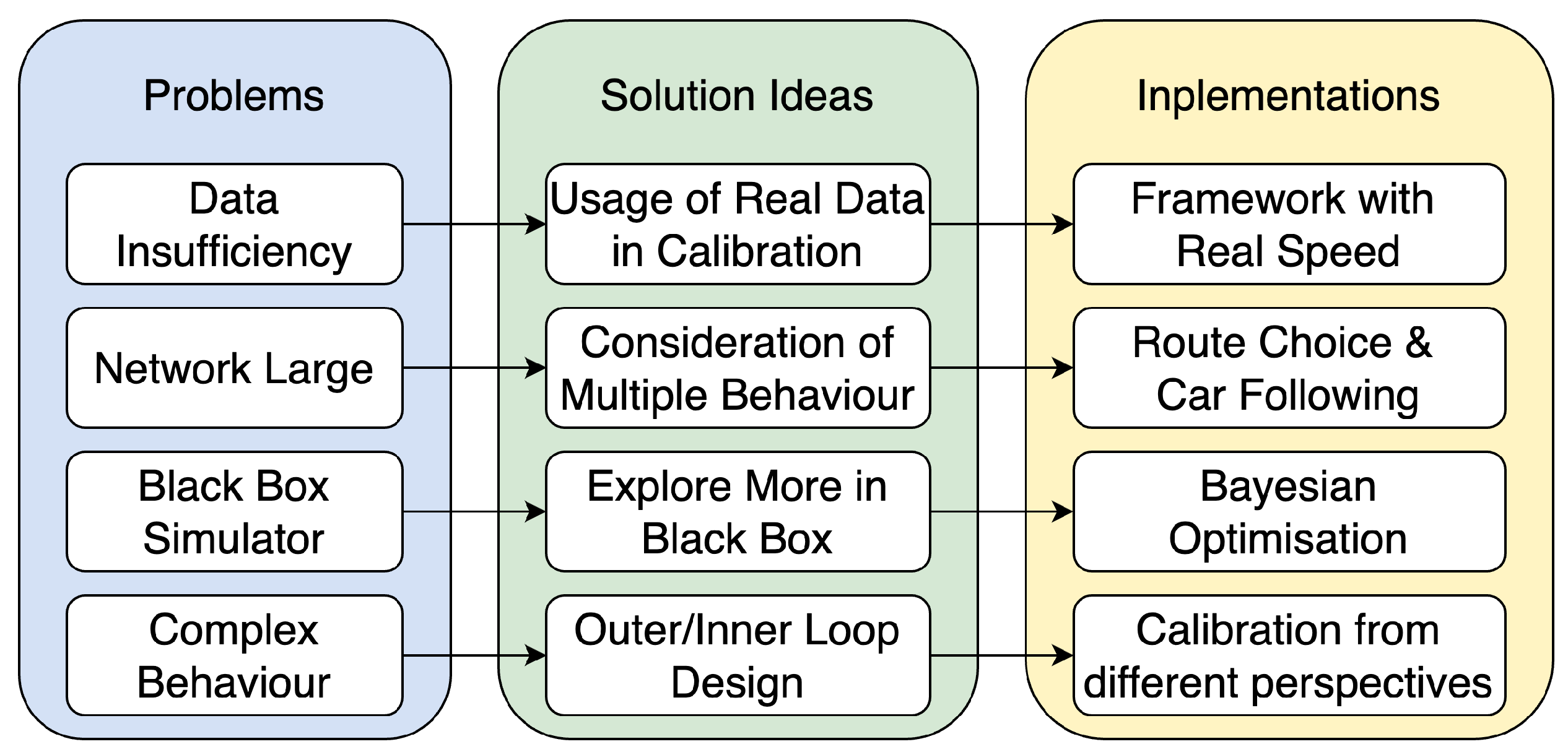
• Data Insufficiency: We have limited real data compared to the large-scale network (in the case of the Bay Area, the simulator has a route network composed of 547,697 edges and 223,328 nodes), which encompasses the average traveling speed of each link and the flow amount of part of the link in different time periods. Compared to the traditional car-following parameter calibration [11], we do not have vehicle-level trajectory data or real-time speed data.
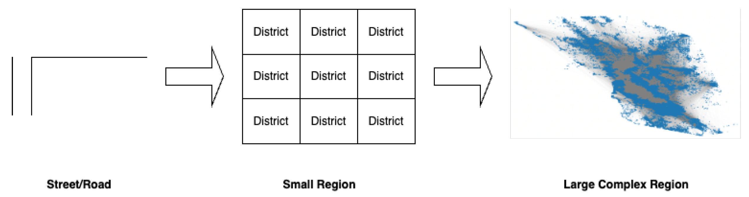
• Large Network Scale: Due to the large scale of the simulator, the traffic condition will be much more complex compared to the district- or city-level calibration [9,14] researchers conducted before. The growing complexity results in the advanced design of exploring the black box structure in the traffic simulator.

Table 1. Summary of the literature on micro-simulation car-following calibration.

Authors	Network Scope	Measurement	Calibration Algorithm
Balakrishna et al. [15]	2564 segments, 400+ OD	Flow	SPSA
Lee and Ozbay [16]	Small scale	Flow; speed; headway	Bayesian sampling; E-SPSA
Aghabayk et al. [17]	All scale (no experiment)	NA	Evolutionary algorithm
Azevedo et al. [18]	Urban motorway	Flow; speed; acceleration; deceleration; headway	Kriging, WSPSA
Chiappone et al. [19]	A22 Freeway	Speed–density relationship	Genetic algorithm
Jiménez et al. [20]	Pereira, Colombia (small scale)	GoF	Genetic algorithm
Markou et al. [21]	Naples, Italy (small scale)	Distance; speed	SPSA
Schultz and Sokolov [22]	POLARIS (small scale)	Travel time	Bayesian optimization; active subspace; deep neural networks

summarizes a small sample of the past car-following calibration work. In the literature, the majority of the past work has used the trajectory data or real-time speed data of individual vehicles as real data. The use of link-level data as ground truth real data, such as average link travel time data, has been less explored. In addition, most past work has considered small networks with limited node and edge scales. The network scale in the previous work is not in the same order of magnitude as what we need to tackle.

Building on the observations and requirements outlined earlier, we introduce the DRBO framework, which integrates route choice behavior calibration with car-following parameter tuning. This framework is designed to iteratively refine both aspects, improving the accuracy of large-scale traffic simulations. Figure 1 provides an overview of the calibration process, showing how network data and typical day demand feed into the routing and parameter calibration steps. To clarify its interaction with the simulator, it is important to note that the simulator plays a central role in both calibration stages. During car-following parameter calibration, the simulator runs multiple iterations to compare simulated and observed traffic speeds, adjusting parameters accordingly through Bayesian optimization. In the route choice calibration step, the simulator evaluates travel times based on previous routing decisions, allowing the model to update routing behavior dynamically. The results from these simulations continuously feed back into the calibration loop, ensuring that the framework minimizes discrepancies between simulated and real-world traffic patterns. By making these connections explicit, Figure 1 can better illustrate the iterative process and the simulator’s role in refining model accuracy.

As for the contributions of the paper, we need to mention that DRBO is the first framework to undertake the calibration of the regional scale transportation network. Based on its characteristics, the framework designs the iterative method for calibration, using Bayesian optimization or route adjustment at each step of the iteration. It innovatively integrates the techniques in black box optimization and travel behavior modeling. Besides the technique design and promising experiment results, we also provide insightful discussion for the iterative structure, which will be presented in the later section.

The structure of this article is laid out as follows: Section 2 provides some work related to this paper. Section 3 dives into two key components in the calibration framework: the day-to-day real-world routing calibration algorithm and the Bayesian optimization approach calibrating the car-following parameters. In addition, we also show the mathematical intuition behind the iterative framework design. Section 4 provides the experiment results of calibration.

2. Literature Review

In this part, we first review how researchers carried out calibration in traffic simulators. Motivated by the review, we briefly introduce the technical components in our calibration framework and provide a review of these technical details.

2.1. Simulation Calibration in Transportation Simulator

Calibration in transportation simulation systems involves a systematic process of refining model parameters to align simulation outputs with real-world observations.

One type of the work [11,23,24] focuses on the detailed data of individual cars (detailed speed data or location data) and considers the calibration problem in relatively small regions. Since the road and region structure is not hard to identify under these settings, the core of calibration is cast into solving an analytical optimization problem, in which the decision variables are car-following model parameters and the objective function usually characterizes the difference between empirical vehicle movements and their simulated correspondences. Researchers derive various algorithms in numerical optimization to solve the calibration optimization problem. These works [25,26,27] indeed gave a comprehensive understanding and benchmark in the traditional car-following model calibration. However, the analytical expression of the optimization problem is hard to derive on a much more complex network. It motivated the appearance of the literature combining the black box system with the calibration problem.

Considering the black box property of the simulation system, various works used black box optimization techniques for simulation calibration. The methodologies include Bayesian optimization [8,9], simultaneous perturbation stochastic approximation (SPSA) [15], etc. Among them, Bayesian optimization is one of the most powerful tools, which enhances the sampling procedure using the Gaussian Process as the surrogate model of the simulation system. The key steps of Bayesian optimization include building a surrogate model based on current observation, choosing the next sample points according to the minimization of the acquisition function, and updating the model after each iteration until convergence. However, in the literature summarized in Table 1, people mainly considered the car-following and lane-changing parameters as factors influencing the output of speed. They did not consider how the route choice behavior influences the mobility system. Their thoughts are reasonable in small regions because different route choices may lead to little change to the average travel time on the edge. In contrast, for regional-level transportation networks, how the vehicles choose their route makes a great impact on simulator output.

The prevalent literature review motivates us to think about how to conduct calibration on the large-scale transportation network. Readers can refer to Figure 2 for a network-size development visualization. In our work, we integrate the routing algorithm and parameter calibration in the DRBO calibration framework. We will give a comprehensive review of the routing behavior and the Bayesian optimization used in parameter calibration.

2.2. Routing Behavior

Factors in Routing Problem

In this part, we first review the modeling framework of the routing problem, which is highly related to the factors influencing the route choice. That is, how an individual vehicle chooses their route based on OD information and their traveling experience.

One of the most common types of routing behavior is based on finding the shortest path [28] between a source and destination. Dijkstra’s algorithm [29] is a classical algorithm that calculates the shortest path based on edge weights (e.g., travel time, distance) in a graph representation of the road network. This algorithm is efficient for static environments but may not capture real-time traffic conditions. To account for dynamic traffic conditions, dynamic routing algorithms [30] continuously update and adapt routes based on real-time data. This includes algorithms that use traffic flow information, such as Traveling Salesman Problem (TSP) heuristics or A⋆ search with dynamic edge costs that incorporate current traffic speeds.

Specifically, in microscopic simulations, each vehicle is represented as an intelligent agent that makes routing decisions based on its own experience. Agents can use the shortest path algorithm or dynamic routing algorithm to perform routing as mentioned above. In addition, modern agent-based routing behavior incorporates advanced navigation features [31], such as real-time rerouting based on traffic incident alerts, predictive modeling of traffic patterns, or considering alternative modes of transportation (e.g., public transit, ridesharing) to optimize multimodal routes [32].

2.3. Routing Problem as Game

In this part, we see the routing problem as a game and review the relevant literature about this topic.

We first introduce the dynamic traffic assignment (DTA) problem, which is different but closely related to the routing problem [33,34]. The goal of the DTA is to simulate how travelers dynamically choose routes and departure times based on evolving information, aiming to predict traffic flow and congestion levels accurately. The departure times were the same for different days to ensure consistency in comparing the travel times across different iterations. One of the common approaches is the user equilibrium (UE) method [35] (calculating the route choice behavior that all of the agents do not have the intention to change their path). From the theoretical perspective, the DTA result can be seen as the limiting behavior of the day-to-day route choice [36].

Secondly, we introduce the mean field game (MFG) theory, which has emerged as a powerful framework for studying dynamic routing in transportation systems by modeling the collective behavior of a large population of vehicles or travelers [37]. In the context of transportation, MFGs allow for the analysis of how individual routing decisions impact overall traffic flow and congestion dynamics. By considering the interactions among a large number of agents, each agent makes routing choices based on their own objectives and perceptions of traffic conditions in a learning framework [38].

2.4. Bayesian Optimization

Bayesian optimization (BO) has garnered significant attention in the literature due to its effectiveness in optimizing complex and expensive-to-evaluate functions, with applications ranging from hyperparameter tuning in machine learning to experimental design and sequential decision-making [39]. A prominent aspect of BO is its ability to leverage probabilistic models, typically Gaussian Processes, to build surrogate models of the objective function and guide the search towards promising regions of the parameter space. Numerous studies have explored different aspects of BO, including strategies for handling high-dimensional and noisy optimization problems [14], enhancing computational efficiency through parallelization and efficient acquisition function optimization [40], and integrating BO with deep learning methods for scalable and robust optimization. Overall, the extensive literature on Bayesian optimization reflects its versatility and applicability across various domains, providing valuable insights into the theoretical foundations, algorithmic developments, and practical implementations of this powerful optimization methodology.

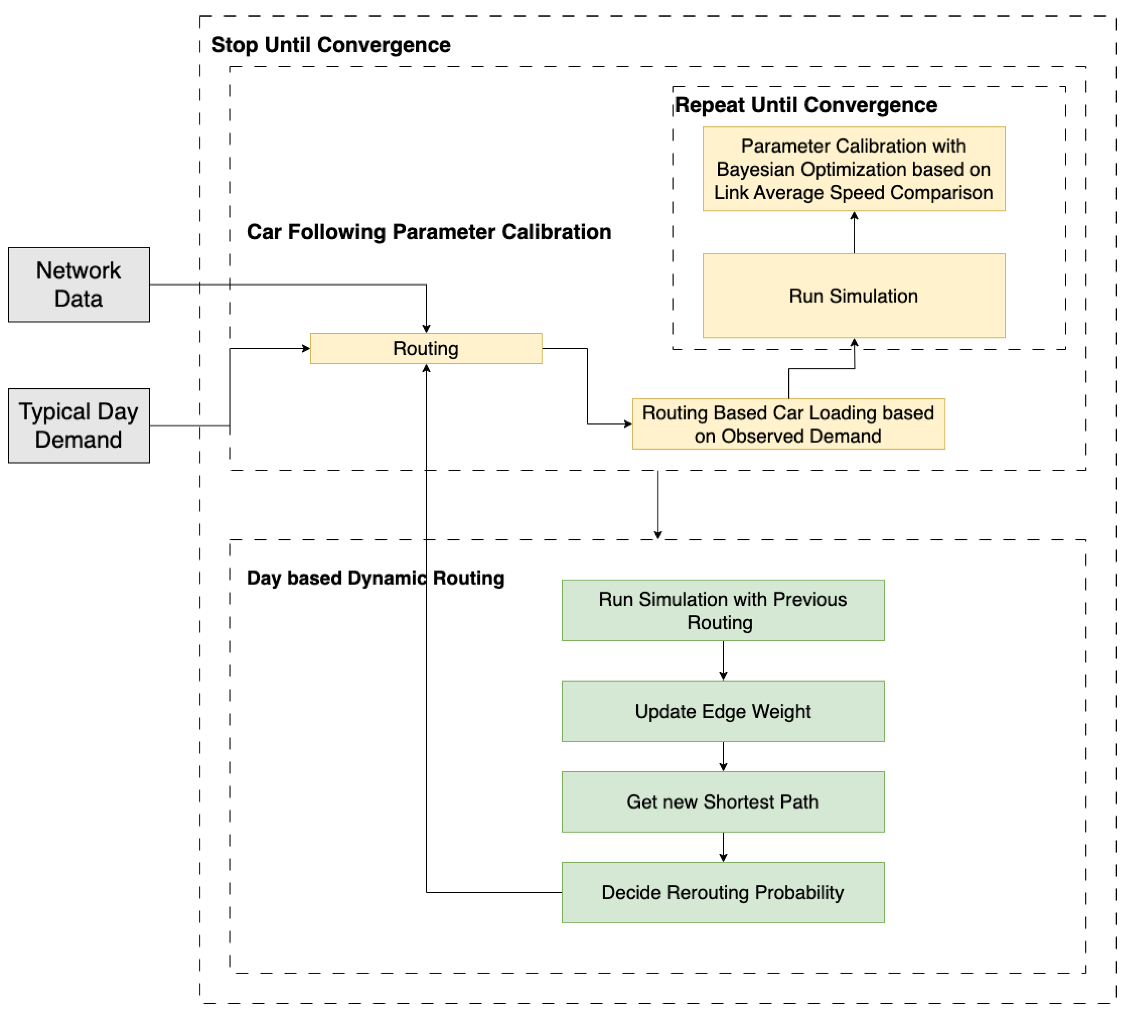
3. Calibration Framework

3.1. Framework Contents

In the calibration process we designed, we use a double-iterative two-stage calibration approach. In each outer iteration, we first simulate individual road segments based on the real traffic flow in the time period. We output the average speed of each segment and define the minimization objective function as the difference between the average simulated speeds for all segments at all times and the real data. We then use black box optimization to calibrate and obtain the optimal car-following parameters based on the output. Secondly, based on the structure of our OD demand (demand of a typical day, which refers to a day with average travel patterns, especially for commuting, that represents normal behavior), we update the routes day by day following the route choice pattern which will be introduced in the next subsection.

We need to note that in the first stage of each outer iteration, before loading vehicles on specific edges, we should first learn the flow distribution pattern during the simulated time period by the last simulation output of the former outer iterative. Then, we follow this pattern to distribute the vehicles onto edges and perform Bayesian optimization sequentially.

To better illustrate the motivation of our Figure 2, we present the following Figure 3 to show the mapping of difficulties in regional scale simulator calibration and our corresponding solution. It illustrates the mapping between key challenges in regional scale simulator calibration and the corresponding solutions adopted in our framework. The challenges include data insufficiency, large-scale network complexity, the black box nature of the simulator, and intricate behavioral interactions. To address these, we leverage real-world data for calibration, incorporate diverse behavioral considerations, explore optimization strategies tailored for black box systems, and implement a structured outer/inner loop design. These solution ideas are further implemented through a framework integrating real speed data, route choice and car-following calibration, Bayesian optimization, and multi-perspective calibration strategies. This structured approach ensures that the calibration process remains robust, scalable, and computationally efficient.

The description of the simulator we took as an example to perform large-scale calibration can be found in Appendix A, which provides details on LPSim, the discrete time-driven simulation platform employed in our study. LPSim enables large-scale microsimulation for both vehicles and aircraft, utilizing a parallelized GPU implementation to handle networks with hundreds of thousands of nodes and millions of trips efficiently. It was tested on the San Francisco Bay Area road network, consisting of 547,697 edges and 223,328 nodes, with various road classifications such as local streets, arterials, highways, and freeways. The Appendix A also describes key vehicle dynamics, including the Intelligent Driver Model (IDM) for acceleration behavior and mandatory lane change processes governed by mathematical formulations. In the following subsections, we introduce two key components of the DRBO calibration framework: car-following model calibration and dynamic route choice adjustment.

In the following subsections, we separately introduce two key parts of the DRBO framework.

3.2. Calibration Part A—Route Choice Behavior

In this section, we explain how we calibrate route choice behavior in our framework Figure 1. In real-world traffic, many factors affect route choice, such as the shortest path, estimated travel time, and past travel times. Since multiple vehicles make decisions at the same time, routing becomes a dynamic process. Our goal is to mimic real-world behavior while keeping the calibration process efficient. Since the demand reflects a typical day, we follow the calibration approach outlined in Algorithm 1.

In each iteration, the vehicle changes the route choice with probability computed by the function related to its travel time in the days before. This strategy [41] seeks to imitate the navigation system in the real-world scenario. Several studies [42,43,44,45] also confirm the idea in [41] that the difference between travelers’ estimated travel costs and their expected travel costs plays a key role in rerouting behavior. Besides the modeling factor, this rerouting framework is also lightweight to implement compared to the mean-field game modeling introduced in Section 2, which requires extensive computation and evolution of the system in the learning process.

Algorithm 1 Routing Calibration Procedure in Outer Loop-Agent Level w

Input: t (Current Inner Loop Iteration), $\mathcal{G}$ (Graph of the network with edges e and nodes n), $v_{free}$ (Free Flow Speed) Parameter: $\alpha$ (Scaling factor for rerouting probability sensitivity), $ϵ$ (Small positive constant to ensure numerical stability), $R_{t-1}$ (Travel Path of the agent on day $t-1$), $T{T}_{e_i}(t-1)$ (Travel Time on edge $e_i,i\in \{1,2,\dots ,N\}$ at day $t-1$ for all routes connecting the agent-specific OD pair in an hour), $T{T}_{t-1}$ (Travel time of the agent on day $t-1$) Output: Route ($\mathcal{R}$) based on previous experience and rerouting criteria If $t=0$: Initialize the parameters $\alpha$ and $ϵ$ as constants. Determine $\mathcal{R}$ using the shortest path algorithm. Otherwise ($t>0$): Determine the gap $\Delta =T{T}_{t-1}-T{T}_{t-2}$. Calculate the reroute probability: $$p(\Delta )=\left\{\begin{array}{cc}{\displaystyle \frac{{\alpha }_t{(\Delta )}^3}{{(\Delta )}^3+ϵ}}\hfill & \mathrm{if}\Delta >0\hfill \\ 0\hfill & \mathrm{if}\Delta \le 0\hfill \end{array}\right.$$ Reroute based on the reroute probability. Return the route $\mathcal{R}$.

To be specific, the framework above captures the route change behavior by calculating the gap $\Delta$, which reveals the gap of the agent travel time with the average of the travel time of other route choices connecting the same OD pair on the day (inner iteration) $t-1$. We point out that when $\Delta <0$, the vehicle concludes that it is a great path choice that allows the shortest path, and the agent tends not to change the choice. When $\Delta >0$ and it increases, the probability of changing the route increases because $p(\Delta )$ is an increasing function. This mechanism imitates the role of the navigator in the transportation area, which gives decision advice to agents based on previous observations. $p(\Delta )$ is used in Algorithm 1 to determine the probability of rerouting when the travel time gap $\Delta$ between consecutive iterations is positive, influencing whether an agent switches to an alternative route.

Remark: The probability function $p(\Delta )$ does not explicitly incorporate additional factors such as weather or incident-related disruptions, and the travel-time metric can implicitly capture recurring congestion patterns, driver delays, and certain nonrecurrent events that affect average daily travel. For instance, if an incident or adverse weather frequently causes a significant delay on a specific route, the resulting increase in travel time would raise $\Delta$, subsequently increasing the probability that a traveler would switch routes in the next iteration. We acknowledge, however, that truly short-term or unexpected disruptions might not be perfectly reflected by a purely day-to-day travel time difference.

3.3. Calibration Part B—Car-Following Parameter

We use the Intelligent Driver Model (IDM) (1), a classical car-following parameter in the simulator. It delineates the acceleration behavior of vehicles for the usage of updating vehicle locations at each time step. In experiments, we find that different car-following parameter settings have a great impact on the simulation output. Therefore, it is essential to calibrate the parameters $a,b,s_0,\delta$ in the IDM model.

$$\dot{v}=a\left(1-{\left({\displaystyle \frac{v}{v_o}}\right)}^{\delta }-{\left({\displaystyle \frac{s_o+Tv+\frac{v\Delta v}{2\sqrt{ab}}}{s}}\right)}^2\right)$$

(1)

The motivation for the parameter calibration method we propose is the lack of individual driver real data in the large transportation system. We can only use the flow data of several roads, the OD data of the typical day, and the real average speed of the roads.

Based on the condition above, we load the known flow amount based on the vehicle density distribution obtained in the simulation before. Then, by implementing Bayesian optimization (due to the black box property of the simulator), we calibrate the parameters of the system iteration by iteration. For the explanation of density loading and algorithm framework, readers can refer to Figure 4 and Algorithm 2. After the overall introduction, we explain how and why we use Bayesian optimization here for parameter calibration.

The objective function of our parameter calibration optimization problem takes the following formulation (2), where $a,b,s_0,\delta$ refer to the parameters we want to calibrate, $v_i(a,b,s_0,\delta )$ is the average speed generated by the simulator on link i, and $v_i$ is the real speed by the Uber data.

$$minf(a,b,s_0,\delta )=\sum _{i=1}^N{\parallel v_i(a,b,s_0,\delta )-v_i\parallel }^2$$

(2)

We are unable to explicitly formulate Equation (2) in terms of the variables $a,b,s_0,\delta$. One possible approach is to exhaustively sample a wide range of parameter combinations and select the one that minimizes the objective function. However, this method is computationally expensive. To address this, researchers have developed Bayesian optimization, which provides a more efficient approach by leveraging a surrogate model and an acquisition function to guide the selection of parameter values. This approach enables more informed and targeted sampling, reducing computational overhead while improving optimization efficiency. For further details on Bayesian optimization, readers may refer to the tutorial in [39] and its applications in transportation studies [9].

Algorithm 2 Parameter Calibration for link e in the time interval $[a,b]$ at the t -th outer loop

Initialization-a: Flow density distribution at final simulation run at outer loop $t-1$ Initialization-b: Standard flow amount for link e at the time interval $[a,b]$ Initialization-c: Load the agents based on initialization a and b Optimization: Using Bayesian Optimization to iteratively update the parameters in the simulation system. (Surrogate Model: Gaussian Process; Acquisition function: Expectation Improvement)

To further match flow count with realistic observation, suppose for agent i that there are several paths from the origin O to destination D; there are n paths with flow $d_j,j\in \left[m\right]$, and the ground truth flow is $g_j,j\in \left[m\right]$ (suppose they follow the descent ranking in the term $\left.g_j-d_j\right)$.

$$g_1-d_1\ge g_2-d_2\ge \cdots \ge g_m-d_m$$

(3)

To facilitate the choice model, we first perform a shift to make them all positive, and the sequence is calculated by

$$s_j=g_j-d_j+max\left(d_m-g_m,0\right)$$

(4)

The agent choice probability distribution is

$$p_j={\displaystyle \frac{s_j}{{\sum }_{i=1}^m{s}_j}}$$

(5)

Based on the route choice probability distribution, we further reroute people to certain routes to lower the flow count gap between simulation and real-world observations.

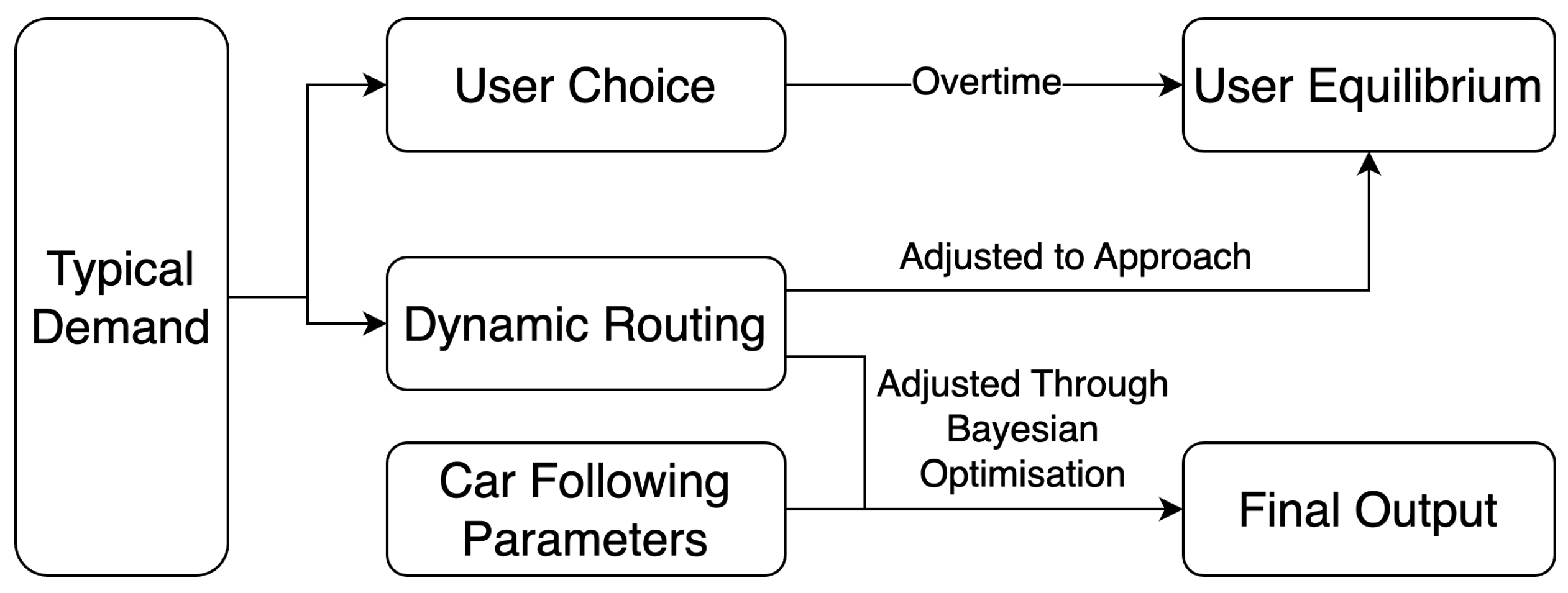
3.4. Further Discussion—Intuition Behind Framework Design

We will show the experiment results in Section 4. Before this, we provide some further discussions about the intuition designing the framework. This is shown in Figure 5.

The framework design is motivated by the typical day demand. It is proved that for a day-to-day routing game, agents can adjust their route choice based on the utility function and will finally converge to the so-called user equilibrium [36]. Based on this background, there are two questions that come to mind:

• Is the user equilibrium the best route choice for the simulator calibration?
• Can we use the route choice adjustment strategy to approach the ideal routing strategy which minimizes the gap of simulator output and the real data?

The answer to the first question is “No”. This is because the UE acts as a limiting behavior, but the real data are estimated on a specific day or are the average of several countable days. The answer to the second question is yes. This is due to the typical day demand structure. We believe that vehicles have some adaptation to the traffic condition which can be approximated by adjusting route choice day by day in the inner loop.

Based on the answers above, we combine the car-following dynamic and route choice in a subsequent way, conducting two aspects of calibration independently and iteratively to obtain the final simulator calibration results.

4. Experiment

4.1. Data Source

4.1.1. Demand Data

In this research, we engaged in a comprehensive collaborative effort by leveraging data from the San Francisco County Transportation Authority (SFCTA) [46]. Our analysis was informed by the San Francisco Chained Activity Modeling Process (SF-CHAMP) [47], a sophisticated modeling system that projects transportation patterns across the nine counties of the San Francisco Bay Area. The San Francisco Bay Area is a diverse metropolitan region in Northern California, with people of different travel patterns. Utilizing SF-CHAMP 6, which draws on observed travel behaviors and socio-economic data from local residents, this system provides critical insights into the region’s transportation infrastructure and assists in urban planning.

The core of our analysis was a detailed dataset of trips reflecting a typical weekday free of significant events or seasonal variations [48]. Each record in the dataset was meticulously categorized by origin, destination, transportation mode, and other essential attributes. Our focus was specifically on car trips, distinguishing between single-occupant vehicles (SOVs), two-occupant vehicles (HOV 2), and vehicles with three or more occupants (HOV 3+). After applying these classifications, our analysis encompassed 17.8 million car trips, which constituted 80.4% of the total dataset. This subset served as a robust foundation for our examination of vehicular movement patterns, shedding light on dominant vehicle flows and their broader implications for traffic management and urban development.

4.1.2. Flow Data

We obtained observed flow counts from various sources, detailed as follows:

• F&P: Counts that were collected and passed to us.
• SFMTA: Counts obtained from tube detectors.
• Freeway performance measurement system (PeMS): 30 s loop detector data in California [49].
• CMP’s “multimodal counts data”: Our dataset is segmented into several time periods:

  –

  Early Morning (EA) from 3:00 a.m. to 6:00 a.m.;

  –

  Morning Peak (AM) from 6:00 a.m. to 9:00 a.m.;

  –

  Midday (MD) from 9:00 a.m. to 3:30 p.m.;

  –

  Afternoon Peak (PM) from 3:30 p.m. to 6:30 p.m.;

  –

  Evening (EV) from 6:30 p.m. to 3:00 a.m.

These sources provide a comprehensive temporal spread and diverse measurement methods, enhancing our dataset and its utility in analyzing traffic patterns.

4.1.3. Link Average Speed Data

To validate the traffic microsimulator, we compare the outputs from LPSim [50] with Uber Movement average speed distributions [2] for specific time slices. The Uber Movement data were chosen because they provide high-resolution and reliable traffic speed data derived from actual vehicle movements, making them an ideal benchmark for validating simulation models. The dataset is well suited to the regional scale of the San Francisco Bay Area network and has been widely used in transportation research, ensuring credibility and comparability with other studies.

For this study, we utilized Q2 Uber Movement data from 2019 [2], covering 95,510 edges, which represents 17% of the total edges in the San Francisco Bay Area network. This subset of the network was selected due to its high data availability and its representation of key traffic corridors in the region.

These characteristics of the Uber Movement data provide a robust foundation for validating the outputs of LPSim, as the data capture both spatial and temporal traffic variations across a large-scale network.

4.2. Practical Error Measure

In the large-scale simulator, it is hard to minimize Equation (2) to a great extent for the system is rather complex. In our experiment, we construct the distribution by link travel speed and calculate the Wasserstein distance of the simulator output distribution with the true distribution.

The Wasserstein distance [51], also known as the Earth Mover’s Distance, is a metric used to quantify the difference between two probability distributions over a given metric space. It is based on the idea of the minimum cost required to transform one distribution into the other by moving the probability mass. Specifically, the cost is determined by the amount of mass moved and the distance it is moved, aiming to minimize this total cost. The Wasserstein distance is particularly useful in fields like machine learning, image processing, and economics as it provides a meaningful way to compare distributions that takes into account both the geometry and the inherent structure of the data.

Let $(M,d)$ be a metric space that is a Polish space. For $p\in [1,+\infty ]$, the Wasserstein p-distance between two probability measures $\mu$ and on M with finite p-moments is

$$W_p(\mu ,\nu )=\underset{\gamma \in \Gamma (\mu ,\nu )}{inf}{\left(E_{(x,y)\sim \gamma }d{(x,y)}^p\right)}^{1/p}$$

(6)

where $\Gamma (\mu ,\nu )$ is the set of all couplings of $\mu$ and $\nu ;W_{\infty }(\mu ,\nu )$ is defined to be ${lim}_{p\to +\infty }{W}_p(\mu ,\nu )$ and corresponds to a supremum norm. A coupling $\gamma$ is a joint probability measure on $M\times M$ whose marginals are $\mu$ and $\nu$ on the first and second factors, respectively. That is, for all measurable $A\subset M$ a coupling fulfils

$$\begin{array}{cc}\hfill {\int }_A{\int }_M\gamma (x,y)\mathrm{d}y\mathrm{d}x& =\mu \left(A\right),\hfill \\ \hfill {\int }_A{\int }_M\gamma (x,y)\mathrm{d}x\mathrm{d}y& =\nu \left(A\right).\hfill \end{array}$$

Furthermore, we checked the correlation between the simulated flow and the observed flow to check the convergence of the algorithm.

$$r={\displaystyle \frac{\sum \left(x_i-\overline{x}\right)\left(y_i-\overline{y}\right)}{\sqrt{\sum {\left(x_i-\overline{x}\right)}^2·\sum {\left(y_i-\overline{y}\right)}^2}}}$$

(7)

4.3. Experiment Results

We list several experiment results below by visualizing the distribution of link average travel speed output by Uber Movement data and the simulator. We begin by comparing the flow counts, followed by a detailed examination of the speed distributions in both the simulated and observed data. Lastly, we analyze the fundamental diagram to assess the overall validity and coherence of the approach.

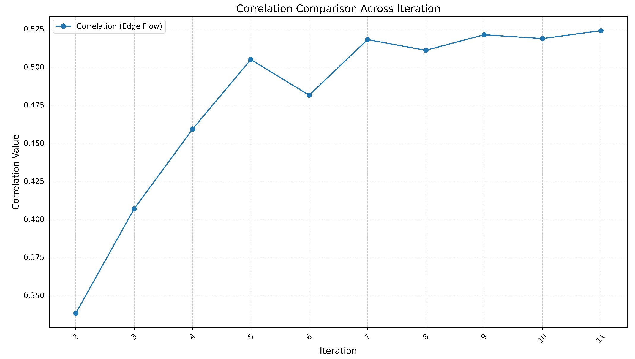
4.3.1. Flow Correlation

We checked the correlation between our flow count and observed flow count as listed in Section 4.2. The iterative improvement in the correlation between simulated and observed edge flow is presented in Figure 6. This figure demonstrates the convergence behavior of the calibration framework across iterations. The correlation values, initially around 0.35 in the first iteration, steadily improve with each subsequent iteration, reaching approximately 0.525 after the 10th iteration. This progressive increase reflects the effectiveness of the double-iterative two-stage calibration process in aligning simulated traffic flow with real-world observations.

The increase in correlation can be attributed to the iterative refinement of both the car-following parameters and the route choice behavior. The use of Bayesian optimization in the outer loop efficiently adjusts the car-following parameters to minimize discrepancies between simulated and observed speeds. Simultaneously, the inner loop focuses on rerouting vehicles based on day-to-day travel time differences ($\Delta$), improving the alignment of simulated flows with observed data.

The slight stabilization of the correlation values beyond the sixth iteration suggests diminishing returns from further iterations. This plateauing effect highlights the potential for additional refinements, such as incorporating more detailed real-world data or optimizing the rerouting mechanism to better capture edge-specific variations in traffic flow.

4.3.2. Speed Distribution Comparison

After the correlation becomes steady, we compare the differences between simulated and observed average speeds, which is illustrated in Figure 7. This provides a validation of the calibration framework during the time period from 3 a.m. to 4 a.m. as an example (the full day result is in Figure 8). The Uber Movement data serve as a benchmark, representing real-world conditions with a mean speed of 27.55 miles per hour (MPH) and a standard deviation of 9.26 MPH. The simulated distribution demonstrates a close alignment, with a mean of 27.43 MPH and a standard deviation of 9.50 MPH. The Wasserstein distance between the two distributions is 1.17, indicating a reasonable match between simulated and observed data.

The experiment validates the effectiveness of the proposed calibration framework in replicating real-world traffic patterns for a large-scale transportation network. However, the limitations of flow data and the scale of the demand introduce uncertainties in the simulation results. The current study extends it to the full-day time interval, from 00 a.m. to 11:59 p.m. The satisfactory agreement between the simulated and observed speed distributions in Figure 8 underscores the efficiency of the framework. Nevertheless, the observed variations highlight the need to incorporate additional factors, such as weather conditions, incidents, and other non-recurring disruptions, to improve model fidelity. The ongoing development of the framework will address these limitations, aiming to provide a comprehensive and reliable tool for large-scale traffic simulation and urban transportation planning.

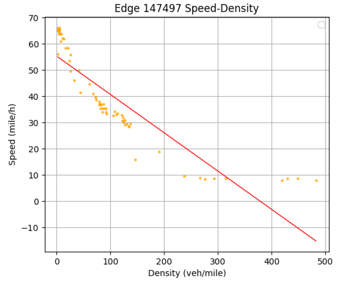
4.3.3. Link Fundamental Diagram (FD)

In addition to the analysis above, we also plotted the fundamental diagram for a randomly selected link in the network. To further evaluate the calibration framework, we plotted the fundamental diagram for Edge 147497, as shown in Figure 9, which represents the flow–density relationship. We also plotted the speed–density relationship in Figure 10. This analysis provides insights into the traffic dynamics for the selected link, highlighting key parameters such as free-flow speed, capacity, and jam density.

From the flow–density diagram:

• The free-flow region is observed at densities below approximately 250 veh/mile, where flow increases almost linearly with density. This region reflects uncongested traffic conditions, where vehicles can travel at near-optimal speeds.
• The capacity point occurs at a density of approximately 250 veh/mile, with a maximum flow of around 4500 veh/h. This corresponds to the critical density, indicating the maximum throughput achievable on the link.
• Beyond this point, in the congested region, flow decreases as density increases. This indicates over-saturated traffic conditions, where vehicle interactions and reduced speeds dominate.

The results align well with theoretical expectations of traffic flow dynamics. The parabolic shape of the curve confirms that the simulator effectively captures the nonlinear relationship between flow and density, consistent with established traffic flow theories. Deviations in the congested region suggest the influence of external factors or stochastic variations in vehicle behavior.

These findings emphasize the accuracy of our simulation approach in replicating real-world traffic conditions at the link level. The ability to derive traffic parameters, such as free-flow speed, capacity, and jam density, validates the robustness of the calibration process. Moreover, the fundamental diagram provides a critical perspective on the intricate relationship between flow and density, serving as a foundation for network-level analysis.

5. Conclusions

This paper introduces DRBO, a calibration framework for the large-scale traffic simulator. Unlike traditional calibration methods, DRBO integrates the route choice behavior update and parameter calibration via Bayesian optimization, ensuring efficient calibration of the large system.

The key innovation of DRBO is its framework design, which admits outer loop iterations and inner loop iterations. In each outer loop, DRBO calibrates the system parameter by Bayesian optimization at first and performs the route choice update according to reasonable criteria in another inner iteration. The motivation of this approach is the typical day demand structure and the consideration of system factors (car-following dynamic, route choice behavior). The experimental results on the large-scale simulator LPSim show its superior performance.

The experiment presented in this study is centered on the San Francisco Bay Area, leveraging the region’s rich data availability, including SFCTA trip demand and Uber Movement speeds. However, the proposed methodology, DRBO’s two-stage framework combining dynamic routing and Bayesian optimization, is inherently transferable and not restricted to this specific region. Its applicability extends to any context where (i) link-level data are accessible for calibration and (ii) the network can be represented within a compatible microscopic simulation environment.

Future enhancement directions of the DRBO calibration framework lie in two fold.

Firstly, a straightforward direction is to extend our current work to a larger-scale network. The extension is not trivial. As the scale becomes super large, we need to balance the trade-off between calibration quality and computation speed using the hardware and data structures. When the calibration is super time-consuming, it will lose its original value to a great extent.

Secondly, from the BO perspective, there has been an open problem about how to design a unified high-dimensional efficient Bayesian optimization algorithm. In recent years, different researchers have proposed different approaches combined with domain knowledge including the transportation area [9]. However, the idea in [9] seems to fail in our calibration task because we do not have a physical surrogate model in the large-scale system. It is natural to think about the following question: if the amount of parameters in our simulation system is large, how do we use the power of Bayesian optimization efficiently and tackle the problems in the high-dimensional settings?

References

1. Behrisch, M.; Bieker, L.; Erdmann, J.; Krajzewicz, D. SUMO–simulation of urban mobility: An overview. In Proceedings of the SIMUL 2011, the Third International Conference on Advances in System Simulation, ThinkMind, Barcelona, Spain, 23–29 October 2011. [Google Scholar]
2. Yedavalli, P.; Kumar, K.; Waddell, P. Microsimulation analysis for network traffic assignment (MANTA) at metropolitan-scale for agile transportation planning. Transp. A Transp. Sci. 2021, 18, 1278–1299. [Google Scholar] [CrossRef]
3. Jiang, X.; Agerup, J.F.; Tang, Y. Benchmarking and Preparing LPSim for Scalability on Multiple GPUs; University of California: Berkeley, CA, USA, 2023. [Google Scholar]
4. Archetti, C.; Speranza, M.G.; Weyland, D. A simulation study of an on-demand transportation system. Int. Trans. Oper. Res. 2018, 25, 1137–1161. [Google Scholar] [CrossRef]
5. Esser, J.; Schreckenberg, M. Microscopic simulation of urban traffic based on cellular automata. Int. J. Mod. Phys. C 1997, 8, 1025–1036. [Google Scholar] [CrossRef]
6. Huang, J.; Cui, Y.; Zhang, L.; Tong, W.; Shi, Y.; Liu, Z. An overview of agent-based models for transport simulation and analysis. J. Adv. Transp. 2022, 2022, 1252534. [Google Scholar] [CrossRef]
7. Goyal, R.; Reiche, C.; Fernando, C.; Serrao, J.; Kimmel, S.; Cohen, A.; Shaheen, S. Urban Air Mobility (UAM) Market Study; NASA Technical Reports Server (NTRS): Washington, DC, USA, 2018; Volume 30. [Google Scholar]
8. Sha, D.; Ozbay, K.; Ding, Y. Applying Bayesian optimization for calibration of transportation simulation models. Transp. Res. Rec. 2020, 2674, 215–228. [Google Scholar] [CrossRef]
9. Tay, T.; Osorio, C. Bayesian optimization techniques for high-dimensional simulation-based transportation problems. Transp. Res. Part B Methodol. 2022, 164, 210–243. [Google Scholar] [CrossRef]
10. Park, B.; Qi, H. Development and Evaluation of a Procedure for the Calibration of Simulation Models. Transp. Res. Rec. 2005, 1934, 208–217. [Google Scholar] [CrossRef]
11. Li, L.; Chen, X.M.; Zhang, L. A global optimization algorithm for trajectory data based car-following model calibration. Transp. Res. Part C Emerg. Technol. 2016, 68, 311–332. [Google Scholar] [CrossRef]
12. Ho, M.C.; Lim, J.M.Y.; Chong, C.Y.; Chua, K.K.; Siah, A.K.L. High dimensional origin destination calibration using metamodel assisted simultaneous perturbation stochastic approximation. IEEE Trans. Intell. Transp. Syst. 2023, 24, 3845–3854. [Google Scholar] [CrossRef]
13. Monteil, J.; O’Hara, N.; Cahill, V.; Bouroche, M. Real-time estimation of drivers’ behaviour. In Proceedings of the 2015 IEEE 18th International Conference on Intelligent Transportation Systems, Gran Canaria, Spain, 15–18 September 2015; IEEE: New York, NY, USA, 2015; pp. 2046–2052. [Google Scholar]
14. Malu, M.; Dasarathy, G.; Spanias, A. Bayesian optimization in high-dimensional spaces: A brief survey. In Proceedings of the 2021 12th International Conference on Information, Intelligence, Systems & Applications (IISA), Chania Crete, Greece, 12–14 July 2021; IEEE: New York, NY, USA, 2021; pp. 1–8. [Google Scholar]
15. Balakrishna, R.; Antoniou, C.; Ben-Akiva, M.; Koutsopoulos, H.N.; Wen, Y. Calibration of microscopic traffic simulation models: Methods and application. Transp. Res. Rec. 2007, 1999, 198–207. [Google Scholar] [CrossRef]
16. Lee, J.B.; Ozbay, K. New calibration methodology for microscopic traffic simulation using enhanced simultaneous perturbation stochastic approximation approach. Transp. Res. Rec. 2009, 2124, 233–240. [Google Scholar] [CrossRef]
17. Aghabayk, K.; Sarvi, M.; Young, W.; Kautzsch, L. A novel methodology for evolutionary calibration of Vissim by multi-threading. In Proceedings of the Australasian Transport Research Forum, Brisbane, Australia, 2–4 October 2013; Volume 36, pp. 1–15. [Google Scholar]
18. Azevedo, C.L.; Ciuffo, B.; Cardoso, J.L.; Ben-Akiva, M.E. Dealing with uncertainty in detailed calibration of traffic simulation models for safety assessment. Transp. Res. Part C Emerg. Technol. 2015, 58, 395–412. [Google Scholar] [CrossRef]
19. Chiappone, S.; Giuffrè, O.; Granà, A.; Mauro, R.; Sferlazza, A. Traffic simulation models calibration using speed–density relationship: An automated procedure based on genetic algorithm. Expert Syst. Appl. 2016, 44, 147–155. [Google Scholar] [CrossRef]
20. Jiménez, D.; Muñoz, F.; Arias, S.; Hincapie, J. Software for calibration of transmodeler traffic microsimulation models. In Proceedings of the 2016 IEEE 19th International Conference on Intelligent Transportation Systems (ITSC), Rio de Janeiro, Brazil, 1–4 November 2016; IEEE: New York, NY, USA, 2016; pp. 1317–1323. [Google Scholar]
21. Markou, I.; Papathanasopoulou, V.; Antoniou, C. Dynamic car–following model calibration using spsa and isres algorithms. Period. Polytech. Transp. Eng. 2019, 47, 146–156. [Google Scholar] [CrossRef]
22. Schultz, L.; Sokolov, V. Practical Bayesian optimization for transportation simulators. arXiv 2018, arXiv:1810.03688. [Google Scholar]
23. Ossen, S.; Hoogendoorn, S.P. Validity of trajectory-based calibration approach of car-following models in presence of measurement errors. Transp. Res. Rec. 2008, 2088, 117–125. [Google Scholar] [CrossRef]
24. Sharma, A.; Zheng, Z.; Bhaskar, A. Is more always better? The impact of vehicular trajectory completeness on car-following model calibration and validation. Transp. Res. Part B Methodol. 2019, 120, 49–75. [Google Scholar] [CrossRef]
25. Punzo, V.; Zheng, Z.; Montanino, M. About calibration of car-following dynamics of automated and human-driven vehicles: Methodology, guidelines and codes. Transp. Res. Part C Emerg. Technol. 2021, 128, 103165. [Google Scholar] [CrossRef]
26. Kesting, A.; Treiber, M. Calibrating car-following models by using trajectory data: Methodological study. Transp. Res. Rec. 2008, 2088, 148–156. [Google Scholar] [CrossRef]
27. Pourabdollah, M.; Bjärkvik, E.; Fürer, F.; Lindenberg, B.; Burgdorf, K. Calibration and evaluation of car following models using real-world driving data. In Proceedings of the 2017 IEEE 20th International Conference on Intelligent Transportation Systems (ITSC), Yokohama, Japan, 16–19 October 2017; IEEE: New York, NY, USA, 2017; pp. 1–6. [Google Scholar]
28. Bertsekas, D. Dynamic behavior of shortest path routing algorithms for communication networks. IEEE Trans. Autom. Control 1982, 27, 60–74. [Google Scholar] [CrossRef]
29. Fan, D.; Shi, P. Improvement of Dijkstra’s algorithm and its application in route planning. In Proceedings of the 2010 Seventh International Conference on Fuzzy Systems and Knowledge Discovery, Yantai, China, 10–12 August 2010; IEEE: New York, NY, USA, 2010; Volume 4, pp. 1901–1904. [Google Scholar]
30. Ash, G.; Cardwell, R.H.; Murray, R. Design and optimization of networks with dynamic routing. Bell Syst. Tech. J. 1981, 60, 1787–1820. [Google Scholar] [CrossRef]
31. Xiang, S.; Wang, L.; Xing, L.; Du, Y. An effective memetic algorithm for UAV routing and orientation under uncertain navigation environments. Memetic Comput. 2021, 13, 169–183. [Google Scholar] [CrossRef]
32. Tyagi, N.; Singh, J.; Singh, S. A review of routing algorithms for intelligent route planning and path optimization in road navigation. In Recent Trends in Product Design and Intelligent Manufacturing Systems: Select Proceedings of IPDIMS 2021; Springer: Singapore, 2022; pp. 851–860. [Google Scholar]
33. Peeta, S.; Ziliaskopoulos, A.K. Foundations of dynamic traffic assignment: The past, the present and the future. Netw. Spat. Econ. 2001, 1, 233–265. [Google Scholar] [CrossRef]
34. Szeto, W.; Lo, H.K. Dynamic traffic assignment: Properties and extensions. Transportmetrica 2006, 2, 31–52. [Google Scholar] [CrossRef]
35. Friesz, T.L.; Bernstein, D.; Smith, T.E.; Tobin, R.L.; Wie, B.W. A variational inequality formulation of the dynamic network user equilibrium problem. Oper. Res. 1993, 41, 179–191. [Google Scholar] [CrossRef]
36. Cominetti, R.; Scarsini, M.; Schröder, M.; Stier-Moses, N. Approximation and convergence of large atomic congestion games. Math. Oper. Res. 2023, 48, 784–811. [Google Scholar] [CrossRef]
37. Shou, Z.; Chen, X.; Fu, Y.; Di, X. Multi-agent reinforcement learning for Markov routing games: A new modeling paradigm for dynamic traffic assignment. Transp. Res. Part C Emerg. Technol. 2022, 137, 103560. [Google Scholar] [CrossRef]
38. Zhang, K.; Mittal, A.; Djavadian, S.; Twumasi-Boakye, R.; Nie, Y.M. RIde-hail vehicle routing (RIVER) as a congestion game. Transp. Res. Part B Methodol. 2023, 177, 102819. [Google Scholar] [CrossRef]
39. Frazier, P.I. A tutorial on Bayesian optimization. arXiv 2018, arXiv:1807.02811. [Google Scholar]
40. Daulton, S.; Balandat, M.; Bakshy, E. Parallel bayesian optimization of multiple noisy objectives with expected hypervolume improvement. Adv. Neural Inf. Process. Syst. 2021, 34, 2187–2200. [Google Scholar]
41. Zhao, X.; Wan, C.; Sun, H.; Xie, D.; Gao, Z. Dynamic rerouting behavior and its impact on dynamic traffic patterns. IEEE Trans. Intell. Transp. Syst. 2017, 18, 2763–2779. [Google Scholar] [CrossRef]
42. Mahmassani, H.S.; Liu, Y.H. Dynamics of commuting decision behaviour under advanced traveller information systems. Transp. Res. Part C Emerg. Technol. 1999, 7, 91–107. [Google Scholar] [CrossRef]
43. Khattak, A.; Polydoropoulou, A.; Ben-Akiva, M. Modeling revealed and stated pretrip travel response to advanced traveler information systems. Transp. Res. Rec. 1996, 1537, 46–54. [Google Scholar] [CrossRef]
44. Paz, A.; Peeta, S. Behavior-consistent real-time traffic routing under information provision. Transp. Res. Part C Emerg. Technol. 2009, 17, 642–661. [Google Scholar] [CrossRef]
45. Ma, Z.; Shao, C.; Song, Y.; Chen, J. Driver response to information provided by variable message signs in Beijing. Transp. Res. Part F Traffic Psychol. Behav. 2014, 26, 199–209. [Google Scholar] [CrossRef]
46. Bent, E.; Koehler, J.; Erhardt, G. Evaluating regional pricing strategies in San Francisco–application of the SFCTA activity-based regional pricing model. In Proceedings of the 89th Annual Meeting of the Transportation Research Board, Washington, DC, USA, 10–14 January 2010. [Google Scholar]
47. Outwater, M.L.; Charlton, B. The san francisco model in practice. Innov. Travel Demand Model. 2006, 24, 1–207. [Google Scholar]
48. Chan, C.; Kuncheria, A.; Macfarlane, J. Simulating the Impact of Dynamic Rerouting on Metropolitan-Scale Traffic Systems. ACM Trans. Model. Comput. Simul. 2023, 33, 1–29. [Google Scholar] [CrossRef]
49. Choe, T.; Skabardonis, A.; Varaiya, P. Freeway performance measurement system: Operational analysis tool. Transp. Res. Rec. 2002, 1811, 67–75. [Google Scholar] [CrossRef]
50. Jiang, X.; Sengupta, R.; Demmel, J.; Williams, S. Large scale multi-GPU based parallel traffic simulation for accelerated traffic assignment and propagation. Transp. Res. Part C Emerg. Technol. 2024, 169, 104873. [Google Scholar] [CrossRef]
51. Rüschendorf, L. The Wasserstein distance and approximation theorems. Probab. Theory Relat. Fields 1985, 70, 117–129. [Google Scholar] [CrossRef]
52. Treiber, M.; Kesting, A. Traffic Flow Dynamics; Traffic Flow Dynamics: Data, Models and Simulation; Springer: Berlin/Heidelberg, Germany, 2013; pp. 983–1000. [Google Scholar]
53. Iqbal, M.S.; Choudhury, C.F.; Wang, P.; González, M.C. Development of origin–destination matrices using mobile phone call data. Transp. Res. Part C Emerg. Technol. 2014, 40, 63–74. [Google Scholar] [CrossRef]
54. Choudhury, C.F.; Ben-Akiva, M.E.; Toledo, T.; Lee, G.; Rao, A. Modeling cooperative lane changing and forced merging behavior. In Proceedings of the 86th Annual Meeting of the Transportation Research Board, Washington, DC, USA, 21–25 January 2007. [Google Scholar]
Figure 1. Calibration pipeline.
Smartcities 08 00049 g001
Figure 2. Calibration region development.
Smartcities 08 00049 g002
Figure 3. Mappings between challenges and solutions.
Smartcities 08 00049 g003
Figure 4. Density-aware agent loading procedure.
Smartcities 08 00049 g004
Figure 5. Intuition of framework design.
Smartcities 08 00049 g005
Figure 6. Correlation comparison across iteration.
Smartcities 08 00049 g006
Figure 7. 3 a.m.–4 a.m. Link speed comparison.
Smartcities 08 00049 g007
Figure 8. 00:00 a.m.–11:59 p.m. Link speed comparison.
Smartcities 08 00049 g008
Figure 9. Flow–density diagram of edge 147497.
Smartcities 08 00049 g009
Figure 10. Speed–density diagram of edge 147497.
Smartcities 08 00049 g010