Coordinated Control of the Volt-Var Optimization Problem Under PV-Based Microgrid Integration into the Power Distribution System: Using the Harmony Search Algorithm

Highlights

What are the main findings?

• Power management: Peak demand reduction and DER utilization via PV-based microgrid.
• Active power loss and voltage fluctuations reduction.

What is the implication of the main finding?

• Coordinated control of Volt-Var devices with grid-connected microgrid.
• Effective utilization of system components, and determining the optimum working conditions of the system.

Abstract

A coordinated control for the volt-var optimization (VVO) problem is presented using load tap changer transformers, voltage regulators, and capacitor banks with the integration of a PV-based microgrid. The harmony search (HS) algorithm, which is a metaheuristic-based optimization algorithm, was used to determine global optimum settings of related devices to operate efficiently under changing conditions. The major objectives of volt-var optimization were to reduce power losses, peak power demands, and voltage variations in the distribution circuit while maintaining voltages within the permitted range at all nodes and under all loading conditions. The problem was a mixed integer nonlinear problem with discrete integer variables; binary variables for the capacitor status on/off, voltage regulator taps as integers, and continuous variables; the current output of the microgrid; and nonlinear electric circuit equations. The simulations were verified using the IEEE 13-node test circuit. Daily load profiles of the main power system grid and the microgrid’s PV were used with a 15 min resolution. Power flow solutions were produced using the OpenDSS (version 9.5.1.1, year 2022) power distribution system solver. It can be applied to operational and planning purposes. The results showed that active power loss, peak power demand, and voltage fluctuation were significantly reduced by the coordinated control of the volt-var problem.

1. Introduction

An advanced grid management approach called volt-var control and optimization (VVC/VVO) is used in electric power distribution systems to optimize the flow of reactive power (VARs) and regulate voltage levels. It increases grid stability, lowers losses, and improves energy efficiency. The VVC part manages voltage and reactive power in real time. It uses devices like capacitor banks, voltage regulators, and on-load tap changers (OLTCs). The VVO part deals with minimizing energy losses, maximizing efficiency, and maintaining voltage within regulatory limits while reducing power losses and operational costs. Due to the presence of binary, integer, and real numbers along with continuous and discrete variables, it is also one of the most difficult optimization problems to solve. The problem nature is nonconvex and nonlinear.

Approximately 10% of the electric energy generated by power plants is wasted during transmission and distribution to customers. About 40% of the entire loss is attributable to the distribution network. New power plants will need to be constructed as the demand for electricity rises to meet the peak demand and provide extra capacity for unforeseen situations. Less than 5% of the time of the year is typically when a system experiences its peak demand. As a result, some power plants only need to operate during times of peak demand, rarely using all of their available capacity. Active demand management on the distribution system, utilizing demand response and VVO, can reduce the peak demand on the entire electric grid. As a result, there is no longer a requirement for high capital expenditures on the generating, transmission, and distribution networks. Conventionally transformers load tap changer (LTC) and voltage regulator (VR) tap changer units are used to control voltage deviations and switched capacitors (CAPs) are used to control reactive power flow in distribution systems by timers or open-loop controls.

In recent years, voltage control has become increasingly important as the penetration of distributed renewable energy sources has increased. The standard voltage control devices are unable to quickly regulate the voltage because of transient events and the intermittent nature of renewable energy sources. On the other hand, because power electronic components respond quickly, photovoltaic (PV) inverters can handle the intermittent and uncertain power generation caused by changes in weather. A distributed control multi-agent system (MAS) with time coordination between voltage regulators and reactive power regulation of the PV inverters is used to design a cooperative voltage control technique to address the voltage problems brought on by high PV penetration [1]. The intention is to lower voltage variations and ease the burden on the conventional voltage management systems by utilizing the reactive power that the PV inverters have available. Here, the tap positions of the voltage regulators and the reactive power capacity of the PV inverter are used as control variables. The goals are to reduce voltage variation and the number of voltage regulator tap and capacitor operations [1,2]. Current methods and models for decentralized voltage control on smart distribution systems are studied for distributed control architecture in [3].

Another study [4] suggests a fuzzy logic controller (FLC)-based coordination technique between the coordinated smart charge/discharge control of the distribution network problem and the high penetration of plug-in electric vehicles (PEVs). The emphasis is on iterative optimization.

The distribution network is increasingly integrating rooftop photovoltaic (PV) panels [5,6,7]. This tendency is partly a result of the necessity to discover alternate energy sources and general concerns about climate change. Deploying renewable energy sources like solar energy in the electricity system nevertheless can present problems of its own if not properly coordinated. Uncoordinated PVs may adversely affect node voltages at high penetration levels because of the rise in the node to which they are connected. The distribution system’s operation needs to be optimized to meet these requirements. A heuristic method, an evolutionary algorithm, is used for confirmation [5]. Voltage and var control (VVC) strategies have traditionally been used to address voltage management at the distribution grid level. However, with the addition of PV resources and active power demand, the problem is now reformulated as voltage, var, and watt optimization (VVWO) [6]. The distribution system is controlled centrally in [7]. The problem is initially solved using a metaheuristic method. Then, to improve the distribution system performance while taking photovoltaic integration into account, an analytical solution method is studied [7]. The problem volt-var-wat optimization in this dissertation thesis is modeled as a convex problem to make sure to get the global optimum solution analytically to confirm the heuristic solution [7]. The reactive power capabilities of voltage source inverters in PV systems can be utilized in the distribution network rather than building extra, expensive grid infrastructure. A building-integrated photovoltaic system (BIPV) with a three-phase grid connection is used [8] to regulate system voltage and improve the system power factor.

The problem’s objectives, decision variables, and constraints are surveyed, along with a thorough analysis of the many strategies employed to overcome the difficulty throughout time [9]. The variety of methods utilized to come up with answers illustrates how difficult it is to effectively and efficiently solve the VVO problem. Although traditional optimization methods have been demonstrated to be efficient, reliable, rapid, and reasonably simple to implement algorithmically, they have significant weaknesses when applied to the VVO problem. Particular flaws include handling discrete variables and inequality constraints, as well as their convergence and global optimality features. Heuristic optimization techniques, which are unique, have some advantages over traditional techniques. These advantages include superior global search properties, the ability to achieve global convergence and global optimality regardless of how the problem is formulated, and the inherent ability to handle discrete variables. Due to their heuristic nature, their main drawbacks are that they require greater computing power and that parameter selection greatly affects their effectiveness and efficiency.

An optimal voltage control strategy with high penetration of renewables using a Deep Deterministic Policy Gradient (DDPG) algorithm is proposed by adding a DG to each node in the distribution system and optimizing the voltage profile to control if it is below or above certain values [10]. A volt-var optimization approach to improve voltage profile and minimize active power losses under high penetration of DERs is studied using a double function value instead of other studies for voltage control, and the study is named as twin delayed approach deep reinforcement learning using reactive power output of multiple PVs and BESs and active power output of BESs in [11]. A stability constraint is included in reinforcement learning for real-time voltage control in [12] to guarantee providing stable voltage.

In this work, we provide a supervisory centrally coordinated control for volt-var optimization with PV-based microgrid integration to the main distribution grid. Different cases were searched to demonstrate the effects of microgrid integration on the grid for the VVO problem. These cases are as follows: (1) Microgrid is on-grid. All control and coordination are coded in Matlab. (2) Microgrid is on-grid but conventionally (decentralized manner) locally controlled and not coordinated, which is called base case with microgrid. (3) Microgrid is off-grid. All control and coordination are done on the Matlab platform. (4) Microgrid is off but conventionally locally controlled and not coordinated. Cases 3 and 4 are similar to the previous research [13,14] without microgrid integration and local control and coordinated control, but have a metaheuristic optimization algorithm. Next, a comparison between these four cases and the results of the earlier research is given. The problem is solved using an integer, discrete, and continuous control variable-based harmony search metaheuristic approach. It was demonstrated that the studied strategy is computationally effective. It can be applied to operational and planning purposes. The results showed that the coordination of volt-var control devices offers a significant benefit in minimizing active power loss, active power demand, and voltage fluctuation. Smoothing the peak demand is another benefit of coordination and microgrid integration.

2. Volt-Var Control and Optimization

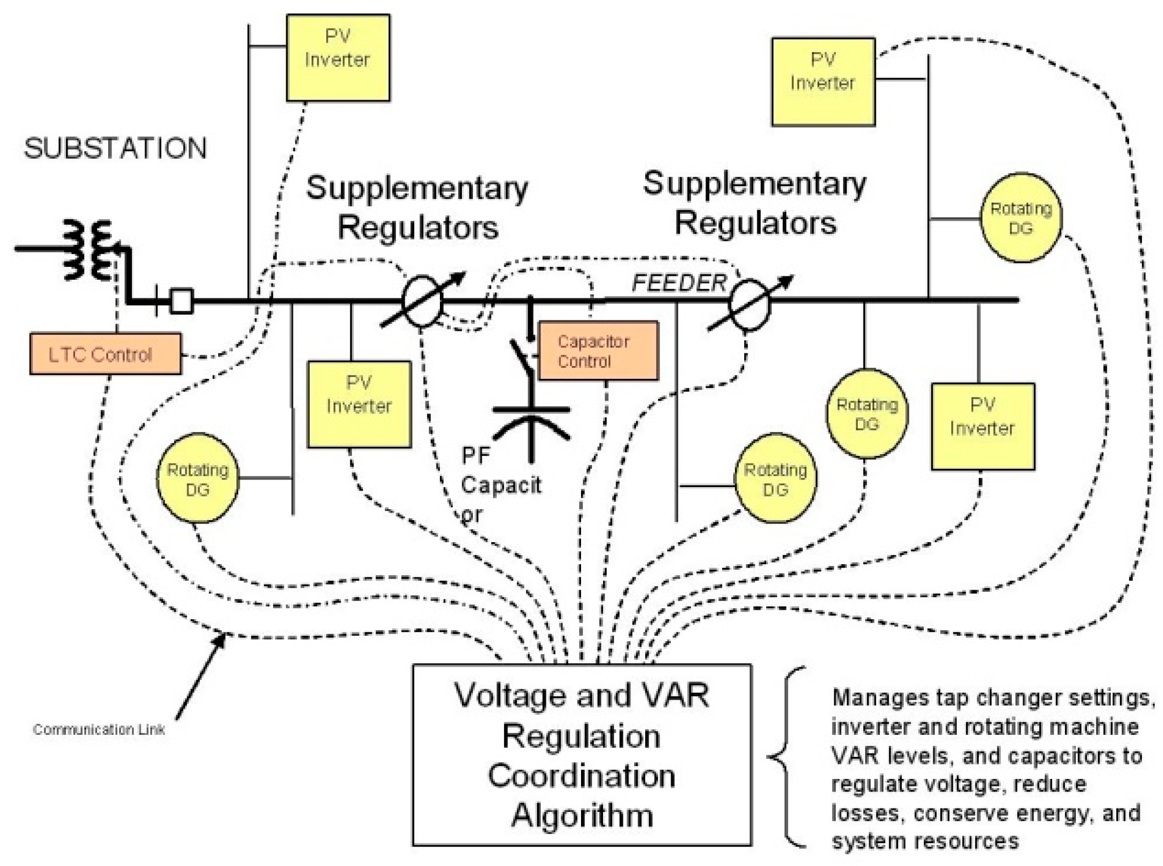
Volt-var optimization involves controlling voltage levels and reactive power as efficiently as possible to improve grid operation by lowering system losses, peak demand, energy consumption, or any combination. It collects real-time grid data using sensors, smart meters, and SCADA systems. Figure 1 displays a representation of the VVC devices used in a distribution system given in [15].

There is no coordination between the voltage control devices since they are typically controlled locally by local controllers, such as the switchable capacitors, voltage regulators, and controllable load tap changer transformer. The studied technique intends to offer coordination between the VRs and CAPs to maintain optimal VVC performance even on systems with rapidly changing operational conditions, such as the penetration of DGs into the systems.

VVO aims to reduce the power loss on a distribution circuit or the overall MW demand a substation meets. The controllers are the voltage regulation devices’ tap settings and the capacitor banks’ switching state. The combined optimization of voltage and VAR faces two fundamental challenges.

• Exact modeling of the distribution system’s behavior under any control scenario.
• A reliable and effective search technique for optimization to offer a discrete solution for the taps of voltage regulating devices and the status of the capacitor bank. A solid VVO solution strategy should be capable of managing large, real distribution networks that have any of the characteristics.

VVO is a non-linear combinatorial optimization problem that primarily has the following features:

• The tap position of regulating transformers and the switching status of capacitor banks are both integer variables.
• System demand or power loss are implicit functions of the controls, which are an implicit function of the decision variables (continuous, real numbers) for a nonlinear objective.
• In the multiphase system model, there are thousands of power flow equations with high-dimension nonlinear restrictions.
• Non-convex objective function and solution set.
• The number of control variables in the high-dimension search space.

It is challenging to create an effective search algorithm for situations involving mixed integer nonlinear, non-convex (MINLP-NC) systems. An effective algorithm produces a global optimal or extremely close-to-optimal result.

3. Volt-Var Control and Optimization Problem Formulation

An integrated approach is used to conceptualize the problem. Switchable capacitor banks, VRs, and smart inverter’s active and reactive power outputs are dependent on the PV performance due to solar irradiance and are incorporated into the power flow calculation to examine the implications of status changes of these regulating devices on distribution system operation. We suggest voltage regulation and power loss reduction with the control of these devices. According to ANSI standard C84.1, the objective of VVC is to maintain the node voltages on a feeder within the permissible limits under all loading scenarios [16]. LTC and VRs can commonly change the voltage by 10% in 16 stages [17]. Normally, only one phase of voltage is monitored, but the distribution station’s LTC action affects all three phases. VRs are also controlled similarly but are often configured to control the voltage on each phase separately and can be connected anywhere on the feeder. In the meantime, adding power loss minimization and keeping voltage fluctuation at a minimum level (and not increasing the operational movement of frequent tap changing and capacitor switching not to reduce the life expectancy of these devices) to the VVC problem, it becomes an optimization problem—VVO can be formulated as a control and optimization problem such as (1)–(3):

$$\min (f(x)=P_{loss}=P_{gen}-P_{load})$$

(1)

$$P_{gen}=P_{GRID}+{\displaystyle \sum _{i=1}^k{P}_{PVi}}$$

(2)

subject to

$$\begin{array}{c}{g}_i(x,u)=0\hspace{1em}\hspace{1em}i=1\dots n\hfill \\ h_k(x,u)\le 0\hspace{1em}\hspace{1em}i=1\dots k\hfill \\ V_i^{\min }\le V_i\le V_i^{\max }\hfill \\ 0.95\le V_i\le 1.05\hfill \\ 0\le u_{cap}\le 1\hfill \\ -16\le u_{tap}\le 16\hfill \\ I_{microgrid}^{\min }\le u_{Imicrogrid}\le I_{microgrid}^{\max }\hfill \\ 0\le I_{1,microgrid}\le 219.97\hfill \\ 0\le I_{2,microgrid}\le 65\hfill \\ 0\le I_{3,microgrid}\le 169.12\hfill \end{array}$$

(3)

Details for power-related and microgrid current injections to grid-related formulas are given in Appendix A, Equations (A1)–(A10).

This VVC problem needs to be fixed for each feeder at each control update interval (which could be 1 min, 5 min, or 1 h), and the updated device settings need to be sent to the local controllers. This is a nonlinear mixed-integer combinatorial programming issue since the control u in this scenario takes discrete variables but with the connection of microgrid continuous variables as well. This problem then becomes computationally difficult.

Binary numbers are used to describe the status of a switched CAP, and hence the search vector for capacitor u is provided below (4):

$$\begin{array}{l}{u}_{capi}=[0,1]\\ u{1}_{cap}=[u_{cap1},u_{cap2},u_{cap3},\dots ,u_{capl}]\\ combination1=2^l\end{array}$$

(4)

where

l is the total number of reactive power suppliers/CAP, i = 0, …, l.

Tap numbers for LTCs and VRs are provided as integer numbers and generally have 32 tap positions. Each tap step size in this instance is 0.00625 V in p.u. As a result, a VR produces a voltage boost or buck of 0.00625*tap V in p.u. as a real value for each position shift. For any voltage device that has a problem addressing 32 possible tap settings or discrete variables, there will be a significant combination of tap settings if there are several voltage devices on the system. For example, there are 1,048,576 potential combinations even with one three-phase LTC and three one-phase VR, where m becomes 4.

$$\begin{array}{c}-16\le tap\le 16\\ u_{LTC/VR}=\left[u_{LTC},u_{VR1},u_{VR2},\dots ,u_{VRm}\right]\end{array}$$

(5)

$$\begin{array}{l}{u}_{tapi}=[-16,-15,-14,\dots ,0,\dots ,14,15,16]\\ u{2}_{tap}=[u_{tap1},u_{tap2},u_{tap3},\dots ,u_{tapm}]\\ combination2={32}^m\end{array}$$

where

m is the total number of tap units (VRs, LTC), i = 0, …, m.

The control variables from the microgrid are the current sources—ISources, I₁, I₂, I₃

$$\begin{array}{l}u{3}_I=[I_{1,microgrid},I_{2,microgrid},I_{3,microgrid}]\\ combination3=3^n\end{array}$$

(6)

$$\begin{array}{l}TotalCombination=combination1\ast combination2\ast combination3\\ TotalCombination=2^2\ast {32}^4\ast 3^1=12,582,912\end{array}$$

(7)

The formula for integrated possible combinations is given (7), and the number of combinations becomes just for two capacitors, four tap devices, and one microgrid with three current sources, 12,582,912. It is evident that when the system size and the number of control devices rise, the number of power flow calculations will increase significantly. The problem size grows exponentially, at the power factor of the number of decision variables for combinatorial optimization problems. To reach the global optimum settings of the devices by deterministically using brute force to solve the problem is hence inefficient in terms of computation cost and time. To achieve the actual or nearly actual answer, some new computational techniques may need to be constructed as investigated in our earlier research [13,14], or by employing metaheuristic algorithms. Here, we used a metaheuristic algorithm as the HS algorithm to solve the optimization problem in this study. The reason for choosing the HS algorithm is that when musicians compose a harmony, they usually try various possible combinations of the music pitches (notes-district variable) stored in their memory. This search for perfect harmony is indeed analogous to the procedure of finding the optimal solutions to engineering problems. The HS method is inspired by the working principles of harmony improvisation and is best used for discrete decision problems (e.g., capacitor bank scheduling, tap number optimization). It handles discrete and continuous variables.

The decision variables or control variables, vector x, which holds all integer numbers for CAP positions and TAP positions and real numbers for Isource from the microgrid (or P_PV and Q_PV) for the overall problem are given as (8)

$$\begin{array}{l}x=[u_{cap},u_{LTC/VR},u_{\mathrm{I},microgrid}]\\ x=[u_{cap1},u_{cap2},u_{LTC},u_{VR1},u_{VR2},u_{VR3},u_{I1,microgrid},u_{I2,microgrid},u_{I3,microgrid}]\end{array}$$

(8)

4. Harmony Search Algorithm

Meta-heuristic algorithms are essential to the field of computational science to solve challenging problems. The harmony search (HS) method is a population-based and iterative metaheuristic algorithm that draws its inspiration from the musical search for the ideal condition of harmony [18,19]. When a music orchestra attempts to create the most harmonious melody, it simulates the process of improvising a musical harmony. Similar to how the fitness function value affects the decision variables’ quality, each musical instrument’s pitch dictates its aesthetic quality.

• If every pitch creates a pleasing harmony, each musician remembers the experience from their memory and is more likely to create a more pleasing harmony next time;
• A similar way in optimization is that a set of initial solutions is produced at random from decision variables that fall inside the range of possibilities;
• If the objective function values of these choice variables are sufficient to yield a promising result, then there is a greater chance that a successful solution will be produced the next time.

HS algorithm parameters are

• Harmony memory (HM) matrix, which holds the initial solution (population).
• Harmony memory size (HMS).
• Harmony memory consideration rate (HMCR): It is an improvisation control parameter. It shows the probability of choosing a value of an element in a candidate solution vector from the existing HM matrix to improvise a new harmony.
• Pitch adjustment rate (PAR): It is also an improvisation control parameter that enables the development of new elements at the adjacency of the element in its HM matrix it is tuning.
• Maximum number of improvisations (MaxImp), which is the iteration number.

The three major duties are utilizing harmony memory, altering pitch, and randomization.

To build a new harmony from memory, the probability of choosing a value from the HM matrix is E₁, pitch adjusting is E₂, and random assignment is E₃:

xnew(i): p(E1) = HMCR ∗ (1 − PAR)	(a note in memory)
xnew(i): p(E2) = HMCR ∗ PAR	(adjacent to the note in its memory)
xnew(i): p(E3) = 1 − HMCR	(randomly choose)

The HS method is a powerful algorithm for unpredicted and uncertain systems that can handle linear and nonlinear, continuous and discrete variable datasets with greater performance.

The following are the key steps of the HS algorithm:

• Step 1:

Initializing the algorithm parameters.

Initializing the optimization problem control variables, which are tap values coming from the transformer and voltage regulator ($u_{LTC/VR}$) and on/off position of switchable capacitor ($u_{cap}$) parameter search space with a random generation and integer adjustment.

• Step 2:

Initializing the HM matrix by using uniformly randomized selection among the optimization problem control variable search space based on their ranges.

Then, the objective function f(x) (fitness value) for each candidate solution vector is calculated.

The harmony memory matrix with initial candidate solutions, fitness vector, and the parameters of HS algorithm are given below:

$$HM=\left(\begin{array}{ccc}{x}_{11}& \dots & x_{1n}\\ ⋮& \ddots & ⋮\\ x_{HMS1}& \cdots & x_{HMSn}\end{array}\right)$$

(9a)

$$f(x)=\left(\begin{array}{l}f1\\ .\\ .\\ .\\ f_{HMS}\end{array}\right)$$

(9b)

The HS algorithm parameters are set as follows:

• HSparams.HMS = 9 to 90;
• HSparams.MaxImp = 1000 to 10,000;
• HSparams.HMCR = 0.9;
• HSparams.PAR = 0.3;
• HSparams.b = (xU-xL)/100.

• Step 3: Improvisation of new harmony.

A new solution will be created according to the Algorithm 1 given below.

This is the stage of improvising new harmony (pitch adjustment and randomization): Each element in a vector in the HM can be computed via three different conditions according to the HMCR, PAR, and randomization (1-HMCR).

Algorithm 1. Steps to generate a new candidate solution vector.

If r1 < HMCR then    Create a random solution candidate vector    else      Create a solution candidate vector such that      For each column in HM do        Randomly pick an element        Create a random numbers r2        If r2 < PAR then          With PAR probability perturb this element          This perturbation is +/− 1        end       end     end end

• Step 4: Calculate the fitness of the new candidate and then contrast it with the worst HM matrix response. If the potential solution is superior to the worst option retained in the HM, the worst solution will be substituted with it.
• Step 5: The algorithm will proceed to step 3 before repeating steps 3 and 4 until the stop conditions, such as the required precision level or the maximum number of iterations, are met (MaxImp).

5. Computational Complexity of the Search Algorithms

5.1. HS Algorithm

The computational complexity of the HS algorithm depends on the number of decision variables (control variables), population size, and the number of iterations. Here is a breakdown:

5.1.1. Notation

• N = Number of decision variables (control devices), problem dimension;
• HMS = Harmony Memory Size (population size);
• MaxImp = Number of iterations;
• f(x) = Fitness function evaluation time complexity (P_loss and power flow equations).

5.1.2. Complexity, Breakdown

Initialization

• A population of HMS harmonies (solutions) is randomly initialized;
• Each solution contains N decision variables;
• Complexity: O(HMS ∗ N).

Improvisation (Solution Generation)

• In each iteration, a new solution is generated by selecting values from Harmony Memory and applying randomization (pitch adjustment, random selection);
• This step scales linearly with N: O(N)

Fitness Evaluation

• The new solution is evaluated using an objective function.
• Complexity depends on how expensive f(x) is.
• In volt-var optimization, f(x) involves power flow calculations, which are O(f(x)) that is O(N²) to O(N³), depending on the method used (Newton–Raphson, Newton–Raphson with Jacobian, Gauss–Seidel, etc.).

Memory Update

• If the new solution is better, it replaces the worst solution in the Harmony Memory.
• This step requires a comparison with existing solutions.
• Complexity: O(HMS)

Total Complexity per Iteration Is O(N + f(x) + HMS)

For MaxImp iterations, the total complexity is O(MaxImp ∗ (N + f(x) + HMS))

5.1.3. Worst-Case Complexity in Volt-Var Optimization

In volt-var optimization, if power flow calculations are O(N²) or O(N³), then

O(MaxImp ∗ (N + N² + HMS)) or O(MaxImp ∗ (N + N³ + HMS)) (polynomial).

5.2. Brute Force

5.2.1. General Formula for Brute Force Complexity

In a brute force approach, all possible combinations of variables are tested. The total number of evaluations is D^N.

Thus, the total computational complexity is O(D^N ∗ f(x)),

where

• N = Number of control variables.
• D = Number of possible values per control variable.
• f(x) = Time complexity of evaluating a single solution (fitness function evaluation).

5.2.2. Complexity in Volt-Var Optimization

In volt-var optimization, decision variables include

• Capacitor bank switching (discrete).
• Transformer tap settings (discrete).
• Reactive power generation (continuous or discrete).
• Voltage control devices (discrete).
• Power flow equations (continuous).
• Current injections from DERs (continuous).

• For a system with N control devices, each has D possible settings and a power flow analysis that takes O(N²) or O(N³) time. The brute force complexity becomes
• O(D^N ∗ N²) or O(D^N ∗ N³) (exponential)

BF is impractical due to exponential growth with increasing control variable numbers. It becomes computationally infeasible. It is used in [13,14] developing a systematically reduced search strategy. HS is preferred for VVO in this research because it provides near-optimal solutions with less computational complexity.

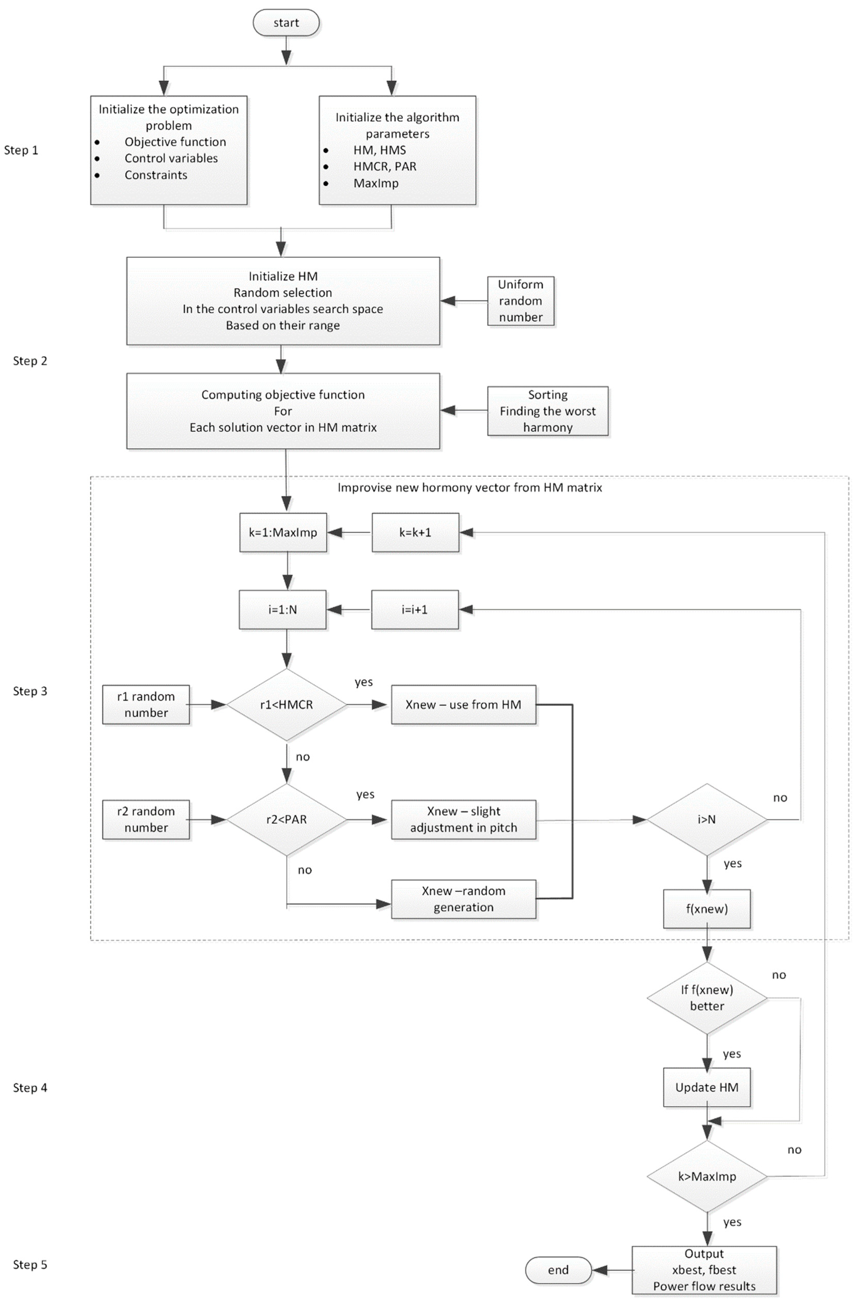
6. Coordinated Control of Volt-Var Optimization with HS Algorithm

Figure 2 provides a flow chart of the proposed problem solution procedures for coordination and optimization using the HS algorithm.

7. Test Systems

IEEE13 bus with a 16-node test circuit coupling with a microgrid is shown in Figure 3.

In the VVC/VVO problem, to optimize the flow of reactive power in electric power distribution systems and regulate voltage levels, the VVC part controls voltage and reactive power by using VRs and OLTCs for voltage and capacitor banks for reactive power, as well as DER integration for active/reactive power flows. The VVO part focuses on minimizing power/energy losses, maximizing efficiency, smoothing peak power demand, and maintaining voltage within regulatory limits.

Table 1. Control variables (voltage, reactive power, and active/reactive power devices).

Control Variables	Location (Bus No.)	Ranges
LTC	650.1.2.3–RG60.1.2.3	−16, −15, …, 15, 16
VR, reg1, (ph a)	670.1–671.1	−16, −15, …, 15, 16
VR, reg2, (ph b)	670.2–671.2	−16, −15, …, 15, 16
VR, reg3, (ph c)	670.3–671.3	−16, −15, …, 15, 16
CAP, cap1	675.1.2.3	600 kVar
CAP, cap2	611.3	100 kVar
ISource, I1, microgrid	675.1	0, …, 219.97 A
ISource, I2, microgrid	675.1	0, …, 65 A
ISource, I3, microgrid	675.1	0, …, 169.12 A

lists the control variables’ connection points shown in the OpenDSS notation and their ranges for the circuit.

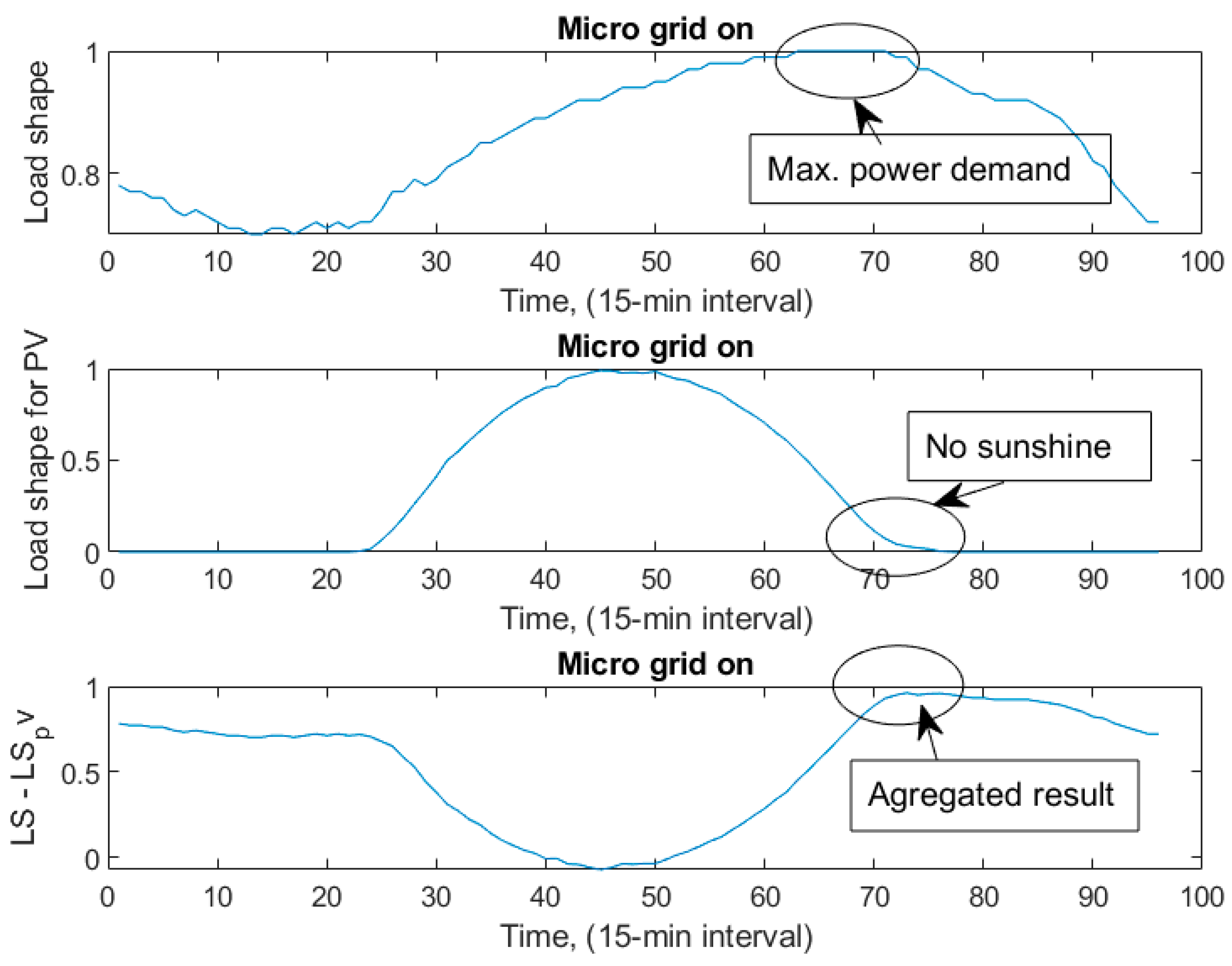
A typical daily load profile for the distribution system and a PV load profile with 15 min sampling are shown in Figure 4. The figure at the top is for the main grid, and the one at the middle is for the PV-based microgrid. The figure at the bottom is the aggregated form of both load shapes.

In Figure 4, a modified IEEE13node test circuit (.mod2) load shape (LS) is used for the main grid load. Load shape PV (LS_pv) is used for the microgrid. The resulting daily load shape or the net demand curve is determined by LS − LS_pv and looks like a duck curve [20].

For simulations of unbalanced power flow, the Matlab^TM environment and OpenDSS are used [21].

A microgrid example used here is taken from the OpenDSS package (the last modification date is 20 November 2019), the IEEE 13 bus test case. It is an example of simulating a microgrid using three current sources, ISource.

OpenDSS is open-source software that has COM interfacing capabilities, allowing the present control algorithms to be modified. The COM enables communication with OpenDSS solution output, circuit parameter modification, and OpenDSS command execution.

OpenDSS can be used to solve the power flow problem, and MATLAB can be used to write code for controlling or monitoring voltages and currents and operating the devices using the developed algorithms. All OpenDSS control blocks should be set to off mode to avoid conflict between two algorithms trying to control the same object [21].

The substation transformer’s low-voltage bus, which is where the microgrid connects electrically to the utility system, is known as the point of common coupling (PCC) for the system [22]. A block diagram of the PV System element model is provided in the OpenDSS manual [23].

To simulate Microgrid 3, separate, single-phase I sources are added, as shown in Figure 3. Each current source holds a different current level due to the unbalanced nature of the distribution system. One source followed the irradiance profile to simulate a PV. PV load shape is recorded as 1500 points in a day with a 1 min resolution. In the simulations, data are converted to 15 min intervals, the same as the main circuit grid load shape.

8. Cases

8.1. Case 1: On-Grid Operation of Microgrid, The Microgrid Is Connected to the Main Grid: Coordinated Control

Microgrid is on, and all control and coordination are performed on the Matlab platform.

In OpenDSS, for the power flow solution, daily load profiles for the grid and PV are disabled, and the control mode is set to off for regulators and capacitors. The Matlab platform is used for all management and coordination.

8.2. Case 2: On-Grid Operation of Microgrid, The Microgrid Is Connected to the Main Grid: Conventional Control

Microgrid is on, but conventionally locally controlled and not coordinated. It is called the base case.

Control mode is set to on for regulators and capacitors in OpenDSS. Load shapes for grid load and PV are still disabled here. Loads and current sources are updated according to each load shape for a day in Matlab.

8.3. Case 3: Off-Grid (Islanded) Operation of Microgrid. The Microgrid Is Separated from the Main Grid: Coordinated Control

The microgrid is off. All control and coordination are performed on the Matlab platform.

Load shapes for grid load and PV are disabled, and control mode is set to off for regulators and capacitors in OpenDSS. Matlab is used to handle each one.

8.4. Case 4: Off-Grid (Islanded) Operation of Microgrid. The Microgrid Is Separated from the Main Grid: Conventional Control

Microgrid is off but conventionally locally controlled and not coordinated. It is called the base case.

Control mode is set to on for regulators and capacitors in OpenDSS. Load shapes for grid load and PV are still disabled here. Loads and current sources are updated according to each load shape for a day in Matlab.

Details regarding each case simulation and comparison are presented in the next section.

9. Test Results

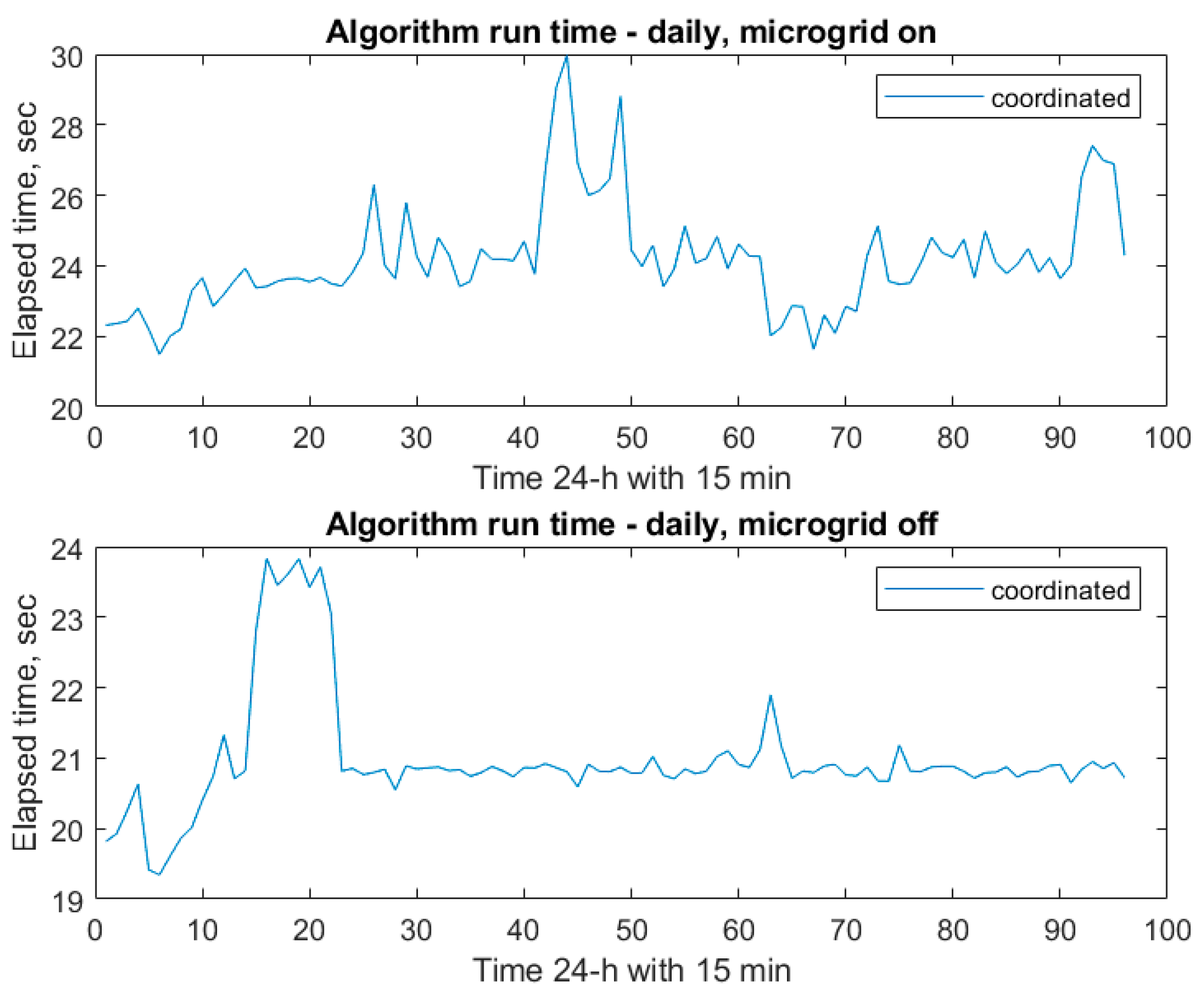
The HS algorithm is successfully applied on the MatlabR22b version. The running time for a day pattern is recorded as an example for both the microgrid’s on-grid and off-grid operations, as shown in Figure 5.

The PC specifications are as follows:

Intel Core i7-8550U CPU @ 1.80 GHz, 16 GB RAM, 64-bit operating system.

As seen from Figure 5, the elapsed time range was between 19 and 30 s. This work could be either used for planning or real-time applications due to its considerably fast running time.

The elapsed time varies more when the microgrid is on-grid than off-grid, even with coordinated control. The inverter operation of the PV circuit may cause these variations.

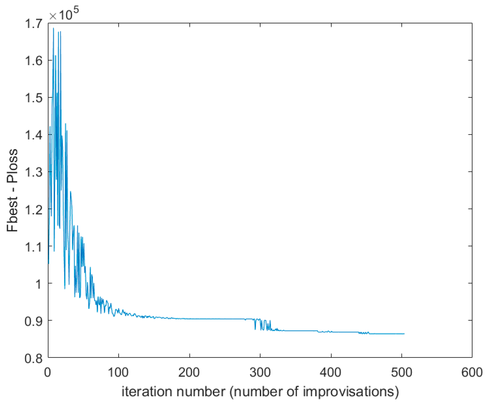
Figure 6 shows how the HS algorithm approaches the optimal solution in terms of active power loss minimization. The algorithm was tested on over 5000 iterations to check if it improves the objective. However, with each run, it stabilized at a maximum of 400 and did not improve. There is no need to increase the number of iterations and, hence, the simulation time.

Case 1: Microgrid is on-grid. All control and coordination are coded on the Matlab platform.

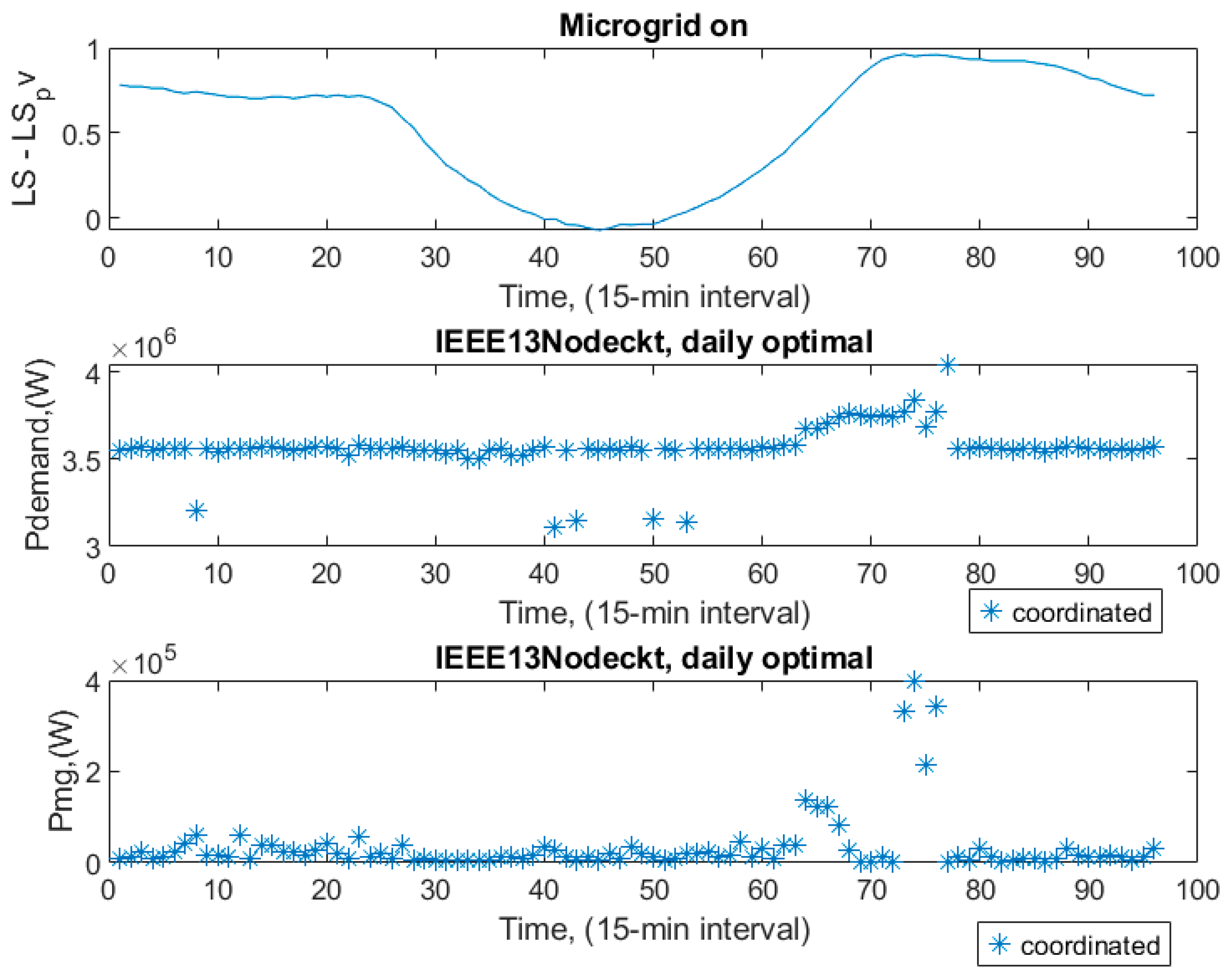
In Figure 4, according to the resulting daily load shape, the daily load demand from the main grid dropped to the lowest values when the microgrid fed the main grid around noon, which is the most productive time for PV cells. That decreased the overall active power loss, Ploss. The system works like two separate pieces. That means the current supplied by the microgrid is enough to feed the bottom part of the load on the main grid. Consequently, there is no need to draw any extra current from the grid. The proposed coordinated control strategy is verified with this result. The top part of the circuit is fed by the IEEE13node test circuit, and the bottom part of the circuit is fed just by the microgrid. The current flowing through the grid is decreased. That means the peak demand consumption, active power demand, and active power loss are all reduced.

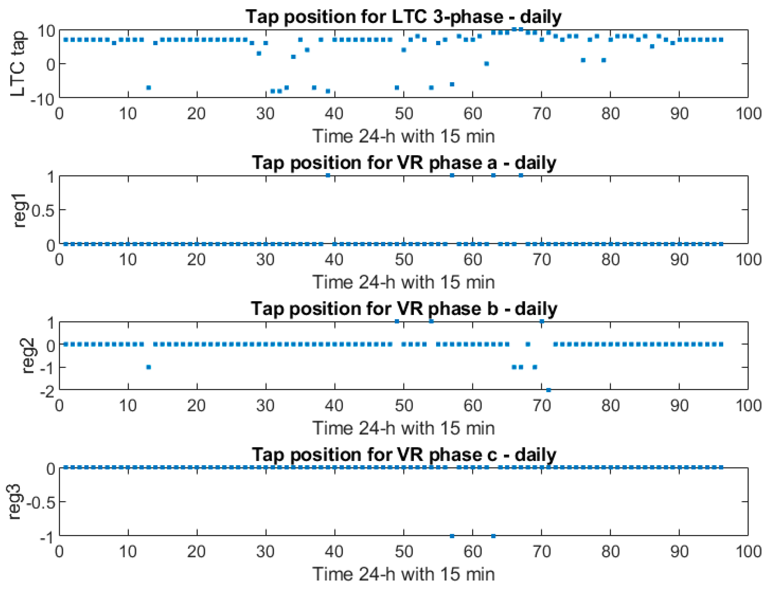
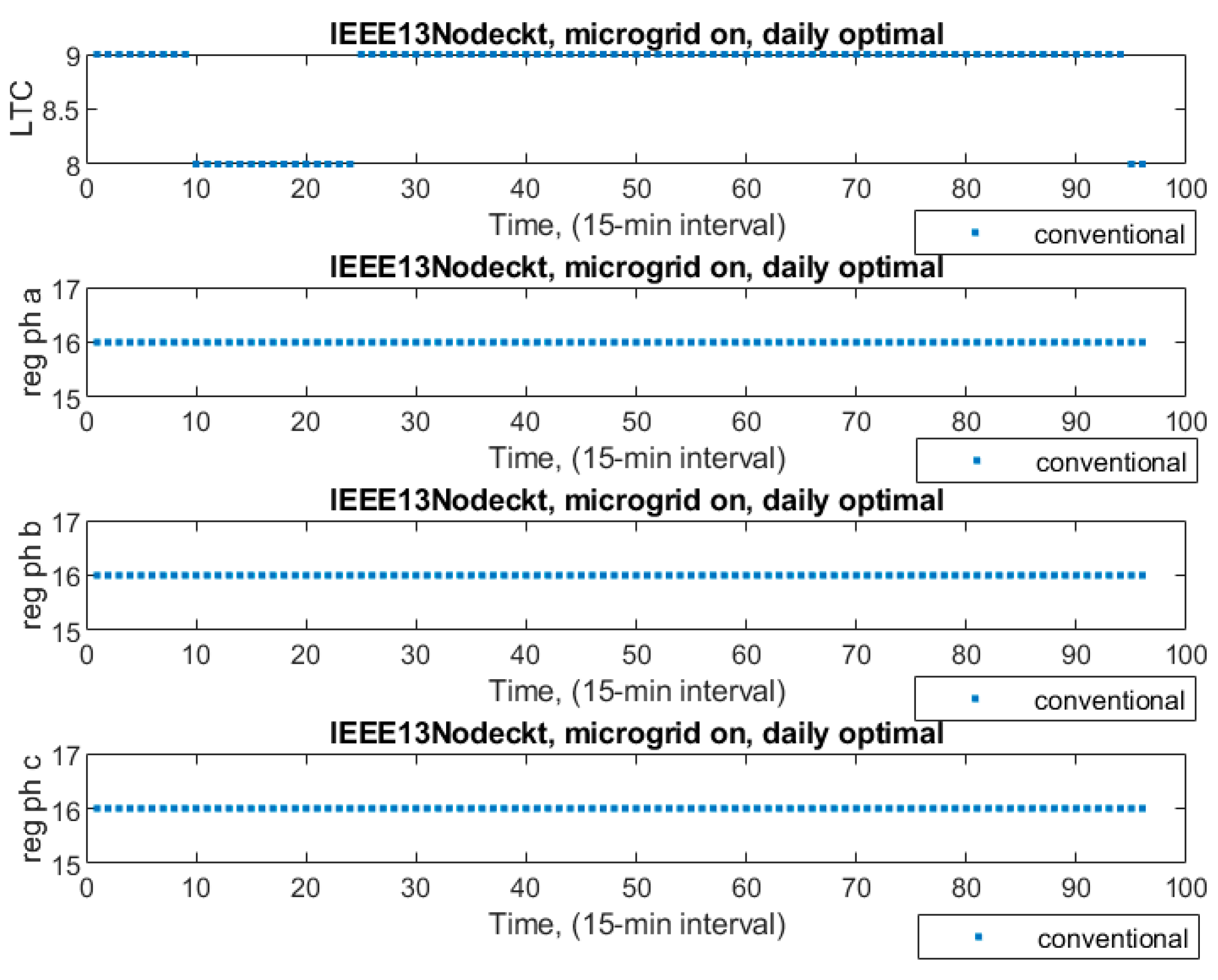
The time instance, a 15 min interval, of the day was between about 65 and 75 towards the evening, and evening time (4:15 PM through 7:15 PM) power demand increased from the main grid, as shown in Figure 4. Tap positions seemed to be changing, as seen in Figure 7. Depending on the unbalanced feeder load, some jumped to a higher level while others jumped to a lower level in order to feed the desired voltage level. During those time instances, reg1 moved between taps 1 and 0; reg2 moved between taps 1, 0, −1, and −2; and reg3 moved between taps 0 and −1.

Figure 7 shows that the LTC’s taps, which were three-phase and for the main grid, differed more than those of the other VRs. We observed the same discrepancies between single-phase units reg2 and reg3 and three-phase unit reg1. An unbalanced load section may also have been the cause of such.

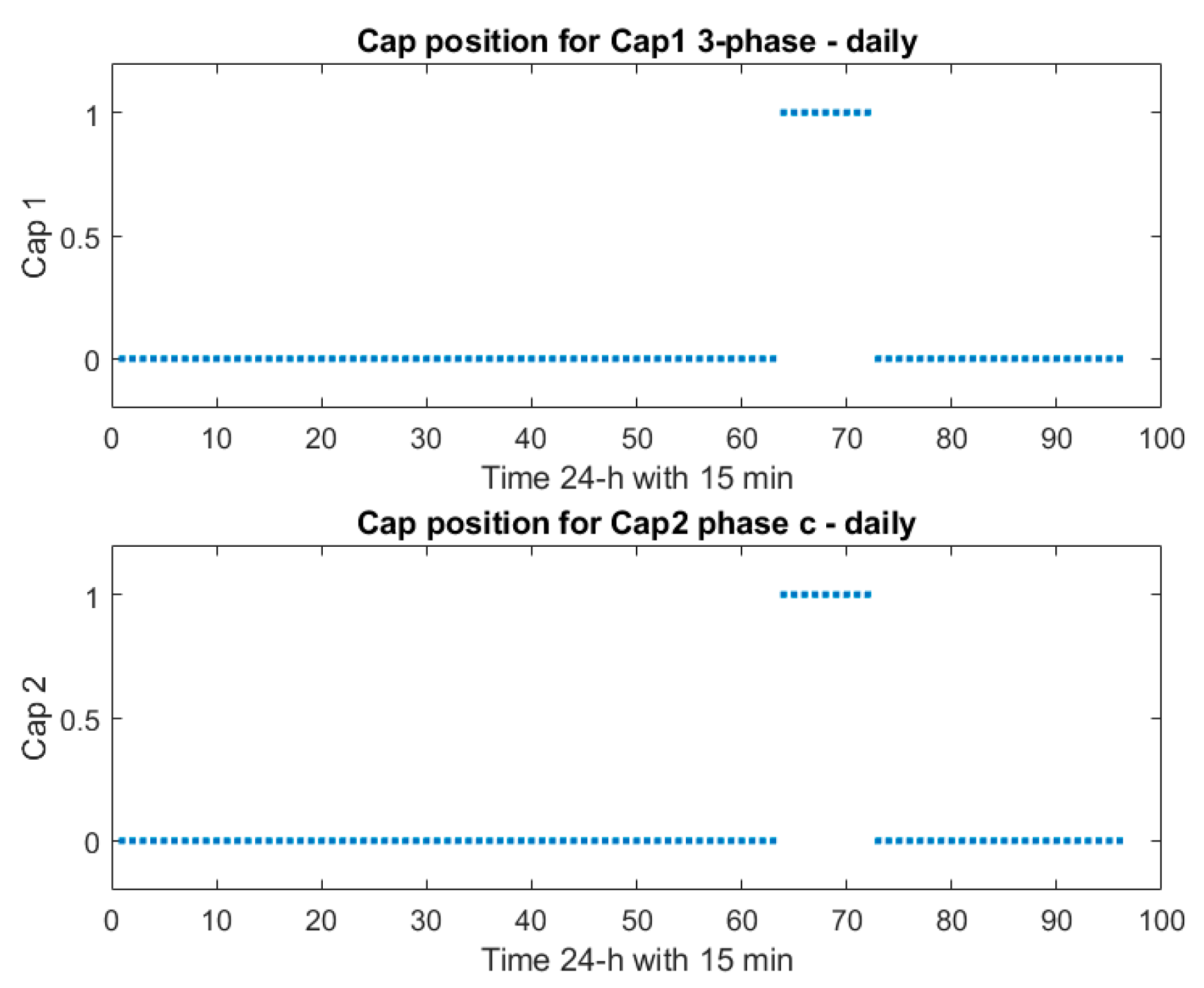
Both capacitors were turned on to provide the necessary reactive power where they were connected in the circuit for those rush time instances, as shown in Figure 8.

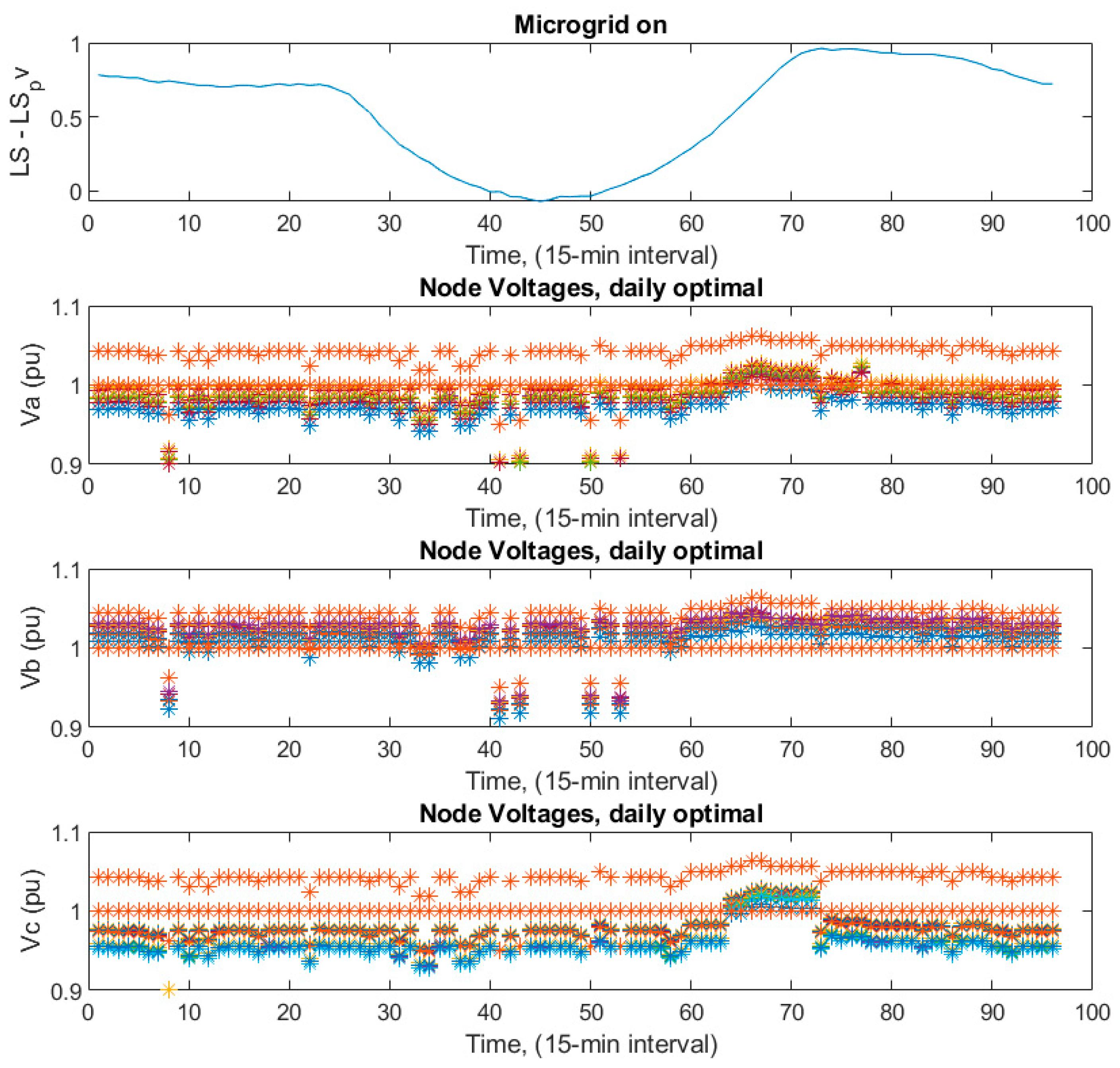
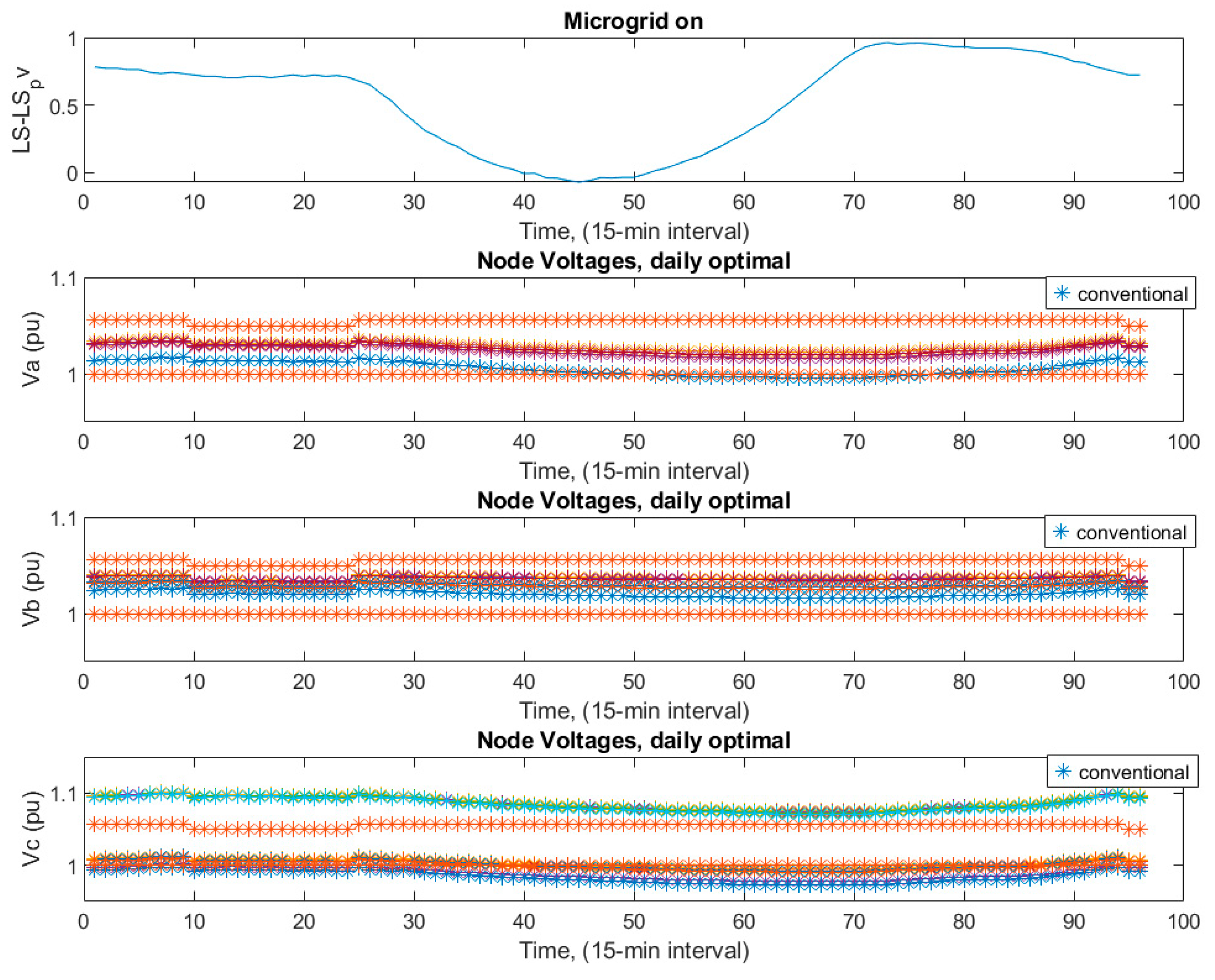
The node voltage levels started rising, as shown in Figure 9. The coordinated control ensured that the voltage levels were more stable together with the desired range 0.95 to 1.05 p.u. and fluctuations were minimized even though some of them for phase a and b went to 0.9 for a couple of time instances from time to time, mostly at around 1 p.u. all day long. As seen in Figure 9, the maximum voltage level for all phases belongs to bus number 650, which corresponds to the location where the LTC is connected in the test system in Figure 3. The situation is the same for the rest of the voltage figures.

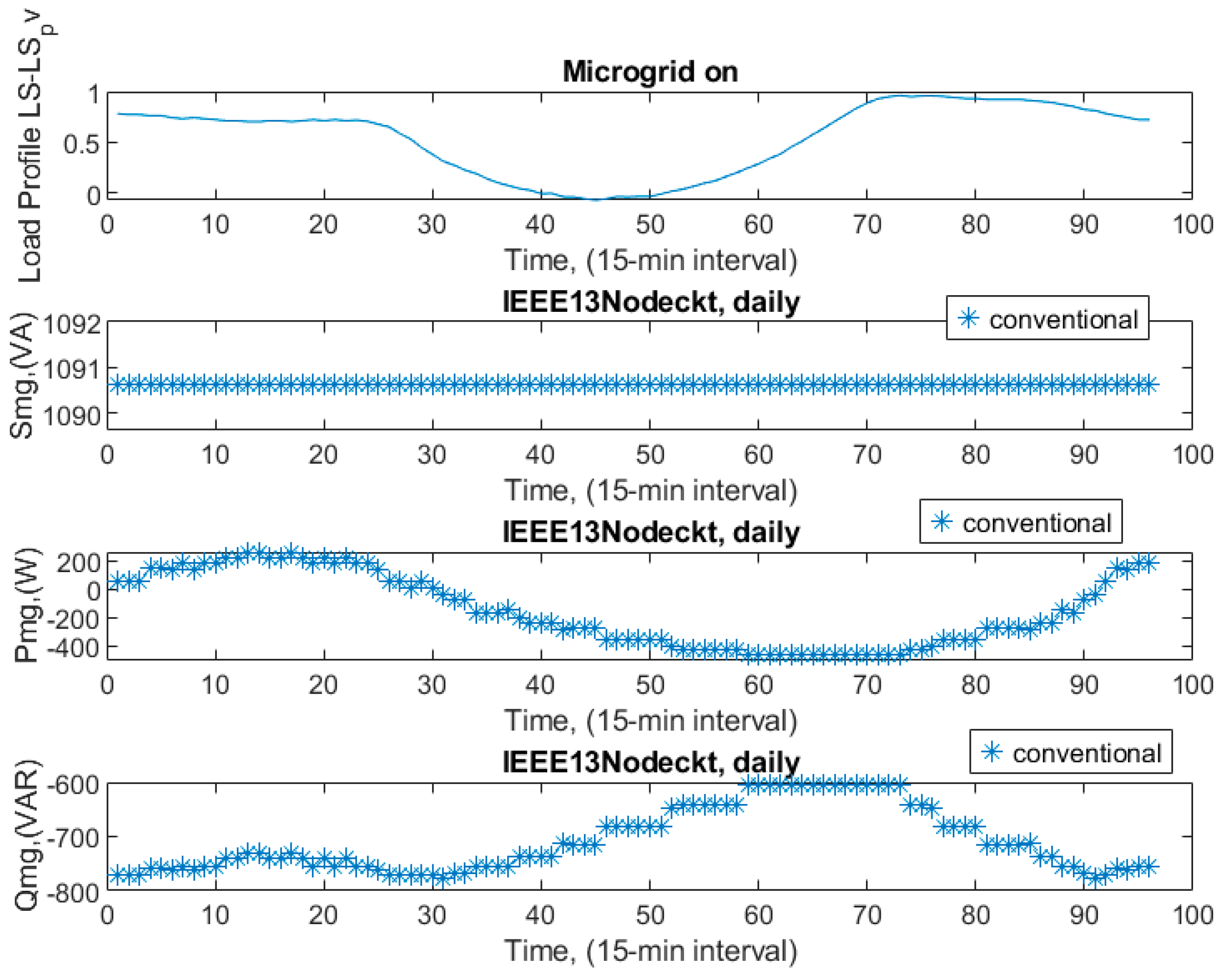
Between the time instances of the day, they were about 65 and 75 towards the evening, and evening time power demand was increasing. LS_pv was diminished. As Pdemand increased, in those time instances, state variables followed the pattern of the overall load shape, as seen in Figure 10 and Figure 11. In the majority of other time instances, we may conclude that the main grid’s active power demand and the microgrid’s active, reactive, and apparent powers were smooth, due to coordination.

Case 2: Microgrid is on but conventionally locally controlled and not coordinated. It is called the base case.

The control mode was set to on for regulators and capacitors in OpenDSS for the power flow solution. Load shapes for grid load and PV were still disabled here. Loads and current sources were updated according to each load shape for a day in the Matlab environment.

Figure 12 represents the locally controlled tap settings. In contrast to case 1, which was supervisory and centrally coordinated, where the LTC fluctuated between −10 and −10, it varied between taps 8 and 9 here. In this case, an operator set the value locally without taking the circuit’s overall information into account. For this reason, reg1, reg2, and reg3 did not change for that day and were all set to tap 16, which is required for the local needs.

These tap values for VRs were much higher than in case 1. They had the highest tap settings for all phases. Capacitors were switched on 1 at all times of the day. There were no variations, so the figure for cap1 and cap2 was not included. Due to the high tap setting, node voltage levels were almost all above 1 p.u, as shown in Figure 13. Even though voltage levels were in the range, it was not preferable to operate the system to have them above 1 p.u., very close to the upper limit. Consequently, total active power demand and losses were higher than the coordinated control, as shown in Figure 14.

As seen in Figure 14, the microgrid was on and connected to the main grid, but active power demand and loss did not follow the trend of the aggregated load profile. The reason for this was local control. The daily load profile of the main grid determined the active power demand and, in turn, the active power loss.

Apparent, active, and reactive power demand from the microgrid, daily pattern, and locally controlled are provided in Figure 15. Apparent power was constant for the day as expected from the local control. Active power followed the pattern of the load profile. When the active power flow started decreasing, the reactive power followed the opposite direction to keep the apparent power constant, which was expected, as indicated in Equation (A1).

Case 3: Microgrid is off. All control and coordination are coded on the Matlab platform with a coordinated control strategy.

Load shapes for grid load and PV were disabled, and control mode was set to off for regulators and capacitors in OpenDSS. Load shape for the main grid load and coordination were all handled in Matlab.

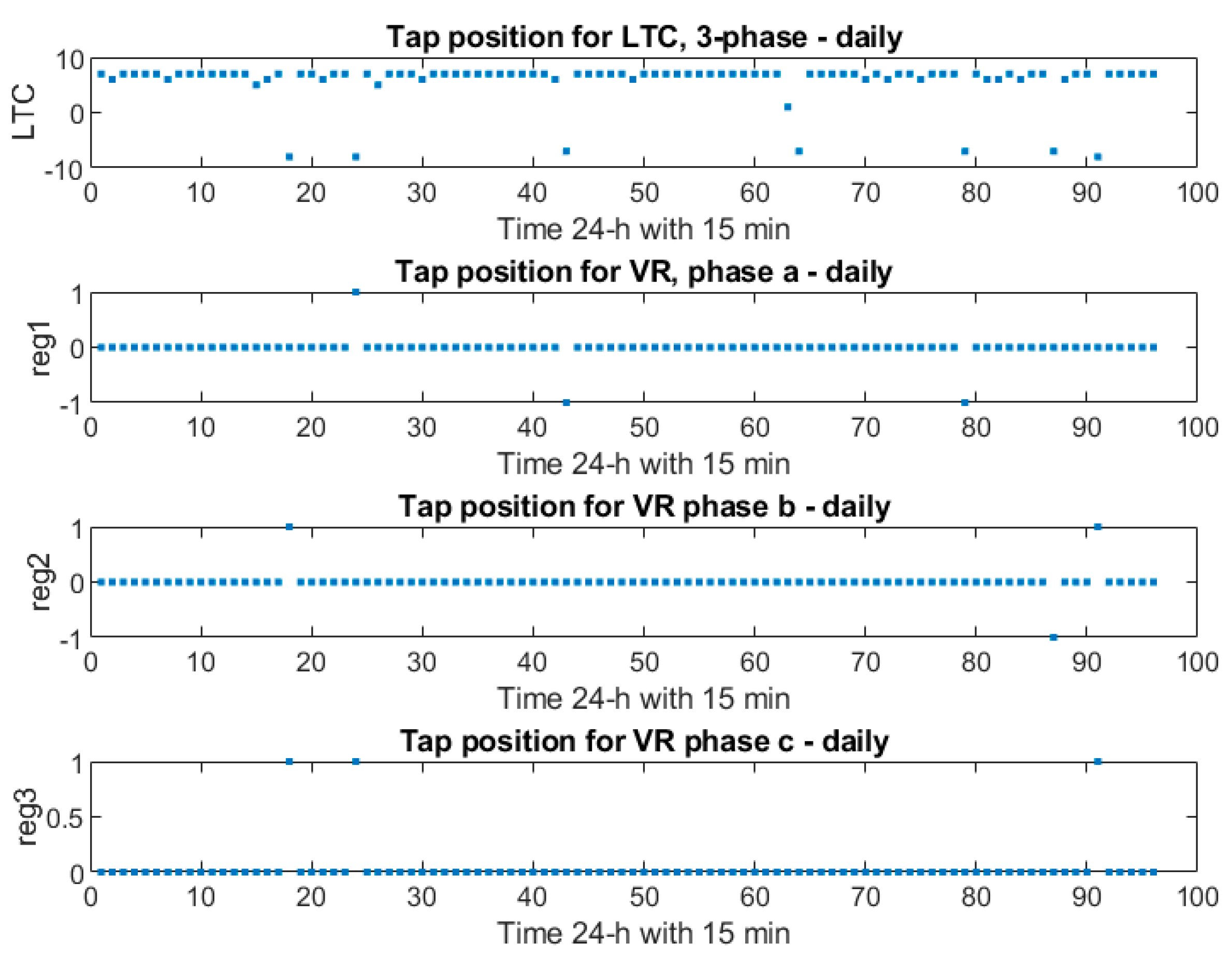
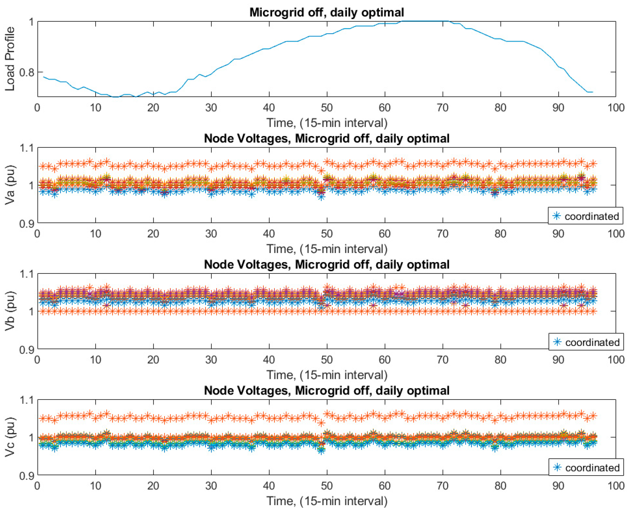
Tap settings are shown in Figure 16, and the node voltages in Figure 17 are comparable to case 1 in conjunction with microgrid node voltage levels that are nearly constant throughout the day. Due to coordination, fluctuation was also minimized with the heuristic optimization algorithm as an overall result.

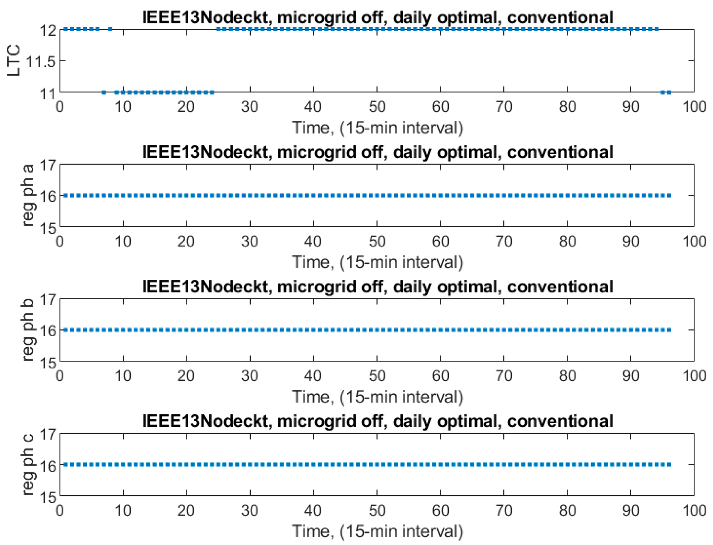
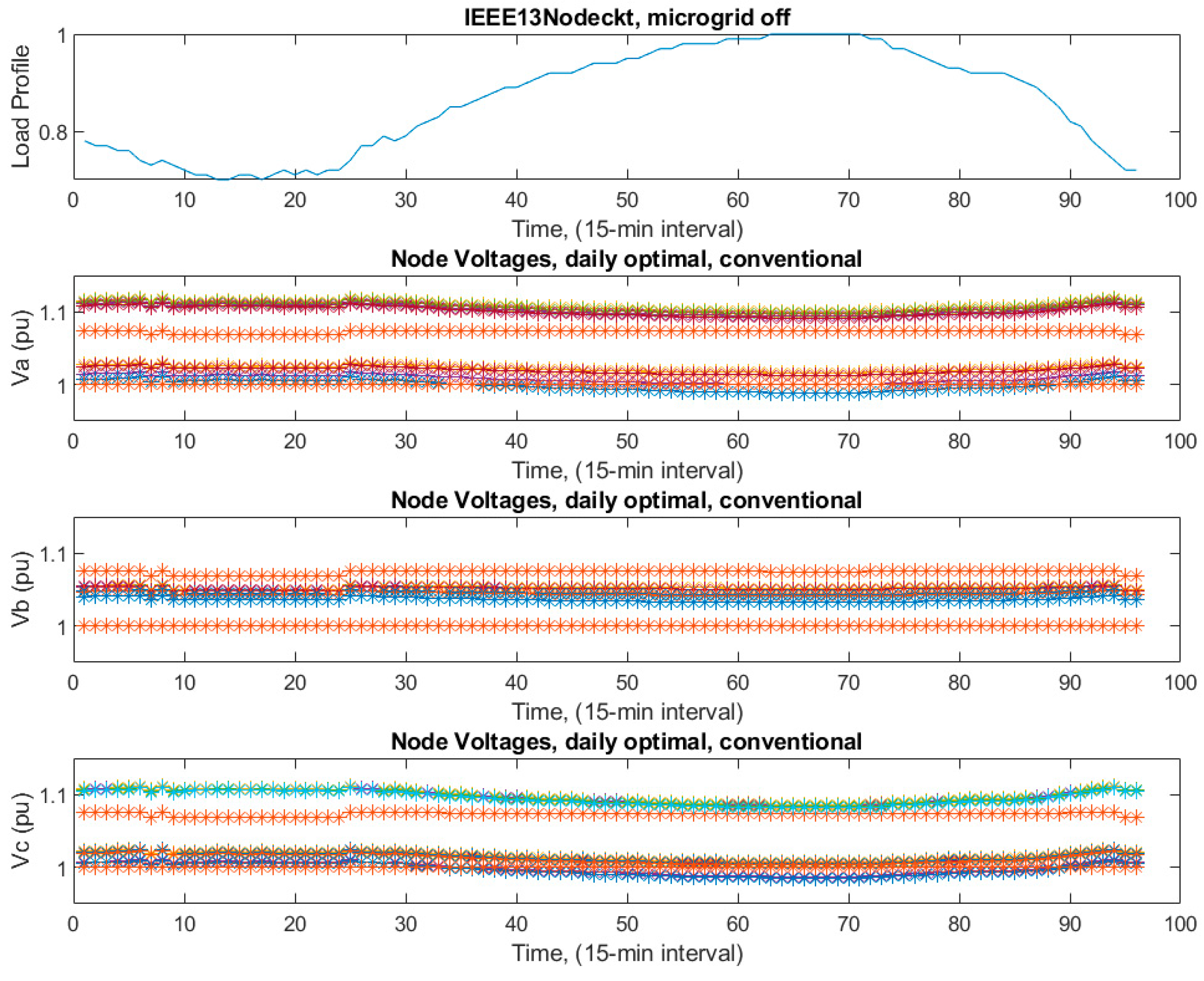
Case 4: Microgrid is off-grid, not coordinated, base-case conventionally controlled.

Only the daily load shape from the main grid is valid. As seen in Figure 18, tap settings were high as in case 2. Also, taps were the same for VRs for case 2 and case 4: both were conventionally controlled, even though in this case the microgrid is on here, and in that case, the microgrid is off. Again, capacitors are kept on 1 all day. Due to the high tap setting, node voltage levels were all above 1 p.u. and between 1 and 1.1 p.u., as seen in Figure 19.

Capacitor’s statuses were 1 for the whole day, at base case, conventional, and locally controlled with the microgrid off.

10. Comparison of the Cases

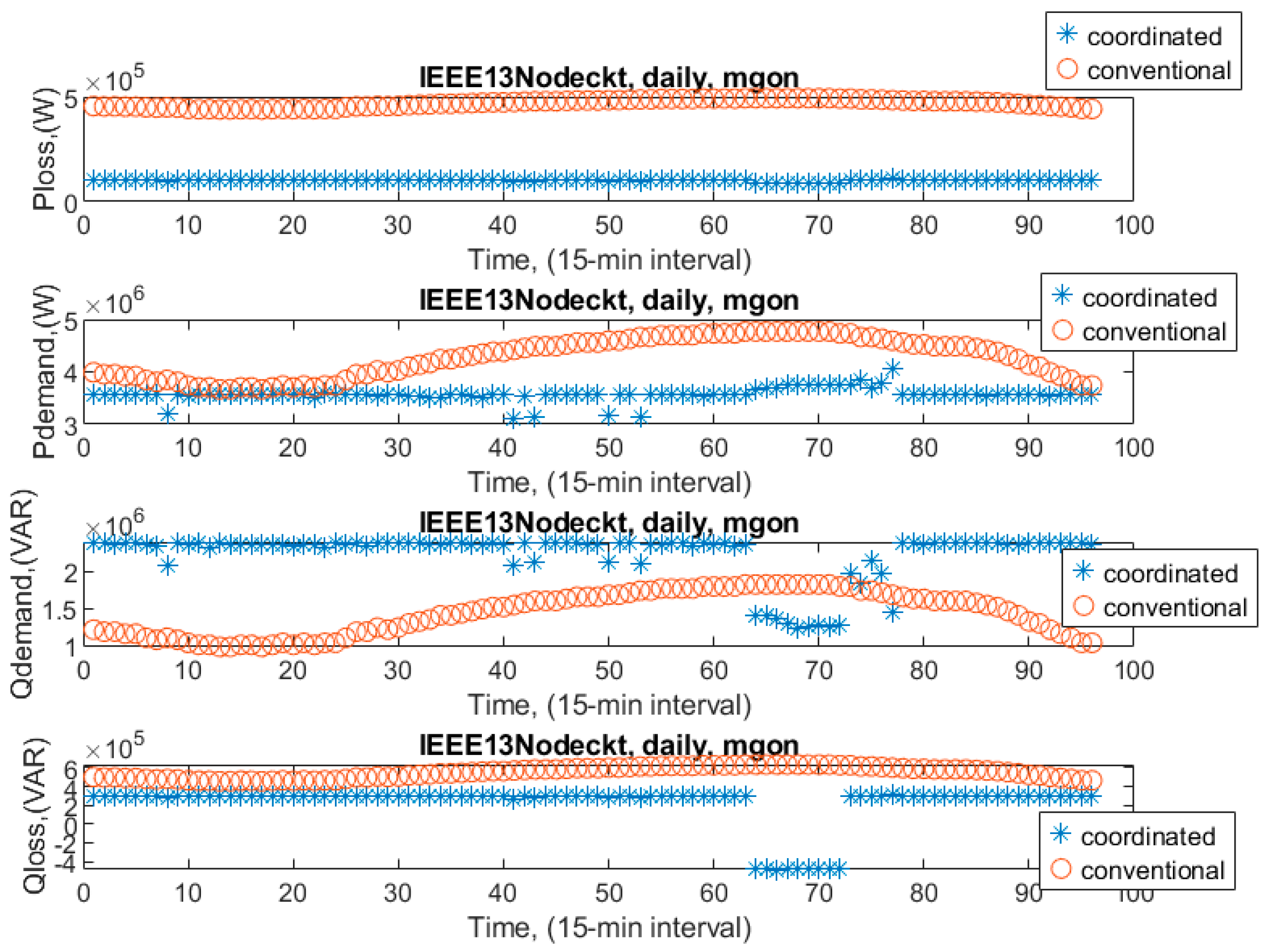
Comparison of base-conventionally controlled cases to the coordinated control when the microgrid was on:

Figure 20 presents the comparison results between the base case conventionally controlled and coordinated controlled. As seen from the figure and Table 1, active power loss decreased at the level of 78.04% just by coordination, which was a tremendous saving. Similarly, active power demand was reduced at the level of 16.54%, and reactive power changed daily with coordination. The microgrid provided extra electricity during peak demand hours when sun irradiation allowed for power production.

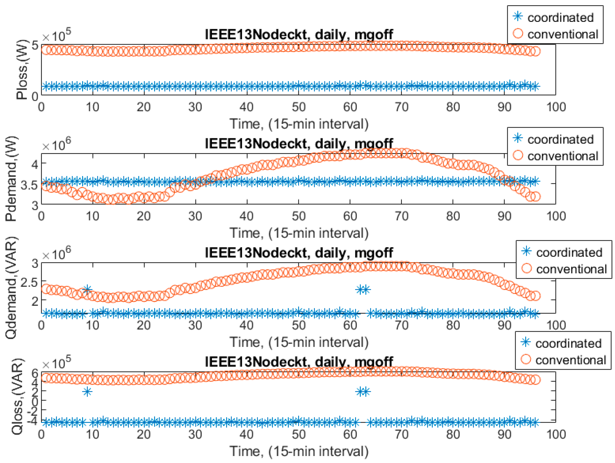
Comparison of base-conventionally controlled cases to coordinated control when the microgrid was off:

Figure 21 presents the comparison results between the base case conventionally controlled and coordinated controlled without the microgrid. As seen from the figure and

Table 2. Microgrid was on-grid, coordinated versus locally controlled, HS algorithm solution.

Daily Total	Conventional	Coordinated	Improvement (%)
Ploss (W)	45.0223 × 106	9.8877 × 106	78.04
Pdemand (W)	410.2777 × 106	342.4326 × 106	16.54
Qdemand (Var)	138.1709 × 106	213.9738 × 106	−54.8617
Sdemand (VA)	432.92 × 106	403.79 × 106	6.73

, active power loss was decreased at the level of 81.06% with coordination. The active power demand was reduced to around the level of 16.71%. This level was almost the same as the previous comparison, as shown in Table 1. The reactive power changed daily with coordination as well and was not close to the previous comparison, as shown in Table 1. Stable power consumption throughout the day was a significant outcome of this coordination. The peak active power demand was relieved well. That might have been due to good management of the reactive power with the coordination.

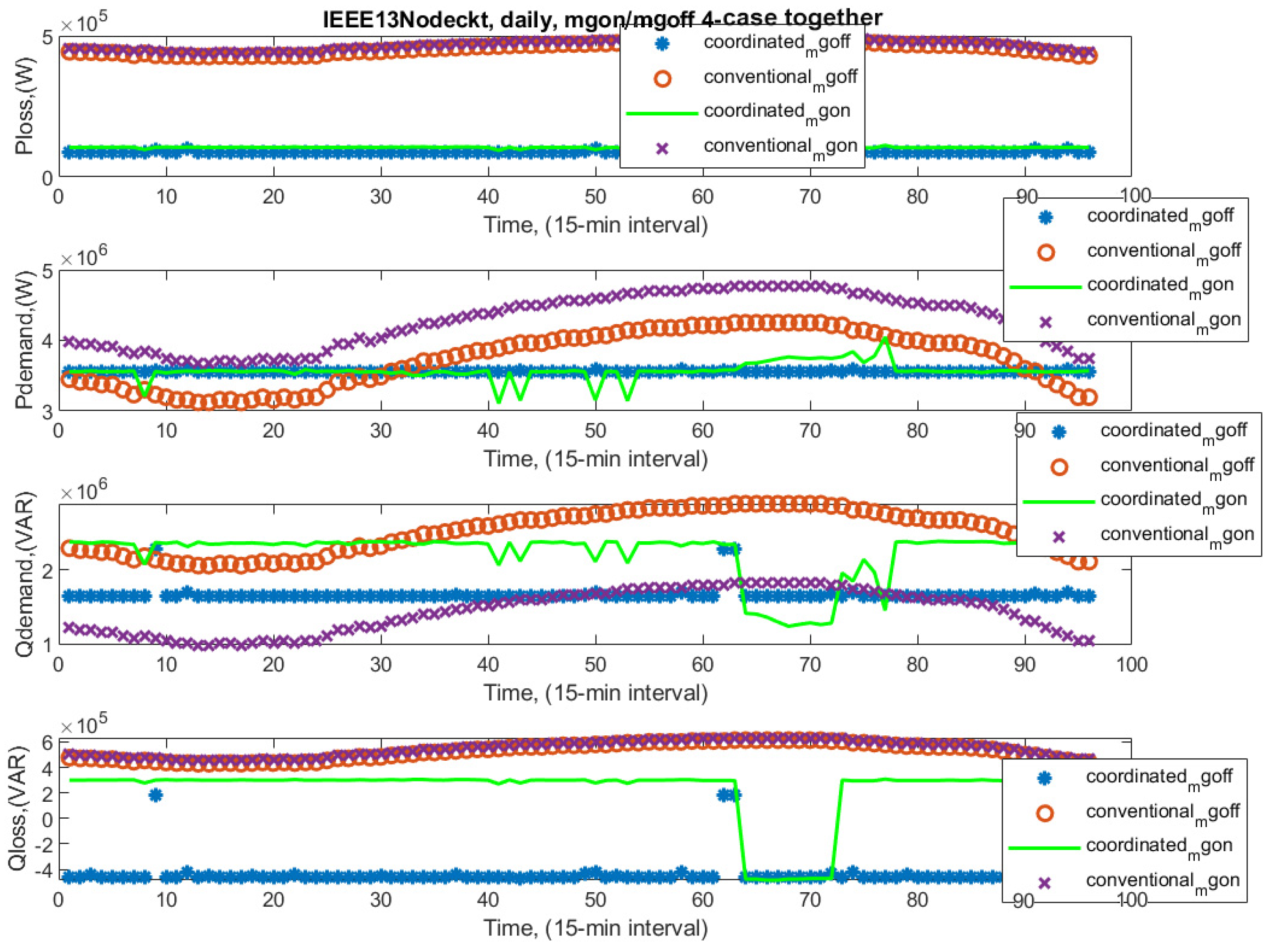
The comparison of all cases together is presented in Figure 22:

We can then conclude that coordination reduced quantities like Ploss, Pdemand, and Qloss. Effective power management was made possible through coordination. We still obtained highly effective power management even though there were minor swings while the microgrid was operating.

Table 2 shows how much gain was received after coordination while the microgrid was on for active power loss, active power demand, reactive power demand, and apparent power for the main grid. In terms of the daily cumulative saving ratio, we reached 78.04% minimization in active power loss and 16.54% minimization in active power demand. In our previous studies, power demand saving reached the level between 14% and 17.19% daily with coordination and CVR application [13]. Power loss saving reached the level between 75.79% and 84.43% daily with coordination [14], wherein the method used a brute force, deterministic approach with reduced search space as a systematic way to reach the global optimal solutions. Here, we used the heuristic optimization method. Even with the random characteristics of heuristic methods, we caught a good approximation optimal value at near-global in

Table 3. Microgrid was off-grid, coordinated versus locally controlled, HS algorithm solution.

Daily Total	Conventional	Coordinated	Improvement (%)
Ploss (W)	45.0223 × 106	8.5265 × 106	81.06
Pdemand (W)	410.2777 × 106	341.7011 × 106	16.71
Qdemand (Var)	138.1709 × 106	161.8527 × 106	−17.14
Sdemand (VA)	432.9200 × 106	378.1000 × 106	12.66

close to the deterministic results for global optimal values provided in

Table 4. No microgrid, coordinated versus locally controlled, deterministic solution [13].

Daily Total	Conventional	Coordinated	Improvement (%)
Ploss (W)	40.316 × 106	7.1335 × 106	82.31
Pdemand (W)	346.253 × 106	292.391 × 106	15.56

, without adding any effort to reduce the search space and using the decoupling future as used in the earlier study. On the other hand, when combined with microgrid integration, the heuristic approach shown in Table 1 saved around 1% less in active power consumption and 4% less in active power loss when compared to the previous study shown in Table 4.

Comparing apparent powers, 6.73% gain was received with microgrid integration while almost doubling 12.66% gain received without microgrid daily due to the coordinated control.

11. Discussion

This paper applied the HS optimization algorithm to the volt-var control and optimization problem to control and coordinate all associated devices, including LTC, voltage regulators, capacitor banks, and microgrid integration with PV systems on a distribution system. Four cases were simulated using an IEEE 13-node modified test circuit and a microgrid regarded as an IEEE 13 bus test circuit with PV represented by three current sources. The results were compared.

The first case was that the microgrid was on-grid with a planned coordinated control scheme. Less current passed over the entire main grid circuit due to the microgrid’s current supply. As a result, demand power and active power loss were drastically reduced. The heuristic algorithm’s randomness, which determines an ideal set point for the circuit decision variables at each time instant in a suitable manner, also prevented fluctuations in the nodes’ voltage levels.

The second case was that the microgrid was on-grid but no coordinated control scheme was designed. Volt-var-related devices were controlled locally with conventional control and no coordination. Capacitors were continuously on. Tap settings for VRs were at very high taps. This resulted in the node voltages being above 1pu and up to 1.1 pu.

The third case was when the microgrid was off-grid but a coordinated control system was applied. As a result of coordination, voltage levels between the nodes did not vary as much as in case 1, as expected due to the absence of PV-inverter operation.

The fourth case was that the microgrid was off-grid and not coordinated, and as the base case, it was conventionally controlled. The results were similar to case 2 due to the not coordinated related devices being controlled locally with conventional control.

As seen in Figure 9 and Figure 17, although both were coordinated controlled and voltages fell within the desired range, there were several abrupt variations and fluctuations during the day’s solar radiation period when the microgrid was operating on the grid. This could have been because of uncertainties in the PV system.

Both Figure 13 and Figure 19 demonstrate conventional control, with voltages falling within the upper bound of the permitted range. While voltages appeared to be smoother in both scenarios, voltage levels tended to dip slightly when power consumption was raised following daily patterns.

A comparison was made between the locally controlled and coordinated control cases when the microgrid was on-grid. Finally, coordinated control can yield a significant benefit. Furthermore, because of the microgrid integration and coordination scheme, peak demands were also met and handled smoothly.

12. Conclusions

The HS algorithm, a meta-heuristic-based optimization algorithm, was used in this study to handle the volt-var control and optimization problem under PV-based microgrid integration to the power distribution system. The main objective was to minimize active power loss while smoothing the peak power demands and keeping all node and phase voltages within the desired range to control and coordinate all voltage and reactive power-related devices for the most effective power management.

The coordinated control ensured that fluctuations were kept to a minimum throughout the day, with voltage levels remaining more stable within the intended range. Additionally, peak active power demands were fulfilled and managed efficiently due to the microgrid integration and coordination scheme.

Table 2 and Table 3 show a 3% difference in the active power loss reduction with and without microgrid integration; the microgrid-off scenario yielded a greater gain. As far as active power demand was concerned, the gains in both cases were nearly the same.

Table 3 and Table 4 show that, in the absence of microgrid integration, there was a 1% difference in the performance improvement between conventionally controlled and coordinated control for active power loss and active power demand when comparing the heuristic method HS algorithm with the previously studied deterministic method. It makes sense to consider the computational burden. The satisfying tradeoff was produced by the computational simplicity of the HS technique as compared to deterministic techniques.