Abnormal Load Variation Forecasting in Urban Cities Based on Sample Augmentation and TimesNet

Highlights:

What are the main findings?

• Abnormal load variations can be identified and characterized by the distribution of the residual component that is decomposed from the original city-level load series.
• TimesNet is an advanced and powerful deep learning model that can capture the complex load patterns during the abnormal load variation periods.

What are the implications of the main finding?

• It provides a generalized methodology of defining and quantifying the abnormal load variation events in urban cities to assist further analysis.
• It can improve the short-term load forecasting accuracy during abnormal load variation periods to enhance the power system operation stability and economy.

Abstract

With the evolving urbanization process in modern cities, the tertiary industry load and residential load start to take up a major proportion of the total urban power load. These loads are more dependent on stochastic factors such as human behaviors and weather events, demonstrating frequent abnormal variations that deviate from the normal pattern and causing consequent large forecasting errors. In this paper, a hybrid forecasting framework is proposed focusing on improving the forecasting accuracy of the urban power load during abnormal load variation periods. First, a quantitative method is proposed to define and characterize the abnormal load variations based on the residual component decomposed from the original load series. Second, a sample augmentation method is established based on Generative Adversarial Nets to boost the limited abnormal samples to a larger quantity to assist the forecasting model’s training. Last, an advanced forecasting model, TimesNet, is introduced to capture the complex and nonlinear load patterns during abnormal load variation periods. Simulation results based on the actual load data of Chongqing, China demonstrate the effectiveness of the proposed method.

1. Introduction

1.1. Background and Motivation

Short-term load forecasting is one of the critical preconditions for power system operation, and has been extensively studied in the last few decades. With the evolving urbanization process and industrial structure transformation, the tertiary industry load and residential load start to take up a major portion of the total urban power load. For example, according to the data released by the Shanghai government in 2024, the air conditioning load in Shanghai accounted for up to 50% of the total load in summer and 43% in winter. In such cases, the urban power load becomes more dependent on resident activities and weather conditions, which are stochastic in nature and make the urban power load fluctuate more. On the other hand, extreme weather events, such as heat waves and storms, have been occurring more frequently in recent years due to global climate change. Figure 1 shows the temperature profile and the aggregated load profile of over 1000 residential users in Austin, Texas in August 2017 [1,2] as an example. It can be seen that the load profile demonstrates unusual patterns during the two extreme weather periods. All the above facts lead to more frequent abnormal variations in the urban power load, causing large forecasting errors. Therefore, capturing these abnormal load variations (also called turning points in some studies) has become the focus of both the academic and industrial communities to further improve urban power load forecasting accuracy.

1.2. Literature Review

Studies that are relevant to the topic of abnormal load variation forecasting can be summarized into the following three threads:

The first thread focuses on the feature engineering process of the forecasting problem. In particular, weather features such as temperature and humidity have been extensively studied because weather conditions are highly correlated with the power load. Fay et al. [3] analyze the influence of weather forecasting errors on the load forecasting performances. In [4], the Heat Index is introduced by Chu et al. as a key input parameter for the load forecasting model. The Heat Index combines temperature and humidity to determine the apparent temperature, which is considered highly correlated with air conditioning loads and therefore can benefit the load forecasting model. Yu et al. [5] establish a two-level Intelligent Feature Engineering (IFE) framework to assist the short-term load forecasting model. Weather features are processed in the first-level IFE to reflect the load-weather dependency. Wang et al. [6] focus on the challenging forecasting problem of individual residential load. Meteorological variables are analyzed and introduced to the Long Short-Term Memory model to achieve forecasting. Instead of focusing on the common load–temperature dependence, Xie et al. in [7] study the impact of humidity on the power load and find that relative humidity is another important driving factor for power load, especially in warm months. A systematic approach is proposed to identify a group of humidity-based variables, based on which the load forecasting accuracy can be improved on different forecasting horizons. In [8], Hong et al. study the weather station selection problem to assign different number of weather stations to each forecasting zone automatically. The proposed framework can simultaneously determine the optimal number and the best choices by ranking and combining the candidate weather stations. Mansouri et al. in [9] propose a load forecasting model based on dynamic mode decomposition with control. Perceptible temperature is considered the most important external variable, reflecting a hybrid effect of temperature and humidity on humans. In [10], three temperature scenario generation methods are compared by Xie et al. in probabilistic load forecasting based on the quantile score. General guidelines for selecting scenario generation methods are proposed accordingly. However, despite the influence of weather factors on the load forecasting problem having been widely studied, abnormal load variations still lack a generalized and quantitative definition, which is considered another important aspect during the feature engineering process. Providing such a definition method can help identify abnormal load variation events and benefit the downstream forecasting model.

The second thread focuses on improving the load forecasting models to better capture the load patterns and load–weather dependency. In [11], Dehalwar et al. compare the accuracy of an Artificial Neural Network (ANN) and Bagged Regression Tree in urban power load forecasting. Weather forecasts are incorporated as the model inputs and are identified as important features to the forecasting accuracy. In [12], Lu et al. decompose the load profiles into base component and weather-sensitive component to conduct the forecasting separately. Meteorological data are used to train a Support Vector Regression model to forecast the weather-sensitive component. Following similar decomposition–aggregation methodology, Xu et al. in [13] propose a probabilistic forecasting model for building load forecasting. Weather features like dry-bulb temperature and relative humidity are included in the normal load forecasting model. Several forecasting models in the peak load forecasting of institutional buildings are compared by Kim et al. in [14]. Weather features are proven to be important external features to improve the forecasting performance. Considering the different load patterns between weekdays and weekends, Li et al. propose a semi-parametric load forecasting model in [15] focusing on weekend load forecasting. The coupling relation between meteorological factors and the load is considered, including the temperature accumulation effect. In [16], a systematic load forecasting approach is proposed by Pinheiro et al. covering from system level to low-voltage level. Numerical weather predictions, especially temperature, are used as explanatory variables. Simulation results based on 100,000 secondary substations in Portugal demonstrate the proposed method can improve the forecasting accuracy while maintaining good applicability, interpretability, and reproducibility. Guo et al. extend the power system load forecasting to an integrated energy system including cooling, heating, and electrical loads, as demonstrated by [17]. An attention layer is introduced to extract correlations among diverse loads, and an attentive quantile regression temporal convolutional network is proposed to achieve probabilistic forecasting. Weather variables such as temperature, humidity, and wind speed are incorporated as important model inputs. A theory-guided deep learning load forecasting model is proposed by Chen et al. in [18] that combines domain knowledge and machine learning. The machine learning model takes the weather forecasts as part of the model inputs and is robust to the weather forecasting errors by adding synthetic disturbances during the training process. In [19], Li et al. propose a two-stage electrical load forecasting method based on the fast-developing Internet of Things (IoT) system. Sensitivity analysis is conducted to identify the factor importance to the power load, among which temperature is recognized as a key factor. Note that although numerous efforts have been made to improve the forecasting model, the sample scarcity issue of the abnormal load variation forecasting problem has not been fully addressed. Because the abnormal load variations usually occur infrequently, the available data samples are much less than normal load samples, making it difficult to train complex forecasting models. It is necessary to propose sample augmentation methods to boost the limited abnormal load variation samples to a larger quantity, so that the numerous forecasting models can be well trained.

The third thread focuses on studying and characterizing extreme weather events, which usually occur in rare circumstances but lead to drastic load variations. Deng et al. [20] first establish an extreme weather identification model considering load, weather, and time factors to determine the occurrence range of upcoming peak load. Then, the Extreme Gradient Boosting (XGBoost) algorithm with Bagging strategy is proposed to forecast the short-term power load. Focusing on wildfire as the extreme event, Yang et al. [21] develop a wildfire resilient load forecasting model to enhance the load forecasting accuracy during wildfire season. The Fire Weather Index is used as the major exogenous factor to assist the deep learning-based forecasting model. 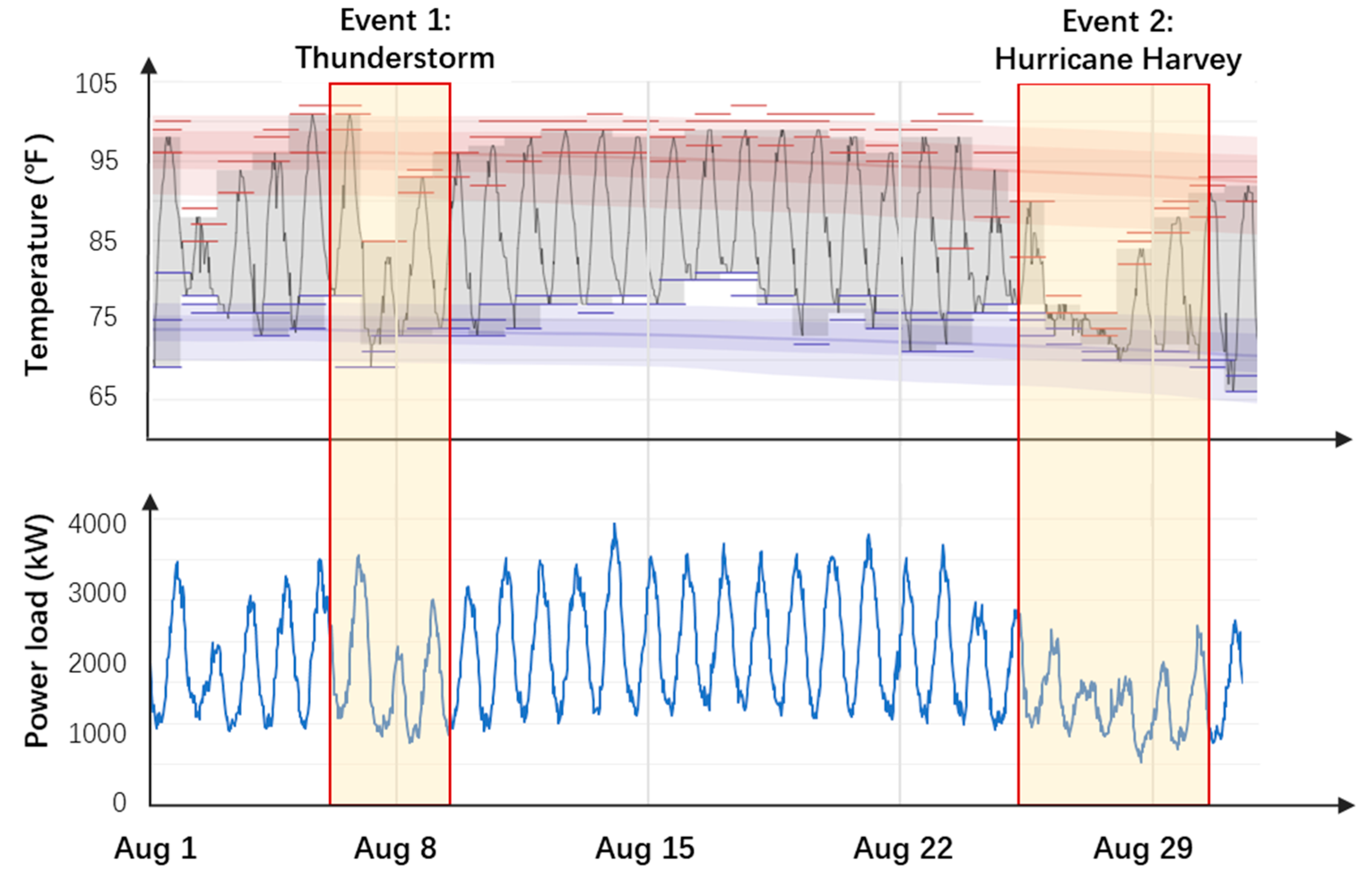In [22], Zhang et al. focus on the impact of hurricanes on the cascading failures of the EV charging networks. A probabilistic graphical model based on a Bayesian Network is proposed to model the correlations among different nodes, and an AC-based Cascading Failure model is implemented to simulate the power system cascading failure process. Shield et al. examine the disruptions of various types of extreme weather events, such as thunderstorms, winter storms, and tropical storms, to the electrical power grid [23]. Multiple indexes are established to quantify the impact, which provides valuable information for government and utility company decision-making. Considering the increasing penetration of solar and wind power in power systems, Watson et al. [24] study the power grid resilience with high renewable energy penetration under hurricane attack. Simulation results demonstrate that the generation capacity loss and the system restoration cost increase significantly for a power grid with high renewable penetration. Taking Hurricane Maria as an example, Kwasinski et al. [25] study the systematic impact of hurricane on the Puerto Rico power grid, including generation, transmission, and distribution. Results demonstrate that the resilience of the Puerto Rico power grid is weaker than the U.S. power grid under hurricane attack, requiring further investment and technological development. In [26], Fatima et al. provide an extensive review of power system outage prediction methods during hurricanes. Conclusions include that using a single machine learning model may lead to significant forecasting bias, which can be improved by implementing an ensemble learning strategy. It is also revealed that factors such as data quality, algorithm complexity, and model interpretability would be the focus in future research. However, as these studies mainly focus on the impact of extreme weather events on power system resiliency and economic loss analysis, their influence on the load forecasting problem has not been sufficiently discussed.

1.3. Research Gap

Based on the literature review in the above Section 1.2, three major research gaps can be identified on the topic of abnormal load variation forecasting, summarized as follows:

First, during the feature engineering process, existing studies (Refs. [3,4,5,6,7,8,9,10]) mainly focus on analyzing and quantifying the load–weather dependencies. There still lacks a generalized and quantitative definition for abnormal load variations, which could be another important feature of benefit to load forecasting models.

Second, when developing a forecasting model, existing studies (Refs. [11,12,13,14,15,16,17,18,19]) mainly focus on designing delicate model structures to better capture load variation patterns. However, as abnormal load variations usually occur infrequently, the limited number of datum samples may not be sufficient to train the increasingly complex forecasting models. It is necessary to introduce sample augmentation methods to boost the limited abnormal load variation samples to a larger quantity to enhance the forecasting model training.

Third, from the perspective of extreme weather events such as hurricanes, existing studies (Refs. [20,21,22,23,24,25,26]) mainly focus on their impact on power system resilience and economic loss analyses, while their influence on the load forecasting problem is less studied. It is important to discuss the load forecasting problem under such extreme weather conditions since they will significantly change the load pattern.

1.4. Contribution

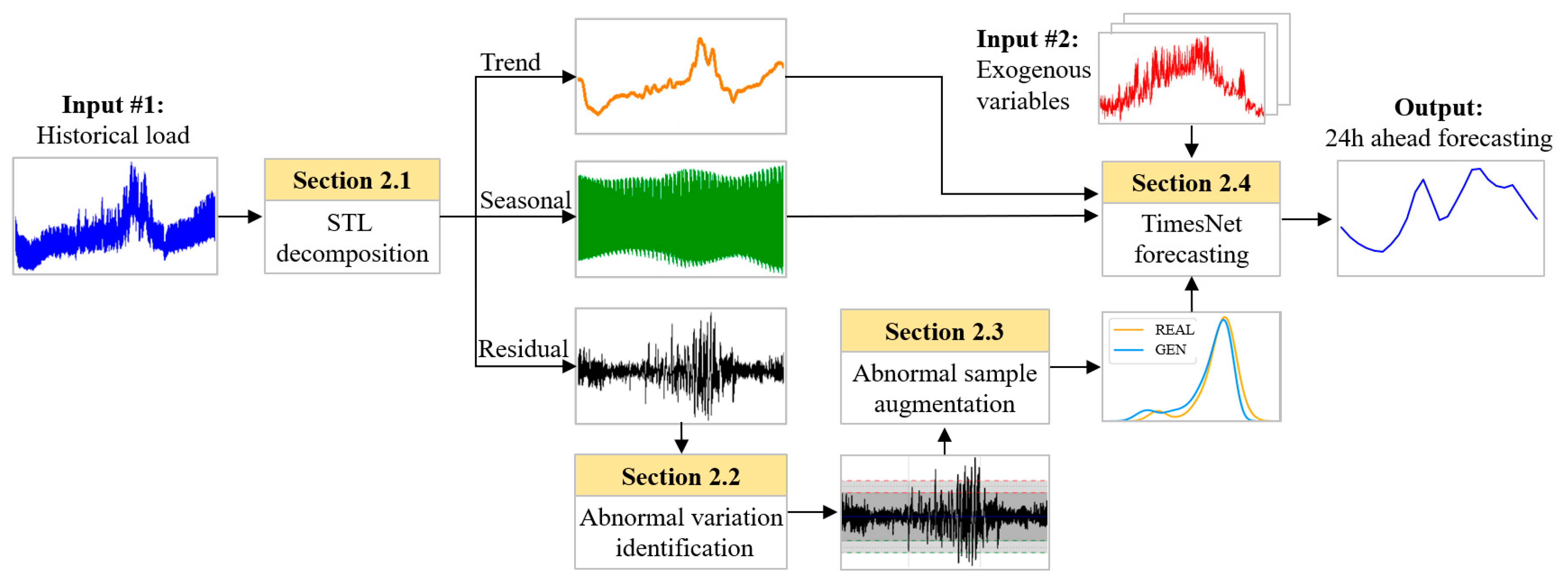
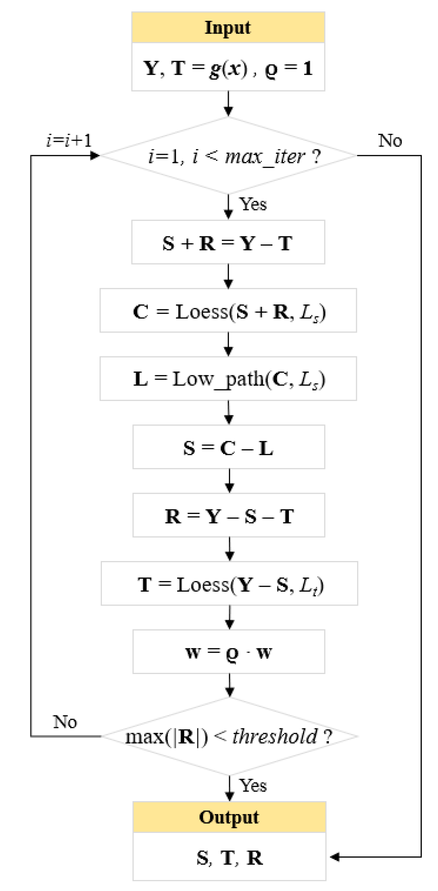
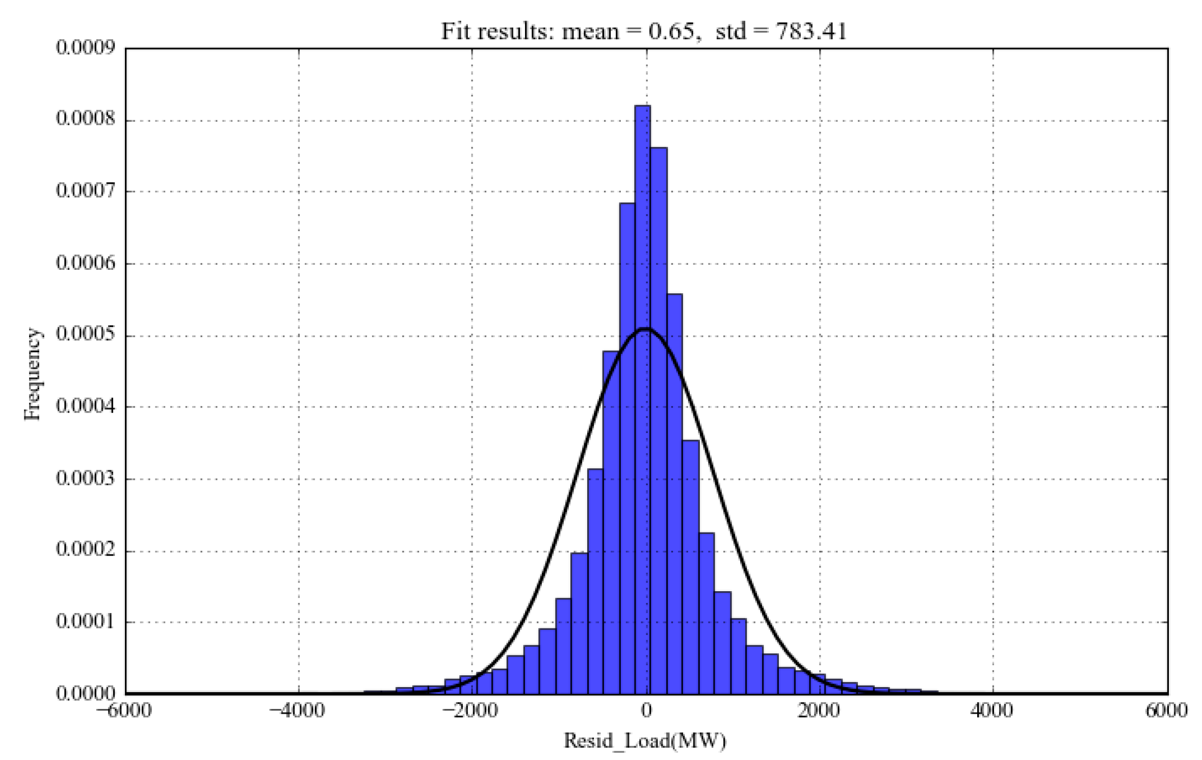
In this paper, a hybrid forecasting framework is proposed focusing on the abnormal load variations in urban cities. First, seasonal and trend decomposition using Loess (STL) [27] is implemented to process the original load series. STL is a classical time series analysis method that can decompose the target series into trending, seasonal, and residual components, which is particularly suitable for power load analysis because power load series naturally has multi-cyclical characteristics. After STL decomposition, the abnormal load variation events can be defined based on the residual component representing irregular load changes. 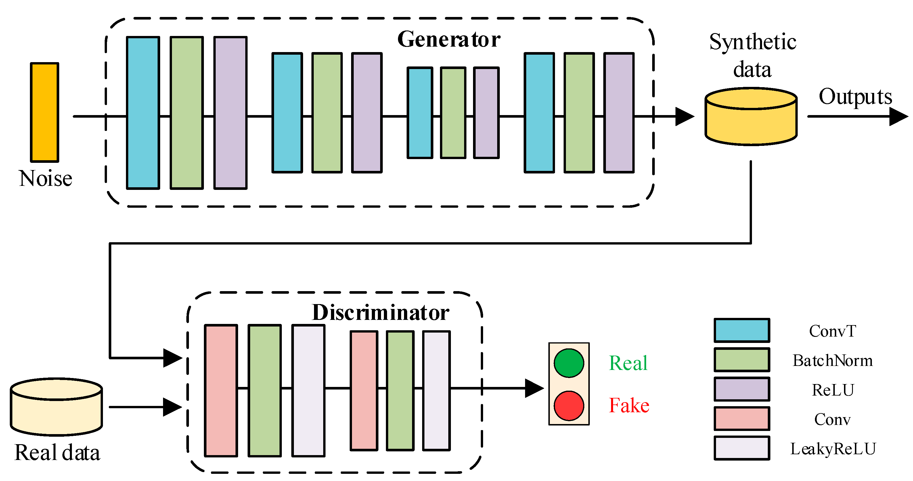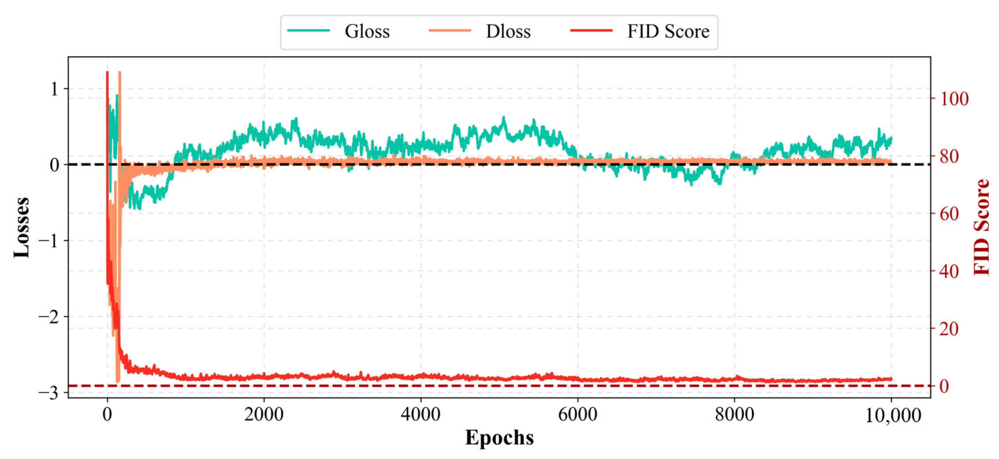Second, Wasserstein Generative Adversarial Nets with Gradient Penalty (WGAN-GP) [28] is introduced to boost the limited number of abnormal load variation samples to a larger quantity to solve the sample scarcity issue. Compared with the vanilla GAN model, WGAN-GP can learn the implicit distribution from the limited abnormal load variation samples to create unlimited synthetic samples, while maintaining a more stable training process and avoiding mode collapse. 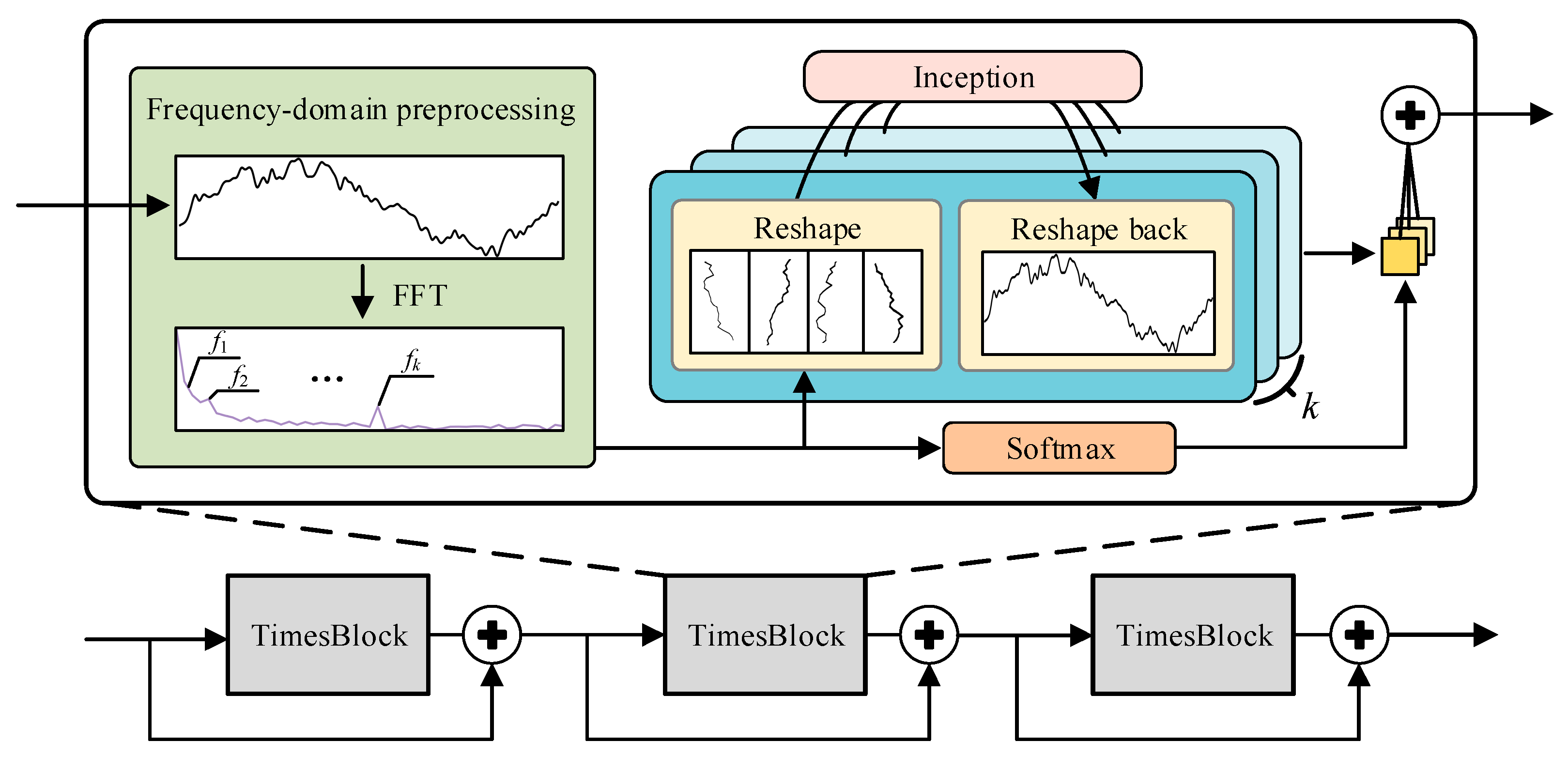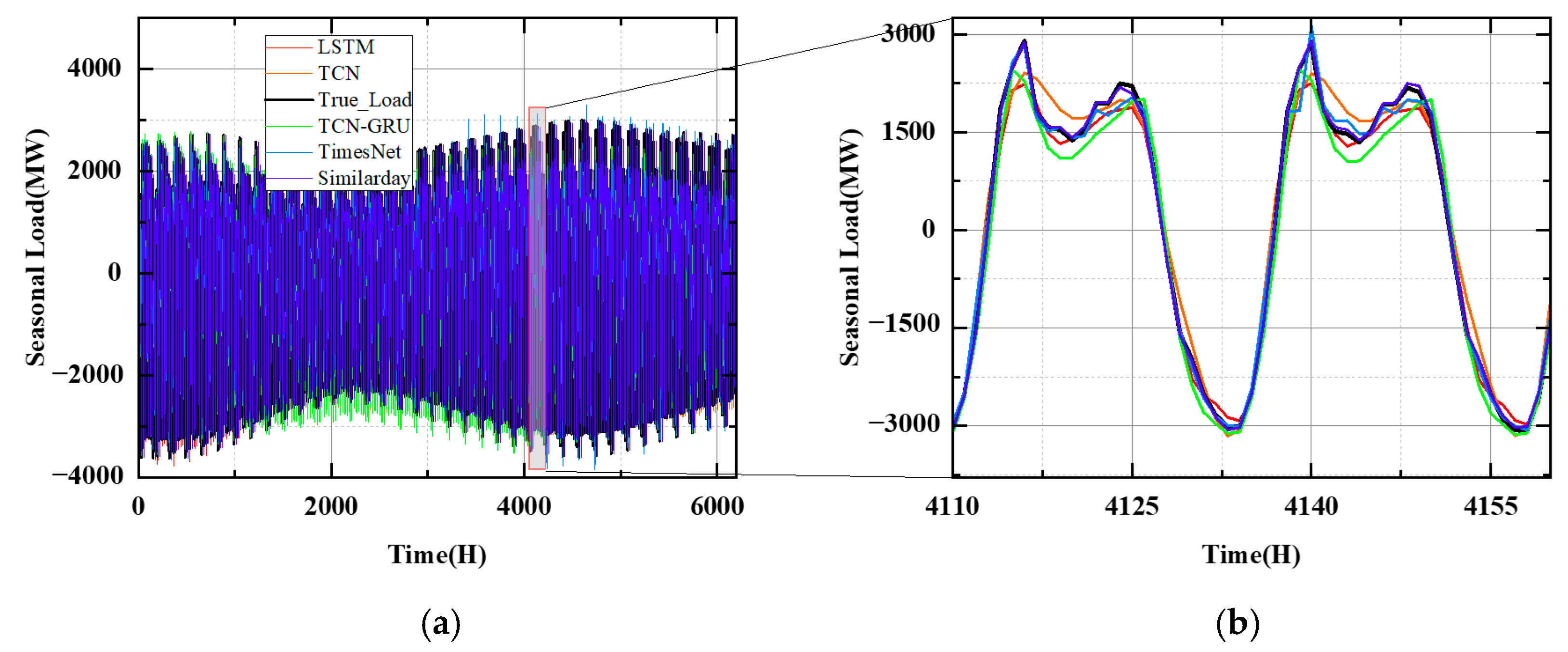Last, to better capture the complex and nonlinear load patterns during abnormal load variation periods, an advanced neural network structure, TimesNet [29], is introduced as the major forecasting model. TimesNet analyzes the load series from the frequency domain to identify the main frequency components and then reshapes the series accordingly to learn both intra-cyclical and cross-cyclical load patterns. Such a learning process is consistent with the multi-cyclical characteristics of the power load, enabling TimesNet to learn complex load patterns during abnormal variation periods.

The major contributions and originalities of this paper are as follows:

(1)

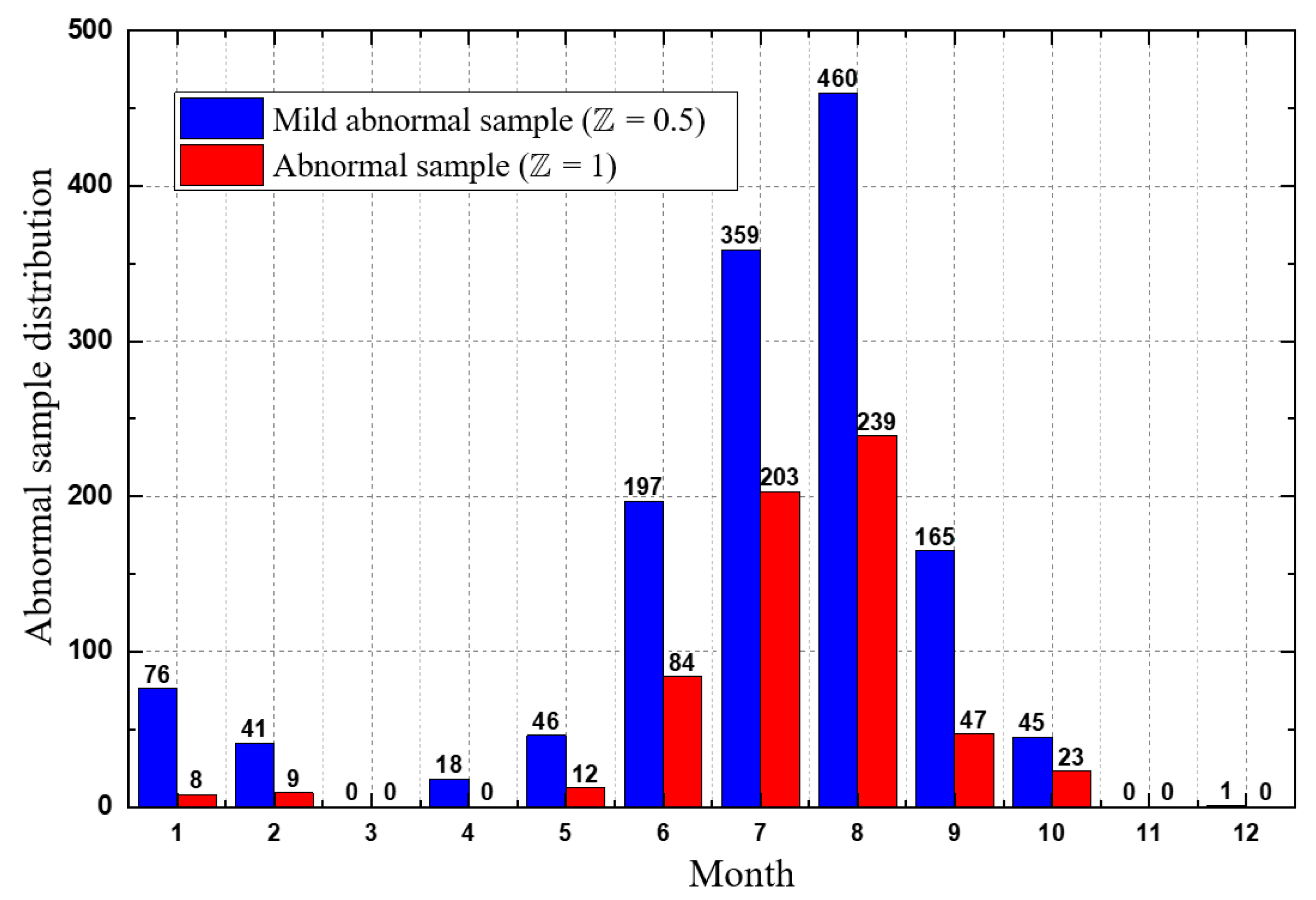
A quantitative method of defining and characterizing abnormal load variation events is proposed. Based on the residual component after STL decomposition, the abnormal events can be identified as the samples locating at the tail part of the residual probability distribution, which indicates low occurrence probability. Then, a quantitative feature can be derived to reflect the abnormity of the load samples according to their occurrence probability, which can be further used to assist the forecasting model training. Such a methodology of defining and characterizing abnormal load variation events is considered original in this paper.

(2)

A customized forecasting framework targeting abnormal load variation forecasting is proposed. Compared with normal load forecasting methods, the proposed framework combines a definition and characterization process of abnormal load variation events, a sample augmentation process to solve the sample scarcity issue, and a state-of-the-art neural network structure as the forecaster, making it customized to the abnormal load variation forecasting problem. To the best of the authors’ knowledge, such a customized and hybrid forecasting framework targeting at abnormal load forecasting has rarely been reported in the existing literature.

The rest of this paper is organized as follows: Section 2 introduces the methodology, Section 3 demonstrates the case study results, and Section 4 concludes this paper.

2. Methodology

The flowchart of the proposed abnormal load variation forecasting framework is summarized in Figure 2. The historical load series is first decomposed into trend, seasonal, and residual components by STL. Then, the abnormal load variation events are identified based on the residual component, the samples of which are further augmented to a larger quantity to enhance the forecasting model training. Finally, each of the trend, seasonal, and residual components are forecasted individually by TimesNet and aggregated to obtain the final forecasting results. Due to the augmented abnormal load variation samples and the powerful learning capability of TimesNet, the proposed forecasting framework can better capture the patterns during abnormal load variation periods, so that the corresponding forecasting accuracy can be improved.

2.1. STL Algorithm for Load Profile Decomposition

The seasonal–trend decomposition procedure based on Loess (STL) is a time series decomposition algorithm particularly suitable for time series’ with a clear trend and seasonal features [27]. For the power load time series Y, the STL algorithm can be summarized as

$$\mathbf{Y}=\mathbf{T}+\mathbf{S}+\mathbf{R}$$

(1)

where T is the low-frequency trending component, S is the high-frequency seasonal component, and R is the residual component representing irregular load variations.

STL is achieved primarily based on the Locally Weighted Regression (Loess) process, defined as function g(·). Assume x is the independent variable series of Y. For any x₀ ∈ x, assume there are q samples within the neighborhood of x₀, denoted as x_i (i = 1, 2, …, q). Then, the weight for the ith sample is given by the tricube weighting function

$$w_i=\left\{\begin{array}{ll}{(1-u^3)}^3,& 0\le u<1\\ \hfill 0,\hfill & u\ge 1\end{array}\right.$$

(2)

$$u={\displaystyle \frac{\left|x_i-x_0\right|}{{\lambda }_q(x_0)}}$$

(3)

where λ_q(x₀) = max(|x₀ − x_i|), i = 1, 2, …, q is the maximum distance between x₀ and all its q neighbors. Then, the estimation for y₀, denoted as ${\widehat{y}}_0$, can be established locally within the neighborhood of x₀ by weighted polynomial fitting, based on the q datum samples (x_i, w_i):

$${\widehat{y}}_0=g(x_0)={\beta }_0+{\beta }_1{x}_0+{\beta }_2{x}_0^2+\cdots +{\beta }_D{x}_0^D$$

(4)

where β₀, β₁,…, β_D are the coefficients that can be obtained by weighted least square regression based on the q neighboring samples of x₀; D is the predefined polynomial order.

Implementing STL in load decomposition includes the following key steps:

(1)

Initialization. Implement the Loess to the original load profile Y to obtain the trending component T = g(x). Seasonal component S is initialized by averaging every L_s samples in Y, and the residual component is initialized by R = Y − S − T. The weighting correction vector ρ is initialized by unit vector.

(2)

Detrending. Subtracting T from Y to obtain the detrended series including seasonal component and residual component.

(3)

Smoothing the detrended series. Implement Loess to each segment of the detrended series to obtain the smoothed version of the detrended series. To smooth out the junctions between segments, Loess will implement again to the whole smoothed detrended series to obtain the final smoothed detrended series C.

(4)

Seasonal component estimation. Because C still contains a low-frequency component, in this step, the low-frequency component in C is further estimated and removed, noted as L, to obtain the final seasonal component S = C − L. L can be obtained by implementing low-path filter to C, which is designed as a moving average process with seasonal window length L_s.

(5)

Residual estimation. The residual component can be calculated as R = Y − T − S.

(6)

Trending component re-estimation. The trending component will be re-estimated by implementing Loess smoothing with window length L_t to the seasonal-free series Y − S.

(7)

Loess weighting correction. To reduce the residual values, a correction vector ρ will be calculated to multiply with the original weighting vector w to update w, shown as Equations (5)–(7). h is the medium value of the residual times 6; B(·) is the squared weighting function. After weighing correction, large residual values will be given with higher weights, so that they can be better reduced in the next iteration.

$$\mathit{\rho }=B({\displaystyle \frac{\left|\mathbf{R}\right|}{h}})$$

(5)

$$B(u)=\left\{\begin{array}{cc}{(1-u^2)}^2& 0\le u<1\\ \hfill 0\hfill & u\ge 1\end{array}\right.$$

(6)

$$h=6\times median(\left|\mathbf{R}\right|)$$

(7)

Note that the above steps (2)–(7) will be executed repeatedly until R is smaller than a given threshold to ensure decomposition effectiveness. T obtained in the previous iteration will serve as the initialization in the current iteration. The flowchart and pseudocode of the above STL decomposition algorithm are shown in Figure 3 and Algorithm 1.

Algorithm 1: STL decomposition algorithm

2.2. Abnormal Load Variation Identification and Characterization

Based on the STL decomposition results, the trending component is interpreted as the long-term load growth, which is correlated with factors such as economic growth, population increase, climate change, etc. The seasonal component is interpreted as the load patterns driven by periodic factors such as season change. Both the trending and seasonal components have clear patterns. On the contrary, the residual component is considered representing load variations caused by irregular factors such as weather change, social events, or user behavior randomness. Therefore, in this paper, the abnormal load variations can be identified and characterized based on the residual component.

Considering the residual component does not have clear pattern and performs as random noise, Gaussian distribution is used to model the residual component, shown as Equations (8)–(10). N is the length of the decomposed residual series R; r ∈ R; μ_r and σ_r are the mean and standard deviation of the fitted Gaussian distribution G(r).

$${\mu }_r={\displaystyle \frac{1}{N}}{\displaystyle \sum _{i=1}^N{r}_i}$$

(8)

$${\sigma }_r=\sqrt{{\displaystyle \frac{1}{N}}{\displaystyle \sum _{i=1}^N{(r_i-{\mu }_r)}^2}}$$

(9)

$$G(r)={\displaystyle \frac{1}{{\sigma }_r\sqrt{2\pi }}}{e}^{-{\displaystyle \frac{{(r-{\mu }_r)}^2}{{2{\sigma }_r}^2}}}$$

(10)

Based on G(r), a discrete feature ℤ is defined to quantify different levels of abnormal load variations:

• Severe abnormal load variation: when r ∈ (−∞, μ_r − 3σ_r] ∪ [μ_r + 3σ_r, +∞), it means the load variations are rare and significant and are far from normal load variation range. Such significant load variations are usually caused by extreme weather conditions or significant social events and are hard to forecast. In this scenario, ℤ is set to 1.
• Mild abnormal load variation: when r ∈ (μ_r − 3σ_r, μ_r − 2σ_r] ∪ [μ_r + 2σ_r, μ_r + 3σ_r), it means the load variations are abnormal but are relatively less severe and rare compared with the first scenario. ℤ is set to 0.5 in this scenario.
• Normal load variation: when r ∈ (μ_r − 2σ_r, μ_r + 2σ_r), it means the load variations are minor and are considered as normal load variations. Such variations are usually caused by daily random factors such as human behavior randomness, production schedule changes, equipment failure or maintenance, etc., and will not cause significant bias to the forecasting results. ℤ is set to 0 in this scenario.

The defined feature ℤ can serve as an additional input feature for the follow-up load forecasting models to assist the model to pay more attention to the abnormal load variation scenarios, so that the forecasting performance in such scenarios can be improved.

2.3. Abnormal Load Variation Sample Augmentation

To solve the sample scarcity issue during the abnormal load variation forecasting, Generative Adversarial Networks (GANs) [30]. are introduced to augment the limited number of abnormal load variation samples to a larger quantity before training the forecasting model.

As illustrated in Figure 4, a GAN model comprises two principal components: a generator (G) and a discriminator (D). The generator network takes a latent vector z as the input, which is typically sampled from a Gaussian noise distribution, to generate diversified synthetic samples $\widehat{\mathbf{x}}=G(\mathbf{z})$ that follow identical distributions with the real samples x. The discriminator network classifies inputs from both the real data distribution x and the generated data $\widehat{\mathbf{x}}$ as either “real” or “fake”. GAN training is a continuous adversarial process between G and D, where the generator seeks to produce data that can deceive the discriminator, and the discriminator attempts to accurately distinguish between real and generated data. This process can be formulated as a minimax problem:

$$\underset{G}{\min }\underset{D}{\max }[{\mathbb{E}}_{\mathbf{x}\in P_r}[\log D(\mathbf{x})]+{\mathbb{E}}_{\widehat{\mathbf{x}}\in P_g}[\log (1-D(\widehat{\mathbf{x}}))]]$$

(11)

where 𝔼 is the expectation operator; P_r and P_g are the probability distributions of real data x and generated data $\widehat{\mathbf{x}}$. To guarantee model training stability and avoid the mode collapse issue that occurs in vanilla GANs, this study adopts the Wasserstein GAN (WGAN) framework, where a Gradient Penalty (GP) method is employed to maintain the Lipschitz constraint during training. The loss function becomes

$$\underset{G}{\min }\underset{D}{\max }[{\mathbb{E}}_{\widehat{\mathbf{x}}\in P_g}[D(\widehat{\mathbf{x}})]-{\mathbb{E}}_{\mathbf{x}\in P_r}[D(\mathbf{x})]]+\lambda {\mathbb{E}}_{\tilde{\mathbf{x}}\in P_{\tilde{\mathbf{x}}}}[{(\parallel {\nabla }_{\tilde{x}}D(\tilde{\mathbf{x}}){\parallel }_2-1)}^2]$$

(12)

where $\tilde{\mathbf{x}}=\epsilon \mathbf{x}+(1-\epsilon )\widehat{\mathbf{x}}$, ε is random number, $P_{\tilde{x}}$ is the probability distribution of $\tilde{\mathbf{x}}$, ∇ is the gradient operator, and λ is a hyperparameter.

Note that the discriminator loss of the WGAN-GP model measures the distance between the real data distribution and the generated data distribution. As a result, the WGAN-GP model is considered converged when the discriminator loss stabilizes around 0, indicating the generated samples follow similar distribution to the real samples. In addition, another independent index, the Fréchet Inception Distance (FID) score, is also introduced to measure the performance of the WGAN-GP as well as validating its convergence:

$$\mathrm{FID}=\left|\right|{\mu }_r-{\mu }_g|{|}^2+\mathrm{Tr}({\mathsf{\Sigma }}_r+{\mathsf{\Sigma }}_g-2{({\mathsf{\Sigma }}_r{\mathsf{\Sigma }}_g)}^{1/2})$$

(13)

where μ_r and μ_g are the mean values of the real and generated samples, ∑_r and ∑_g are the corresponding covariance matrices, and Tr(·) is the operator to calculate the matrix trace. The WGAN-GP model is considered converged when the FID score starts to stabilize around 0.

After the sample augmentation process, both the real and generated samples will be merged into the training set of the forecasting model, so that the forecasting model can pay more attention to the abnormal load variation events and enhance the corresponding forecasting performance.

2.4. TimesNet

In this section, an advanced neural network structure, TimesNet [29], is introduced as the major forecaster to capture complex patterns during abnormal load variation periods. As shown in Figure 5, TimesNet is composed of a series of TimesBlock modules. The details within a TimesBlock includes the following steps:

(1)

Frequency-domain preprocessing. As mentioned above, real-world time series such as the power load can be interpreted as a superposition of multiple components with varying periodicity, making it difficult directly learn. To address this issue, TimesBlock first transforms the original time series into the frequency domain by Fast Flourier Transform (FFT). For a one-dimensional time series (e.g., the power load together with its explanatory variables) X_1D ∈ ℝ^T×C with length T and channel C, its periodicities of different components can be calculated by

$$\mathbf{A}=avg\left(amp\right(FFT({\mathbf{X}}_{1D}\left)\right))$$

(14)

$$f_1,\dots ,f_k=\underset{f\in \{1, \dots , {\displaystyle \raisebox{1ex}{$T$}\!\left/ \!\raisebox{-1ex}{$2$}\right.}\}}{\mathrm{a}\mathrm{r}\mathrm{g}\mathrm{T}\mathrm{o}\mathrm{p}\text{-}k}(\mathbf{A})$$

(15)

$$p_1,\dots ,p_k={\displaystyle \frac{T}{f_1}},\dots ,{\displaystyle \frac{T}{f_k}}$$

(16)

where FFT(·) denotes the FFT function, amp(·) denotes the calculation function of the amplitudes of each frequency component, and avg(·) denotes the averaging function across different channels. After the amplitude vector A is calculated, the frequency components having the top-k amplitudes can be identified and denoted as {f₁, …, f_k}. Accordingly, the period of each component can be calculated by (16) and denoted as {p₁, …, p_k}.

(2)

Reshaping time series into 2D tensors. Based on the periods of the top-k components {p₁, …, p_k}, the original 1D time series X_1D can be reshaped into multiple 2D tensors:

$${\mathbf{X}}_{2D}^i=Reshap{e}_{[p_i,f_i,C]}(Padding({\mathbf{X}}_{1D})),\hspace{1em}i\in \{1,\cdots ,k\}$$

(17)

where Padding(·) extends X_1D by zeros along the temporal dimension to make it capable of being reshaped to the size of [p_i, f_i, C]. Then, the set of 2D tensors {${\mathbf{X}}_{2D}^1$, ${\mathbf{X}}_{2D}^2$, …,${\mathbf{X}}_{2D}^k$} can be obtained with their rows and columns representing the intra-period variation and inter-period variations, respectively.

(3)

Feature extraction by Inception network. The Inception network [31], which is composed of 2D convolution layers, is introduced to learn the multi-periodic information from the 2D tensors:

$${\widehat{\mathbf{X}}}_{2D}^i=Inception({\mathbf{X}}_{2D}^i)$$

(18)

where ${\widehat{\mathbf{X}}}_{2D}^i$ is the extracted feature map that has the same size as the input 2D tensors.

(4)

Reshaping feature map back to 1D series. The extracted feature map ${\widehat{\mathbf{X}}}_{2D}^i$ is transformed back into a one-dimensional series for further aggregation.

$${\widehat{\mathbf{X}}}_{1\mathrm{D}}^i=Trunc(Reshap{e}_{[1, p_i\times f_i]}({\widehat{\mathbf{X}}}_{2D}^i)),\hspace{1em}i\in \{1,\cdots ,k\}$$

(19)

where Trunc(·) represents the function to remove the extended zeros by Padding(·).

(5)

Adaptive aggregation. The obtained 1D feature series ${\widehat{\mathbf{X}}}_{1D}^i$, i ∈ {1, 2, …, k}, are aggregated into a single series weighted by the amplitude vector A representing their frequency-domain intensity.

$${\widehat{\mathbf{X}}}_{1\mathrm{D}}={\displaystyle \sum _{i=1}^k\frac{\mathbf{A}[i]}{‖\mathbf{A}‖}\times {\widehat{\mathbf{X}}}_{1\mathrm{D}}^i}$$

(20)

In practice, multiple TimesBlocks will be concatenated to formulate the whole TimesNet framework. The output feature series ${\widehat{\mathbf{X}}}_{1\mathrm{D}}$ of the (l-1)^th TimesBlock will become the input of the lth block, so that the temporal features of the original power load series can be fully captured. Meanwhile, a residual connection is introduced between two adjacent TimesBlocks to enhance the model performance especially when the network is deep:

$${\mathbf{X}}_{1\mathrm{D}}^l=TimesBlock({\mathbf{X}}_{1D}^{l-1})+{\mathbf{X}}_{1D}^{l-1}$$

(21)

3. Results

3.1. Test Case Setup

The test case in this paper was set up based on the historical load and weather data in Chongqing, China. The historical data are from 1 January 2020 to 23 August 2023 with hourly resolution, plotted as Figure 6. Abnormal variations can be visually identified especially in summer and winter seasons when the air conditioning load takes a significant proportion. The forecasting problem was set up using the previous 24 h historical load and weather data to forecast the next 24 h load profile to support day-ahead system dispatch [32]. The historical data were split into 70% training set and 30% testing set to evaluate the forecasting model’s performance.

To benchmark the proposed TimesNet model, another three deep-learning models were tested, including Long Short-Term Memory (LSTM) [33], Temporal Convolutional Nets (TCN), and TCN combined with Gated Recurrent Nets (TCN-GRU). The model hyperparameter configurations are shown in

Table 1. Model hyperparameter configurations.

Model	Hyperparameter Configurations
LSTM	3 hidden layers, 48 neurons, 0.1 dropout ratio, Adam optimizer, MSE loss function
TCN	2 layers, 3 kernel size, 64 convolution kernels, [1, 2] dilation rate, 0.3 dropout ratio, Adam optimizer, MSE loss function
TCN-GRU	2 TCN layers, 3 kernel size, 64 convolution kernels, [1, 2] dilation rate, 2 GRU layers, 96 neurons, 0.2 dropout ratio, 0.0001 learning rate, Adam optimizer, MSE loss function
TimesNet	6 encoder layers, 1 decoder layer, 256 neurons, 0.1 dropout ratio, 0.0001 learning rate, Adam optimizer, MSE loss function

, under which the models have the best forecasting accuracy after trial-and-error experiments. Meanwhile, the similar day method was also established by using the load profiles in the previous 24 h as the forecasting results for the next 24 h, which served as a baseline.

To evaluate forecasting performance, five quantitative metrics were introduced: Mean Squared Error (MSE), normalized MSE (nMSE), Mean Absolute Error (MAE), normalized MAE (nMAE), and Mean Absolute Percentage Error (MAPE) [34]. The two normalized metrics nMSE and nMAE can avoid the near-zero issue that may occur in MAPE. For simplicity, only the forecasting results of the first hour in the 24 h forecasting window are plotted and calculated.

3.2. Direct Load Forecasting

In this section, the forecasting model performances are evaluated by directly implementing the forecasting model to the original historical series without STL decomposition, abnormal variation identification, and sample augmentation. The results can be used to benchmark model performance as well as serve as a comparison to demonstrate the effectiveness of the proposed forecasting framework in the next few sections. The forecasting results for the testing set are demonstrated in Figure 7 and

Table 2. Summary of the direct load forecasting accuracies.

Metrics	LSTM	TCN	TCN-GRU	TimesNet	Similar Day
MSE(MW2)	1,002,757	978,383	896,066	649,335	846,459
nMSE	0.084	0.082	0.075	0.055	0.068
MAE(MW)	709	696	680	490	556
nMAE	0.051	0.050	0.049	0.035	0.040
MAPE(%)	4.88	4.87	4.72	3.33	3.86

.

From Table 2, it can be seen that TimesNet has the best performance on all metrics, showing 1.55% improvement over LSTM, 1.53% over TCN, and 1.39% over TCN-GRU. Meanwhile, it can also be noticed that the simplest similar day model has good performance in the direct forecasting case, considering that the city-level load profiles usually show evident similarity between two adjacent calendar days.

3.3. STL Decomposition and Forecasting

In this section, the original load profile is first decomposed into a trending component, seasonal component, and residual component. Each component is forecasted, respectively, and summed up to obtain the final forecasting results. Based on this section, the model performances are further compared in different components, and the effectiveness of the STL decomposition method is evaluated.

The two key parameters during STL decomposition are seasonal window L_s and period L_p. L_s defines the Loess window when calculating the seasonal component. A large L_s will generate smoother seasonal components, while a small L_s leads to more fluctuating results. L_p represents the periodicity of the load profile. A large L_p will generate smoother trending components, while a small L_p will fluctuate more. After trial-and-error experiments, L_s = 25 and L_p = 168 were selected to achieve an optimal balance across different components. The decomposition results for the original load series are shown in Figure 8.

From Figure 8, it can be noticed that the trending component is smooth and can reflect the long-term pattern changes in the original load profile. The seasonal component is highly periodic with the mean value close to 0. Both the trending and the seasonal components have clear patterns without random variation. On the contrary, the residual component is composed of noise signals, which is highly stochastic. Because different components have different patterns, next, each component is forecasted independently and aggregate to obtain the final forecasting results.

(1)

Trending component forecasting

Five forecasting models were implemented to forecast the trending component. The models were trained on the trending component samples of the training set and evaluated on the testing set, shown as Figure 9 and

Table 3. Summary of trending component forecasting accuracy.

Metrics	LSTM	TCN	TCN-GRU	TimesNet	Similar Day
MSE (MW2)	9911	64,877	51,362	435	75,564
NMSE	0.0013	0.0086	0.0068	0.000053	0.0092
MAE (MW)	62	207	141	11	158
NMAE	0.0044	0.015	0.010	0.00082	0.011
MAPE (%)	0.40	1.44	0.94	0.080	1.070

. It can be seen that the introduced TimesNet model shows superior performance on the trending component with an MAPE of 0.08%. Compared with the other four benchmarking models, TimesNet shows a 0.32% ~1.36% MAPE improvement, demonstrating superior capability in capturing the long-term load trend.

(2)

Seasonal component forecasting

Following similar a process to the trend component forecasting, the seasonal component forecasting results are summarized in Figure 10 and

Table 4. Summary of seasonal component forecasting accuracy.

Metrics	LSTM	TCN	TCN-GRU	TimesNet	Similar Day
MSE (MW2)	157,186	182,484	95,018	98,102	141,784
NMSE	0.050	0.058	0.030	0.032	0.046
MAE (MW)	289	331	244	197	258
NMAE	0.18	0.21	0.16	0.13	0.16

. Note that because the seasonal component has a close-to-zero mean value, the MAPE metric is not considered when evaluating the model performances due to the zero-denominator issue. Results show that TCN-GRU and TimesNet perform significantly better than the other three models.

(3)

Residual component forecasting

The residual component reflects irregular load variations, among which the weather conditions are the major influencing factor. Therefore, in the residual component forecasting temperature is included as an exogenous variable to enhance the forecasting performance. The forecasting performances are summarized in

Table 5. Summary of residual component forecasting accuracy.

Metrics	LSTM	TCN	TCN-GRU	TimesNet	Similar Day
MSE (MW2)	467,428	517,234	462,912	454,757	577,822
NMSE	0.58	0.64	0.57	0.56	0.86
MAE (MW)	445	473	440	413	434
NMAE	0.72	0.76	0.71	0.67	0.76

and Figure 11. The advantage of TimesNet model is still observable.

(4)

Total load forecasting results

After aggregating the forecasting results of the trending component, seasonal component, and residual component, the total load forecasting results were obtained, as shown in Figure 12 and

Table 6. Summary of total load forecasting accuracy.

Metrics	LSTM	TCN	TCN-GRU	TimesNet	Similar Day
MSE (MW2)	627,577	881,442	663,031	542,877	846,459
NMSE	0.052	0.074	0.056	0.044	0.068
MAE (MW)	557	721	562	467	556
NMAE	0.040	0.051	0.040	0.034	0.040
MAPE (%)	3.86	4.34	3.91	3.24	3.86

.

It can be observed that the TimesNet model still shows the best performance. From Section 3.3, it can be concluded that the proposed TimesNet model has stable and superior performance when forecasting different types of load series. As a result, in the follow-up sections, the TimesNet model becomes the focus and is further tested to improve the forecasting accuracy.

3.4. Forecasting After Abnormal Load Variation Characterization and Sample Augmentation

To make the forecasting model focus on abnormal load variation periods, abnormal load variation events were first identified and characterized based on the criterion in Section 2.2. As shown in Figure 13, probabilistic distribution of the residual component was fitted, and the mean and standard deviation values were obtained. The characterization results are shown in Figure 14. The samples between upper bound 1 and lower bound 1 (dark grey area) are considered normal variations and are assigned ℤ = 0. The samples between upper bound 1 and upper bound 2 as well as between lower bound 1 and lower bound 2 (light grey area) are considered mild abnormal and are assigned ℤ = 0.5. The rest of the samples (white area) are considered abnormal and are assigned ℤ = 1. Based on such definition, ℤ can then be incorporated in the forecasting model inputs as an additional ancillary variable to help the model pay attention to abnormal load variations.

In addition, considering that the abnormal load variation samples take a minor proportion in the total samples, these abnormal samples were augmented to a larger quantity based on the method in Section 2.3 to further enhance the forecasting model training. As shown in Figure 15, 625 abnormal samples (ℤ = 1) and 1408 mild abnormal samples (ℤ = 0.5) were identified in the historical load profile. It can be noticed that that most abnormal variations occur in summer due to drastic temperature impacts. Each abnormal sample was then formulated in a forecasting-oriented data format, in which the abnormal sample was included in the 24 h forecasting horizon paired with 24 h input data. Each sample was also paired with temperature as the exogenous variable.

Then, the WGAN-GP model based on the identified abnormal samples was trained to learn the distribution. To evaluate the model convergence, the generator loss (Gloss), discriminator loss (Dloss), the FID score were recorded and plotted out along with the model training process within 10,000 epochs, as shown in Figure 16. It can be noticed that after around 1000 epochs, both the discriminator loss and the FID score start to stabilize around 0, indicating the model is well converged and the distribution of the generated samples is close to the distribution of the real samples. The FID score at the 1000th epoch is 0.0028.

After the WGAN-GP model was trained and converged, another 2000 synthetic samples were generated. The distributions of the actual abnormal samples and the generated synthetic samples are shown in Figure 17. It can be seen that the mean and peak distributions of the actual and synthetic samples are closely aligned, indicating that the synthetic samples are realistic.

The generated abnormal samples were then incorporated into the training set of the forecasting model to enhance the model performance in learning abnormal load variations. The residual component forecasting accuracy after including the ℤ feature and sample augmentation are shown in

Table 7. Forecasting accuracy for the residual component.

Metrics	Sample Augmentation	ℤ Included	Baseline
MSE (MW2)	466,827	429,996	454,757
NMSE	0.69	0.53	0.56
MAE (MW)	450	401	413
NMAE	0.81	0.64	0.67

, while the accuracy on abnormal samples is shown in

Table 8. Forecasting accuracy for abnormal load variation samples.

Metrics	Sample Augmentation	ℤ Included	Baseline
MSE (MW2)	2,086,058	2,739,755	3,411,852
NMSE	0.43	0.51	0.63
MAE (MW)	1172	1263	1344
NMAE	0.54	0.56	0.60

. It can be seen that by including the defined ℤ feature, TimesNet’s forecasting performance on the residual component is improved. However, when further incorporating the augmented samples into the training set, TimesNet’s performance on the residual component is slightly degraded but is improved on the abnormal load variation samples. Compared with the baseline, the MSE on the residual component increases by 2.65%, while the MSE on the abnormal samples significantly decreases by 38.86%.

4. Discussion

The case study in Section 3 above was designed following the controlled experiment principle to validate the effectiveness of the proposed hybrid forecasting framework part by part. More specifically:

• The advantage of the introduced TimesNet forecaster can be validated by comparing its forecasting accuracy with other benchmarking models under different forecasting scenarios. Note that although in most cases TimesNet shows better accuracy, its advantages over benchmarking models still vary significantly. For example, in trend component forecasting, TimesNet shows extremely high accuracy with only 0.08% MAPE (see Table 3), overwhelmingly beating benchmarking models. However, in seasonal component forecasting, TimesNet is slightly worse than the TCN-GRU model (see Table 4). This indicates that TimesNet is comparably more suitable for smooth series modeling and forecasting, instead of a volatile series.
• As discussed in much of the existing literature, it is a practical and effective strategy to decompose the original load series into different components and conduct modeling/forecasting, respectively, to obtain the final forecasting results. Such conclusion can be supported by comparing the results in Table 2 and Table 6. All machine learning models have considerable accuracy improvements under such a decompose–forecast–aggregation strategy, compared with a direct forecasting strategy. This is because each component has a more evident pattern and is easier to learn than directly learning the total load pattern, which is essentially a superposition of multiple sub-patterns.
• As shown in Table 7 and Table 8, introducing the augmented abnormal load samples can improve the forecasting accuracy during abnormal load periods, but will lead to accuracy decrease in all periods. This is easy to understand, as introducing synthetic abnormal samples will increase the proportion of the abnormal samples in the total set of samples, driving the machine learning model to pay more attention to the abnormal load pattern that is significantly different from the normal pattern. This showed us that when introducing synthetic samples to the total dataset, it is important to find an optimal balance between the accuracy improvement in the augmented scenario and the accuracy loss in other scenarios.

We also noticed that, based on the case study results, the proposed forecasting framework still has some limitations that need to be further addressed:

• The causes of abnormal load variations are not traceable. The proposed abnormal load identification method is solely based on the shape characteristics of the load profile without analyzing the reason. In such cases, although 625 abnormal load variations were identified, it is not clear which factors cause such abnormal variation, prohibiting more in-depth modeling and analysis. In future study, it is suggested to collect more exogeneous variable data and conduct cause–effect analysis to better understand abnormal load variations, which may further benefit forecasting.
• The defined variable ℤ is given in a discrete form (0, 0.5, 1) to quantify the abnormality of the load series. However, such a discrete quantification method is a bit too rough to reflect the actual abnormality of a load series. For example, two abnormal samples with ℤ = 1 may have very different patterns. A continuous quantification method might be a better solution in future study.
• There are subjectivities in the proposed methodology that may influence forecasting performance. For example, the STL decomposition results are highly sensitive to hyperparameters such as seasonal window L_s and period window L_p, the selection of which is empirical. Also, the neural network forecaster and the abnormal event quantification method both include an empirical setup that highly relies on human experience. Considerable trial-and-error efforts may be required to tune the whole framework to obtain satisfying performance.

5. Conclusions and Future Work

In this paper, a hybrid forecasting framework focusing on improving load forecasting accuracy in urban cities during abnormal load variation periods is proposed. This framework includes a definition and characterization process of abnormal load variation events, a sample augmentation process to solve the sample scarcity issue, and a state-of-the-art neural network, TimesNet, as the forecaster, making it highly customized and suitable for abnormal load variation forecasting. Experiments are conducted based on 3-year historical load and weather data in Chongqing, China with the following major results obtained: (1) Based on the proposed abnormal load definition method, 625 abnormal load variation events and 1408 mild abnormal events are successfully identified among the 3-year historical load profile. By characterizing these abnormal events as a quantitative feature and incorporating the feature into the forecasting model input, the forecasting accuracy of the residual component can be improved by 5.44% for the whole testing set and by 19.70% for the abnormal samples. Such an observation demonstrates the effectiveness of the proposed abnormal load definition and characterization method in improving abnormal load forecasting accuracy. (2) Based on the identified 625 abnormal samples, another 2000 synthetic abnormal samples are generated to assist the forecasting model training. Results show that the forecasting accuracy for the abnormal samples is significantly improved by 38.86% with only 2.65% accuracy decrease on the whole testing set. Both major results formulate a controlled experiment, demonstrating the effectiveness of the proposed hybrid forecasting framework.

Future work is suggested to focus on the following aspects: First, the impact of significant social events, such as large-scale social activities and impactful policy implementation, can be analyzed to quantify their impact on urban power load to enhance forecasting. Second, few-shot learning techniques can be further explored to solve the sample scarcity issue in the abnormal load variation forecasting problem. Third, modeling of user consumption behavior can be further detailed, so that load forecasting can be accurately achieved by aggregating user consumption simulation results.

References

1. Pecan Street. Available online: https://www.pecanstreet.org (accessed on 11 December 2024).
2. Time and Date. Available online: https://www.timeanddate.com/weather/usa/austin (accessed on 5 November 2024).
3. Fay, D.; Ringwood, J.V. On the influence of weather forecast errors in short-term load forecasting models. IEEE Trans. Power Syst. 2010, 25, 1751–1758. [Google Scholar] [CrossRef]
4. Chu, W.C.; Chen, Y.P.; Xu, Z.W.; Lee, W.-J. Multiregion short-term load forecasting in consideration of HI and load/weather diversity. IEEE Trans. Ind. Appl. 2010, 47, 232–237. [Google Scholar] [CrossRef]
5. Yu, B.; Li, J.; Liu, C.; Sun, B. A novel short-term electrical load forecasting framework with intelligent feature engineering. Appl. Energy 2022, 327, 120089. [Google Scholar] [CrossRef]
6. Wang, Y.; Zhang, N.; Chen, X. A short-term residential load forecasting model based on LSTM recurrent neural network considering weather features. Energies 2021, 14, 2737. [Google Scholar] [CrossRef]
7. Xie, J.; Chen, Y.; Hong, T.; Laing, T.D. Relative humidity for load forecasting models. IEEE Trans. Smart Grid 2016, 9, 191–198. [Google Scholar] [CrossRef]
8. Hong, T.; Wang, P.; White, L. Weather station selection for electric load forecasting. Int. J. Forecast. 2015, 31, 286–295. [Google Scholar] [CrossRef]
9. Mansouri, A.; Abolmasoumi, A.H.; Ghadimi, A.A. Weather sensitive short term load forecasting using dynamic mode decomposition with control. Electr. Power Syst. Res. 2023, 221, 109387. [Google Scholar] [CrossRef]
10. Xie, J.; Hong, T. Temperature scenario generation for probabilistic load forecasting. IEEE Trans. Smart Grid 2016, 9, 1680–1687. [Google Scholar] [CrossRef]
11. Dehalwar, V.; Kalam, A.; Kolhe, M.L.; Zayegh, A. Electricity load forecasting for Urban area using weather forecast information. In Proceedings of the IEEE: 2016 IEEE International Conference on Power and Renewable Energy (ICPRE), Shanghai, China, 21–23 October 2016; IEEE: Piscataway, NJ, USA, 2016; pp. 355–359. [Google Scholar]
12. Lu, Q.; Cai, Q.; Liu, S.; Yang, Y.; Yan, B.; Wang, Y. Short-term load forecasting based on load decomposition and numerical weather forecast. In Proceedings of the IEEE: 2017 IEEE Conference on Energy Internet and Energy System Integration (EI2), Beijing, China, 26–28 November 2017; IEEE: Piscataway, NJ, USA, 2017; pp. 1–5. [Google Scholar]
13. Xu, L.; Wang, S.; Tang, R. Probabilistic load forecasting for buildings considering weather forecasting uncertainty and uncertain peak load. Appl. Energy 2019, 237, 180–195. [Google Scholar] [CrossRef]
14. Kim, Y.; Son, H.; Kim, S. Short term electricity load forecasting for institutional buildings. Energy Rep. 2019, 5, 1270–1280. [Google Scholar] [CrossRef]
15. Li, B.; Lu, M.; Zhang, Y.; Huang, J. A weekend load forecasting model based on semi-parametric regression analysis considering weather and load interaction. Energies 2019, 12, 3820. [Google Scholar] [CrossRef]
16. Pinheiro, M.G.; Madeira, S.C.; Francisco, A.P. Short-term electricity load forecasting—A systematic approach from system level to secondary substations. Appl. Energy 2023, 332, 120493. [Google Scholar] [CrossRef]
17. Guo, H.; Huang, B.; Wang, J. Probabilistic load forecasting for integrated energy systems using attentive quantile regression temporal convolutional network. Adv. Appl. Energy 2024, 14, 100165. [Google Scholar] [CrossRef]
18. Chen, Y.; Zhang, D. Theory-guided deep-learning for electrical load forecasting (TgDLF) via ensemble long short-term memory. Adv. Appl. Energy 2021, 1, 100004. [Google Scholar] [CrossRef]
19. Li, L.; Ota, K.; Dong, M. When weather matters: IoT-based electrical load forecasting for smart grid. IEEE Commun. Mag. 2017, 55, 46–51. [Google Scholar] [CrossRef]
20. Deng, X.; Ye, A.; Zhong, J.; Xu, D.; Yang, W.; Song, Z.; Zhang, Z.; Guo, J.; Wang, T.; Tian, Y.; et al. Bagging-XGBoost algorithm based extreme weather identification and short-term load forecasting model. Energy Rep. 2022, 8, 8661–8674. [Google Scholar] [CrossRef]
21. Yang, W.; Sparrow, S.N.; Wallom, D.C.H. A comparative climate-resilient energy design: Wildfire Resilient Load Forecasting Model using multi-factor deep learning methods. Appl. Energy 2024, 368, 123365. [Google Scholar] [CrossRef]
22. Zhang, T.; Tang, D.; Fan, P.; Wang, Q.; Wang, P. A Probabilistic Graphical Model for Predicting Cascade Failures of Electric Vehicle Charging Networks Caused by Hurricanes. IEEE Trans. Smart Grid 2024, 16, 627–639. [Google Scholar] [CrossRef]
23. Shield, S.A.; Quiring, S.M.; Pino, J.V.; Buckstaff, K. Major impacts of weather events on the electrical power delivery system in the United States. Energy 2021, 218, 119434. [Google Scholar] [CrossRef]
24. Watson, E.B.; Etemadi, A.H. Modeling electrical grid resilience under hurricane wind conditions with increased solar and wind power generation. IEEE Trans. Power Syst. 2019, 35, 929–937. [Google Scholar] [CrossRef]
25. Kwasinski, A.; Andrade, F.; Castro-Sitiriche, M.J.; O’Neill-Carrillo, E. Hurricane Maria Effects on Puerto Rico Electric Power Infrastructure. IEEE Power Energy Technol. Syst. J. 2019, 6, 85–94. [Google Scholar] [CrossRef]
26. Fatima, K.; Shareef, H.; Costa, F.B.; Bajwa, A.A.; Wong, L.A. Machine learning for power outage prediction during hurricanes: An extensive review. Eng. Appl. Artif. Intell. 2024, 133, 108056. [Google Scholar] [CrossRef]
27. Cleveland, R.B.; Cleveland, W.S.; McRae, J.E.; Terpenning, I. STL: A seasonal-trend decomposition. J. Off. Stat. 1990, 6, 3–73. [Google Scholar]
28. Jin, Q.; Lin, R.; Yang, F. E-WACGAN: Enhanced generative model of signaling data based on WGAN-GP and ACGAN. IEEE Syst. J. 2019, 14, 3289–3300. [Google Scholar] [CrossRef]
29. Wu, H.; Hu, T.; Liu, Y.; Zhou, H.; Wang, J.; Long, M. Timesnet: Temporal 2d-variation modeling for general time series analysis. arXiv 2022, arXiv:2210.02186. [Google Scholar]
30. Goodfellow, I.; Pouget-Abadie, J.; Mirza, M.; Xu, B.; Warde-Farley, D.; Ozair, S.; Courville, A.; Bengio, Y. Generative adversarial networks. Commun. ACM 2020, 63, 139–144. [Google Scholar] [CrossRef]
31. Szegedy, C.; Vanhoucke, V.; Ioffe, S.; Shlens, J.; Wojna, Z. Rethinking the inception architecture for computer vision. In Proceedings of the IEEE Conference on Computer Vision and Pattern Recognition, Las Vegas, NV, USA, 27–30 June 2016; pp. 2818–2826. [Google Scholar]
32. Gao, Y.; Ai, Q. A novel optimal dispatch method for multiple energy sources in regional integrated energy systems considering wind curtailment. CSEE J. Power Energy Syst. 2022, 10, 2166–2173. [Google Scholar]
33. Shang, Y.; Li, D.; Li, Y.; Li, S. Explainable spatiotemporal multi-task learning for electric vehicle charging demand prediction. Appl. Energy 2025, 384, 125460. [Google Scholar] [CrossRef]
34. Feng, C.; Shao, L.; Wang, J.; Zhang, Y.; Wen, F. Short-term load forecasting of distribution transformer supply zones based on federated model-agnostic meta learning. IEEE Trans. Power Syst. 2024, 40, 31–45. [Google Scholar] [CrossRef]
Figure 1. Temperature profile and the aggregated residential load profile in Austin, Texas in August 2017. In the upper subfigure, red and blue ticks represent 24-hour temperature highs and lows. Faint red and blue lines represent the daily average high and low temperatures with 25th to 75th and 10th to 90th percentile bands.
Smartcities 08 00043 g001
Figure 2. Flowchart of the proposed abnormal load variation forecasting framework.
Smartcities 08 00043 g002
Figure 3. Flowchart of the STL decomposition algorithm.
Smartcities 08 00043 g003
Figure 4. GAN framework in this paper.
Smartcities 08 00043 g004
Figure 5. TimesNet framework.
Smartcities 08 00043 g005
Figure 6. Historical data in Chongqing with hourly granularity: (a) load data; (b) temperature data.
Smartcities 08 00043 g006
Figure 7. Direct load forecasting results for the testing set: (a) forecasting result overview of the whole testing set; (b) regional zoom-in of the forecasting results.
Smartcities 08 00043 g007
Figure 8. The original and decomposed load profiles.
Smartcities 08 00043 g008
Figure 9. Trending component forecasting results for the testing set: (a) forecasting result overview of the whole testing set; (b) regional zoom-in of the forecasting results.
Smartcities 08 00043 g009
Figure 10. Seasonal component forecasting results for the testing set: (a) forecasting result overview of the whole testing set; (b) regional zoom-in of the forecasting results.
Smartcities 08 00043 g010
Figure 11. Residual component forecasting results for the testing set: (a) forecasting result overview of the whole testing set; (b) regional zoom-in of the forecasting results.
Smartcities 08 00043 g011
Figure 12. Total load forecasting results for the testing set: (a) forecasting result overview of the whole testing set; (b) regional zoom-in of the forecasting results.
Smartcities 08 00043 g012
Figure 13. Probabilistic distribution fitting results of the residual component.
Smartcities 08 00043 g013
Figure 14. Characterization results of the abnormal load variation events.
Smartcities 08 00043 g014
Figure 15. Distribution of the abnormal load variations throughout the year.
Smartcities 08 00043 g015
Figure 16. The training process of the WGAN-GP model.
Smartcities 08 00043 g016
Figure 17. Distributions of real and synthetic abnormal samples: (a) load distribution; (b) temperature distribution.
Smartcities 08 00043 g017