Coupling of Lagrangian Mechanics and Physics-Informed Neural Networks for the Identification of Migration Dynamics

Highlights

What are the main findings?

• We have developed a dynamic migration model based on the physical principles of Lagrangian mechanics, which enables us to address the limitations of conventional migration models that rely on macroeconomic indicators.
• We investigated the external forces through the physics-informed neural networks in the dynamic equation and explained these forces by using socio-economic indicators.

What is the implication of the main finding?

• Our model can be utilized by administrators in smart cities to evaluate the impact of regional development initiatives or government regulations on the migration patterns of citizens.
• Analyzing the invariant density of transfer operators can assist in determining primary migration directions.

Abstract

An essential aspect of any government in a smart city is to examine the issues of internal and external migration. Migration is a complex phenomenon. In order to effectively manage it, it is not only necessary to be able to accurately predict migration patterns but also to understand which factors influence these patterns. Current approaches to the development of migration models rely on macroeconomic indicators without considering the specificities of intraregional interactions among individuals. In this paper, we propose a method for determining the dynamics of migration balance based on Lagrangian mechanics. We derive and interpret the potential energy of a migration network by introducing specific functions that determine migration patterns. The solution of the migration equations and selection of parameters, as well as external forces, are achieved through the use of physics-informed neural networks. We also use external factors to explain the non-homogeneity in the dynamic equation through the use of a regression model. We analyze settlement priorities using transfer operator theory and invariant density. The findings obtained enable the assessment of migration flows and analysis of external migration factors.

1. Introduction

The primary goals of smart cities are to maximize resource efficiency, foster the use of renewable energy sources, improve safety and environmental standards, optimize the utilization of human resources, and harness the power of AI to process vast amounts of data and manage city infrastructure [1,2]. In smart cities, a key resource is not physical infrastructure or financial capital but rather people. As such, effective city management involves designing communication strategies [3,4] that facilitate the adaptation of the city to social needs and vice versa. This implies that it is feasible to manage migration patterns in a manner that facilitates the access of individuals who necessitate specific areas or cities, while those who do not require such access can relocate to other regions.

In this regard, it is essential that migration-related matters should be automated in all modern states with a view to digitalization and urbanization. Migration enables one to discern the directions of regional development and forecast the appropriate level of investment in a region [5]. In the future, smart cities and smart governments [6] should monitor the preferences of specific regions in real time and adjust the activities of local authorities in order to improve the mood of residents in these areas and foster local economic development.

A smart city can be conceptualized as a complex system comprising numerous decision-making centers that receive a vast amount of diverse information. These centers are compelled to autonomously make decisions to address specific challenges or devise plans for their resolution [7,8]. However, within such a system, there are also subsystems that exhibit complex behavior, such as models of human behavior in society [9,10].

Various approaches exist for modeling migration. The most basic approach is the cellular automata approach. Cellular automata is a mathematical method that can effectively analyze the nonlinear qualities of dynamic human interaction among individuals within a community. Such models can further assist in describing and comprehending urban migration patterns [11,12].

In contrast, when multimodal communications and centers of attraction (cities) are present, cellular automata are not applicable. Therefore, it is crucial to describe the topology of connections, leading to the formation of complex networks.

Complex networks have a significant impact on modern science due to their ability to work with data that relates not only to the individual elements of a system but also to their interactions. The study of complex networks has emerged in various fields, including biology, economics, physics, the social sciences, and chemistry, among others. For example, in biology, the complex networks describe protein–protein interactions [13,14], genetic interaction [15], the brain [16], and metabolic networks [17], among others. The social sciences consider the behavior of a group of people [18] or the community formation [19].

In our article, we are interested in the migration network, which corresponds to a set of settlements and the movement of people between them. The dynamics of migration is a crucial aspect in the studies of government. The interest in this aspect is explained by the economic development of regions. If there is a significant outflow from a particular settlement, it may indicate problems with the development and well-being of its citizens. This could lead the government to increase investments, among other measures.

Firstly, the complexity arises from the number of settlements. For example, in Germany there are approximately two thousand cities, according to the Federal Statistical Office of Germany (https://www.destatis.de/EN/Home, accessed on 15 January 2025). In the United States, about twenty thousand, according to the United States Census Bureau (https://www.census.gov, accessed on 15 January 2025). In Russia, there are around 1100 cities and 1200 urban-type settlements, according to the information from the Federal State Statistics Service (https://eng.rosstat.gov.ru, accessed on 15 January 2025). However, the number of non-city settlements, such as villages, rural areas, or urban-type settlements, may exceed tens of thousands.

Secondly, if we consider the movement of individuals who may travel from their settlement to a neighboring or even a different region of the country, a huge number of combinations of various factors can influence the direction of people’s movement. For instance, an individual’s mobility may be influenced by macroeconomic factors related to the overall regional development [20], economic performance of the country, political decisions [21], urban planning in their area, their emotional state, technological skills [22], their age and family status, as well as the development of neighboring regions [23,24,25].

Migration can be modeled using data-driven models [5,26,27,28], but based on these models, it is challenging to effectively manage such migration. This is because it is crucial to comprehend the interplay between three key elements: (i) the factors that attract individuals to a specific city, (ii) the factors that force individuals to depart from other cities, and (iii) communication. Given the complex nature of the migration network, it cannot be adequately described by employing conventional regression models. Consequently, it is imperative to adopt approaches that combine physical (or cause-and-effect) modeling with data-driven techniques.

In this article, we present a novel approach in migration modeling that integrates Lagrangian mechanics principles to derive the equation of motion. This approach is complemented by a neural network approach to estimate the parameters of the equation and obtain a more precise solution by minimizing deviations from the provided training data. Our technique effectively combines data-driven and physical approaches.

Our contribution is as follows:

(i)

The dynamic migration model is based on a network of locations that are controlled by external factors and its modification using physicalyl-informed neural networks to explain external influences.

(ii)

The method of modeling and forecasting migration using econophysics and Lagrangian mechanics.

(iii)

The method for modeling the priority of settlements for migration through the transfer operators.

(iv)

The explanation of the function responsible for external impacts using regression analysis based on macroeconomic variables.

The remainder of this paper is organized as follows: In the next section, we provide a literature review on the topic under consideration; in Section 3, we propose our dynamic model. We construct the Lagrangian of a system and give the description of its components; in Section 4, we formulate the physics-informed neural network to solve our dynamic equation; in Section 5, we use transfer operators theory to determine the settlement priorities for migration; in Section 6, we evaluate our model by conducting a detailed experimental study on several cases and provide corresponding results with migration network visualization.

2. Related Works

The vast number of articles is devoted to the construction of migration dynamics through macroeconomic factors instead of considering the middle or low level of scale. For example, in work [29], the demographic equation is based on general numbers of births, deaths, inflows, and outflows. Such models have a good approximation of the overall demographic status, but they do not consider the individual levels. The other work [5] considers the macroeconomic and urban factors that influence the migration balance. The authors have demonstrated the influence of average salary, the level of investments in the region, retail turnover, volume of annual construction, and so on. Despite the fact that there are some studies using regression models [30,31,32], all require a certain set of factors.

The academic community is currently struggling with the challenge of identifying the primary factors that drive people to relocate [30]. Despite the extensive discussions on a specific set of factors, the push-and-pull approach remains the most commonly used classification method in various migration studies [25,33]. This approach categorizes all relevant factors into two distinct groups: push factors, which motivate individuals to leave their current location, and pull factors, which attract individuals to specific destinations [25,33,34].

As we previously stated, there are also models that are based on cellular automata [11,12]. Cellular automata are based on the definition of the state of nodes through neighboring cells and their specific characteristics. Migration in such cases occurs when a certain threshold of certain variables is reached.

For instance, a social threshold, which is determined by both the internal state of the household and the external environment. If neighbors all depart for some reason, this can also trigger migration within the current cell [35,36]. To ensure that households do not relocate at every iteration of the model, a probabilistic function is employed to determine when they will migrate. The probability of a move occurring is contingent upon the dissatisfaction of the household with their neighborhood, or in other words, the disparity between their social structure and the average social structure of their neighbors [11]. However, the problem of migration, in its full scope, cannot be tackled with simple approaches like cellular automata due to its complex nature.

Some studies use the agent-based approach to simulate the migration patterns [37,38,39]. For example, the study [38] considers the agents migration from rural to urban areas in economies that are in the early stages of industrialization. The analysis is carried out using a statistical mechanics approach, where the agents are placed on a lattice, and their interactions are described using an Ising-type model.

In [40], the authors review agent-based models of human migration with respect to their decision-making rules. They consider psycho-social and cognitive models and the use of decision theory to describe the complex behavior of people and to interpret the expectations and choices. The problem with agent models lies in the excessive heuristic description of the behavior of these agents, which is usually based on the psychological and social aspects of human behavior.

There are works where the migration pattern is considered through social networks. For example, using spatial econometric techniques, researchers in [41] have demonstrated that strong social connections play a significant role in determining the decision to undertake a first migration. The impact of these connections, however, varies across regions of origin, with some areas experiencing a substantial and positive influence, whereas others do not. In [42], researchers employ complex network theory to address not only social and economic factors but also the utilization of mathematical models in population and migration dynamics. Furthermore, they conduct an indirect influence analysis of these dynamics.

Our article is based on the Lagrangian mechanics principle, which is already used in economic and social modeling. In studies [43,44,45], researchers apply the fundamental principle from physics to construct the Lagrangian and subsequently derive the corresponding dynamic equation. The principles of physics are also applied in the field of sociophysics [46,47,48], employing analogies from physics to describe social and economic phenomena. There are also a number of works where physical models of the type of reaction–diffusion PDE are used to model environmental problems, such as the effect of soil toxicity on plant biomass [49].

Other examples of using physical concepts are based on gravity. The gravity model postulates that the migration flow between two locations is directly proportional to the product of their populations and inversely proportional to the distance between them. Gravity models offer an intuitive framework to comprehend the factors that influence the flow of resources between settlements. However, estimating gravity models necessitates detailed data for country pairs. Analyzing the outcomes of gravity models from a policy standpoint can be difficult due to worries about the accuracy of the data and the impact of other variables [50,51]. Also, such models may not account for unexpected events (e.g., wars, pandemics) that disrupt migration patterns.

3. Model Formulation

3.1. General Formulation of the Problem

Our objective is to analyze the migration patterns of the population within different regions of the country and across the country as a whole. People migrate from one location to another in search of enhanced social and emotional well-being. Social well-being can be influenced by factors such as salary, opportunities for career advancement, access to educational and healthcare facilities, and other aspects. Emotional well-being may be affected by surrounding conditions, such as the presence or absence of harmful industries in the area, the availability of green spaces, and so on. Additionally, emotional well-being is influenced by local amenities such as shopping centers, cinemas, and other recreational facilities.

Internal factors encompass the entire structure of the world for a specific economic agent, and there are numerous such agents within a given locality who interact according to complex rules. This phenomenon is referred to as the micro level. At the macro level, the government allocates funds for the modernization and development of territories, thereby intervening in the environment of these economic agents and attempting to provide them with stimulus.

We encountered several challenges. The formation of specific decisions by economic agents regarding migration to a particular locality remains uncertain. Due to the difficulty in collecting such data, it is infeasible to provide a comprehensive description of the agents’ states.

Furthermore, migration is not a singular event. Individuals may return to their parents or relocate their children to a neighboring settlement, establishing connections with both previous and new locations that are challenging to monitor in the real world. In our model, we rely on data pertaining to official migration, which encompass the framework within which a person registers with local authorities to indicate a change in their place of residence.

Figure 1 illustrates an example of a possible migration network. Each node represents a settlement, and each link represents a road connecting two settlements, indicating the possibility of migration between them. The green color represents the positive migration balance, and the red color represents the negative one. In reality, we do not have information about the precise dynamics of migration at the individual level. Instead, we only know that for a certain settlement $u\in \{1,\cdots ,N\}$, the migration balance was $-200$ individuals, where N is the number of settlements. It means that in a given year, $t_1$, x individuals arrived at the u, but $x+200$ individuals left the settlement. For another example, let us have the information that $R_v\left(t_2\right)=40$, where $R_v$ means the migration balance of the settlement v. It implies that the total difference between the number of people moving to or from v from all other settlements was equal to 40 in the year $t_2$.

Due to the possibility of migration not only within a single region but also to different ones or even different countries, we should consider the establishment of an additional, imaginary city that would absorb all migration balances from other regions. By introducing such a hypothetical city, we would also create a closed system. In Figure 1, we denote the imaginary city in purple. The imaginary city is not located on any map. For visual purposes, we have placed it at the bottom.

For each link (edge) in the migration network, we assign a weight that corresponds to the distance between cities. The value of this weight can be expressed in kilometers or any other unit of measurement, as it simply represents a measure of remoteness. For training purposes, we normalize the weights to the range $[0,1]$.

The distance between settlements is contingent upon the coordinates and is calculated directly from them. Consequently, if an individual migrates by car, the actual distance covered will be greater, as roads rarely correspond to a straight course between two settlements. Despite the convenience of air travel, aircraft frequently encounter turbulence and deviate from a direct course during landing, necessitating a glide path to align with the runway.

Figure 1 also illustrates the factors that influence the in- and out-migration of the population with the teal color. For instance, if a city has a high level of polluting industries, people may choose to relocate to a more eco-friendly city. If there is a lack of employment opportunities in the current location, residents may migrate to another city in search of work.

Our goal is to construct a dynamic model for population migration for an arbitrary region with several settlements using the physical approaches. The number of settlements in the region is equal to N (including the imaginary settlement). For the purpose of this article, we will consider the region to be the union of villages and urban areas. However, it is also possible to view the region as a union of federal states, in which case the region would cover the entire country.

Instead of the absolute number of individuals in the settlements, we consider the migration balance. That is, we are interested in the number of people leaving or arriving in each settlement. Let $R_u\left(t\right)$ be the saldo of the migration (migration balance) for the settlement $u\in I$ at the time moment $t\in T$, where T is the set of indexes that can have a discrete or continuous nature, and $I=\{1,\cdots ,N\}$ is the set of settlement indexes. In our article, the elements of T represent years. The meaning of $R_u\left(t\right)\in \mathbb{Z}$ is the total difference between the number of people who left or arrived at the settlement u at the time t. The unit of measurement is the number of people. For training purposes, it is better to scale the $R_u$ to the range $[-1,1]$ and assume $R_u\left(t\right)\in \mathbb{R}$.

The derivative ${\dot{R}}_u\left(t\right)$ of $R_u\left(t\right)$ is the rate of change in the migration saldo (${\displaystyle \frac{\mathrm{people}}{\mathrm{year}}}$). It represents how quickly people change their location. We denote the vector of saldo by $R=(R_1,\cdots ,R_N)$ and the derivatives vector by $\dot{R}=({\dot{R}}_1,\cdots ,{\dot{R}}_N)$. Our system consists of N generalized coordinates $R_u$, i.e., we have N degrees of freedom. The full state of a system can be described by a set of generalized coordinates R and generalized velocities $\dot{R}$, according to the physical principles.

3.2. Lagrangian of the System

3.2.1. Kinetic and Potential Energies

In our model, we suppose the existence of certain forces that influence people’s behavior for migration. There are several ways to describe such forces, e.g., we may use the Newtonian, Lagrangian, or Hamiltonian mechanics. In this article, we assume that the equations of motion are unknown, and we will derive them using Lagrangian mechanics. Lagrangian mechanics is a generalized approach for describing the motion of a system, and its main principle is to find the Lagrangian of a system $L(R,\dot{R},t)$.

In total, we should achieve the N equations for each settlement. The equations of motion allow you to connect the generalized acceleration with generalized coordinates and velocities. Therefore, we will obtain equations from which we can derive functions for generalized coordinates and analyze the behavior of the migration patterns in the region.

The Lagrangian L of any system can be determined by knowing the kinetic energy T and potential energy U as $L=T-U$. First, we need to clarify what the energy in the migration problem is. We assume the energy unit is $\beta$. This value is a mathematical abstraction to achieve the correct coefficients in the further equations, and it represents some state of our system that tells us the ability of migration. Thus, energy represents the conditions of people under which they decide to leave or stay in their settlement.

For example, it can be the money factor or emotional conditions. If people have no money to change their location to achieve a better state, then they must stay in the settlement or even go to the worse one. In this scenario, $\beta$ represents the currency. The emotional conditions can be thought of as the mood of citizens with respect to their current location. For instance, political or economic points of view can influence the emotions. In this scenario, the $\beta$ represents some undefined unit of measurement that should be identified in a concrete problem.

Let us define the kinetic energy. In general, the kinetic energy is a quadratic form of generalized velocities,

$${\displaystyle T=\frac{1}{2}\sum _{u,v=1}^N{m}_{uv}{\dot{R}}_u{\dot{R}}_v.}$$

(1)

We also can assume some simplifications. For example, we can consider only the diagonal quadratic form, i.e., the speed of change in migration balance depends only on the settlement itself. Thus, we have $T={\displaystyle \frac{1}{2}}{\sum }_{u=1}^N{m}_u{\dot{R}}_u^2$. The coefficients $m_u$ must have the unit of measurement ${\displaystyle \frac{{\mathrm{year}}^2·\beta }{{\mathrm{people}}^2}}$ to obtain the corresponding energy unit of measurement. Any Lagrangian can be multiplied by a constant value without changing the form, so the $m_u$ is just an arbitrary coefficient. But $m_u$ should be positive to achieve the minimum value of the action integral ${\displaystyle {\int }_{T}L(R,\dot{R},t)dt}$ by principle of least action [52].

Potential energy is a concept that relates to the energy that individuals possess through their residence in a given location, and it exists even when no movement occurs. If individuals accumulate a potential energy level greater than a certain threshold, they will begin to move. As they move, their potential energy will decrease. Therefore, potential energy, denoted as U, represents the capacity for migration.

For the creation of the model with a certain level of accuracy, it is feasible to incorporate various factors into the potential energy. In our work, we will utilize the following:

(i)

The distance between settlements $\rho :I\times I\to [0,1]$, where $I=\{1,\cdots ,N\}$. This function carries a factor that determines people’s ability to migrate based on their distance from other settlements;

(ii)

As the population ages, citizens become less willing to relocate. We assume that migration is available for people within a certain range, and it is defined by the function $A\left(u\right):I\to [0,1]$;

(iii)

The similarity and dissimilarity between settlements also influence the propensity to relocate to them. The higher the level of unfamiliarity with a particular area, the less likely it is that people will choose to relocate there. It is possible to use any function of similarity $f(u,v):I\times I\to [-1,1]$. We use the correlation coefficient between migration balance for each year;

(iv)

The last factor is the external force $\lambda :I\times T\to \mathbb{R}$, or in short ${\lambda }_u:T\to \mathbb{R}$, which motivates people to change the settlement depending on time. This quantity is expressed in the unit of measurement ${\displaystyle \frac{\beta }{\mathrm{people}}}$, which corresponds to the analogy of Newton’s second law in our setting.

Thus, we consider the potential energy of the form

$$U(t,R)=\sum _{u,v}{c}_r(u,v)f(u,v)R_u{R}_v+\sum _{u,v}{c}_d(u,v)\rho (u,v)R_u{R}_v+c_a\sum _{u}A\left(u\right)R_u-c_e\sum _u{\lambda }_u\left(t\right)R_u,$$

(2)

where $c_r,c_d,c_a,c_e\in \mathbb{R}$ are coefficients with respect to corresponding terms: $c_r$ relates to the mutual impact, $c_d$ relates to the distances, $c_a$ relates to the ages, and $c_e$ relates to the external forces.

3.2.2. Functions Description

The age function: We define the function $A\left(u\right)$ in the following way. Let $a_m$ be the minimum age that allows migration, and $a_M$ be the maximum age. We want to find the function $g\left(x\right)$ that decreased smoothly from 1, corresponding to $a_m$, to 0, corresponding to $a_M$. Such a function could be, for example, $g\left(x\right)={\displaystyle \frac{a}{x}}+b$ with the boundary conditions ${\displaystyle \frac{a}{a_m}}+b=1$ and ${\displaystyle \frac{a}{a_M}}+b=0$. From here,

$$\begin{array}{cc}\hfill a& =a_m\left(1+{\displaystyle \frac{a_m}{a_M-a_m}}\right)\hfill \\ \hfill b& =-{\displaystyle \frac{a_m}{a_M-a_m}}\hfill \end{array}$$

(3)

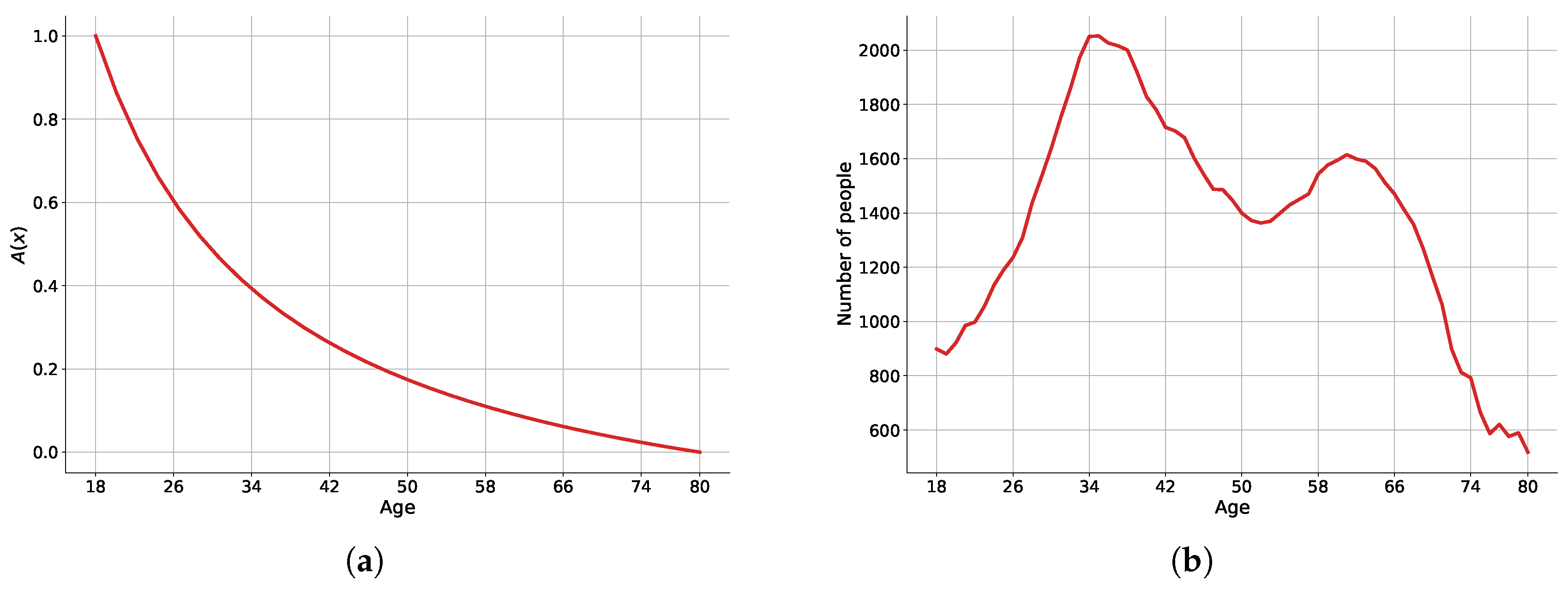
Figure 2a shows the function $g\left(x\right)$ with $a_m=18, a_M=80$. The form of the function corresponds to the idea that younger people have more opportunities to migrate, for example, for educational purposes. Middle-aged people also have some opportunities to migrate for job-related reasons, and finally, people over the age of 60 have the least opportunity to migrate.

Figure 2b shows the age distribution in the whole region averaged by years in the Leningrad region, Russia (see data source in Section 6). We noted two picks; the first relates to people around 34, and the other around 60. The corresponding function g will be equal to $g\left(34\right)=0.39$ and $g\left(60\right)=0.09$.

The function $A\left(u\right)$ is defined by computing the function $g\left(x_u\right)$, where $x_u$ is the average age in the settlement $u\in I$, averaged by time $t\in T$. It is possible to consider alternative function g, depending on other assumptions or empirical data.

The distance function: To define the distance between two locations, we must choose a subjective factor. In the context of this model, we are only concerned with the distance between locations, not the specific paths of population movement. For individuals, this can be expressed as follows: if the distance involved is significant, such as migration to the opposite side of a country, there is likely to be a difference in living conditions, and it will be more difficult to relocate, as items will need to be transported. Additionally, it can be more difficult to communicate with family members. A greater distance may represent migration to another country, where living conditions will be even more distinct and unfamiliar for the economic agent, and therefore, such migrations are less likely to occur.

The roads themselves are not strictly straight, and even aircraft do not typically follow geodesic paths. However, for the purposes of this study, we have chosen to measure distance on a sphere, as this reflects the subjective perception of distance and is more easily interpretable.

Any coordinate pair on the Earth can be expressed in terms of latitude and longitude. Using latitude and longitude, we can compute the distance between two points on a sphere by the haversine formula [53]. If the central angle is equal to $\theta$, then distance $\rho$ is equal to the product of $\theta$ and r, where r is the radius of a sphere. The haversine function is $\mathrm{hav}\left(\theta \right)={\displaystyle \frac{1-cos\theta }{2}}$.

From here, $\rho =r{\mathrm{hav}}^{-1}\left(\mathrm{hav}\left(\theta \right)\right)$. In other words, $\rho$ is equal to $2rarcsin\left(\sqrt{\mathrm{hav}\left(\theta \right)}\right)$. In our computations, r is the Earth’s radius (≈6371 km). Finally, the distance function $\rho (u,v)$ is equal to

$$\rho (u,v)=2rarcsin\left(\sqrt{{sin}^2\left({\displaystyle \frac{v_{lat}-u_{lat}}{2}}\right)+cos\left(u_{lat}\right)cos\left(v_{lat}\right){sin}^2\left({\displaystyle \frac{v_{lon}-u_{lon}}{2}}\right)}\right),$$

(4)

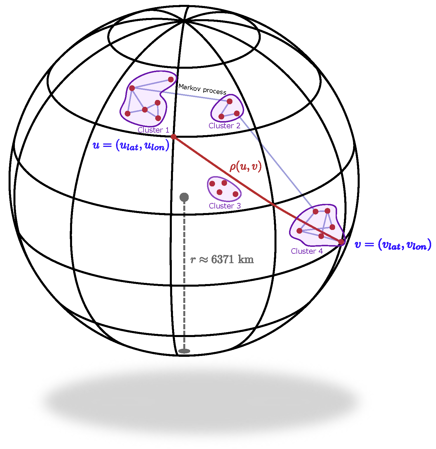
where $v_{lat}, v_{lon}$ are the latitude and longitude of the settlement $v\in I$ in radians and the same for $u\in I$, respectively. The visualization of the distance between two settlements on the Earth is represented in Figure 3.

We note that there are some clusters where settlements are located in close proximity to each other. In these clusters, people are free to move between settlements in each cluster. The interest of individuals lies in the settlements within other clusters, as these may provide different living conditions. If these conditions are superior, individuals may migrate to them. However, in order to relocate to another area, individuals need to make an effort, which may be influenced by various factors, e.g., economic or physical. Therefore, it is more challenging to travel long distances. There exists a good mathematical analogy. Let us start the stochastic process $X_t$ from the Markov family on the graph, e.g., random walk. The nodes correspond to the settlements $u\in I$ (red point in Figure 3), and the edges correspond to the roads between them (purple lines). For simplicity, the roads are represented by straight lines. Let

$$p(u,v)=P\{X_{t+1}=v|X_t=u\}$$

(5)

be the probability to move from the state u at time moment t to the state v at time $t+1$. We should choose the probabilities according to the distance between settlements. That is, we need the row-stochastic transition matrix with the size $N\times N$. Thus the process $X_t$ will spend more time in clusters and with a low probability to move to distant vertices of the graph (Figure 3).

If not every pair of nodes has roads, the transition probabilities could be determined based on the degree of the node, $p(u,v)={\displaystyle \frac{1}{d\left(u\right)}}$, if $(u,v)$ has the road and 0 otherwise, where d is the degree function. Further analysis is presented in Section 5.

The similarity function: There are various methods for identifying the similarity function. One of the most direct methods is to examine the correlation between the migration balances of settlements. Clusters of strong negative correlations indicate the existence of a group of locations that exhibit reverse patterns of movement. Similarly, clusters with strong positive correlations suggest the presence of other groups with similar patterns. To consider an alternative similarity function, it is sufficient to specify any symmetric function that takes values in the range $[-1,1]$.

The external forces: The external forces ${\lambda }_u\left(t\right),u\in I,t\in T$ are unknown, and we find them during the training process. This term refers to the external field that influences individuals and may cause them to migrate or remain in their current location. Various factors can act as an external field, such as economic, psychological, and political factors, and so on.

Due to the large number of factors involved (we refer to Section 6), it is not possible to explicitly include them in the model as separate terms in the potential energy (2). Nevertheless, we are aware that these factors do vary over time. Therefore, we assume that the functions ${\lambda }_u$ accurately represent those factors that change with time $t\in T$ and are specific to each location $u\in I$.

3.2.3. Equations of Motion

We will also continue with the analogy to physical systems and consider the “frictional” forces in the migration. This is consistent with the fact that, in order to migrate, individuals must always overcome forces that tend to dampen the system and bring it back to a state of equilibrium. These forces, for example, may include government regulations.

The generalized friction forces for the system with several degrees of freedom can be represented as ${\psi }_u=-{\sum }_v{\alpha }_{uv}{\dot{R}}_v$. The minus sign tells us the direction of the friction forces, i.e., they directed to the opposite direction with respect to generalized velocities.

In general, ${\alpha }_{uv}$ is not symmetric, but according to statistical physics, it can be shown that ${\alpha }_{uv}={\alpha }_{vu}$ [52,54]. Then, we can rewrite ${\displaystyle {\psi }_u=-\frac{\partial \mathsf{\Psi }}{\partial {\dot{R}}_u}}$, where

$$\mathsf{\Psi }={\displaystyle \frac{1}{2}}\sum _{u,v}{\alpha }_{uv}{\dot{R}}_u{\dot{R}}_v$$

(6)

is the quadratic form, the so-called dissipative function.

The Euler–Lagrange equation with dissipative function has the form

$${\displaystyle \frac{d}{dt}}{\displaystyle \frac{\partial L}{\partial \dot{R}}}={\displaystyle \frac{\partial L}{\partial R}}-{\displaystyle \frac{\partial \mathsf{\Psi }}{\partial \dot{R}}}.$$

(7)

Now, we are ready to define the Lagrangian of the system. In general, it is equal to

$$L=T-U(t,R)={\displaystyle \frac{1}{2}}\sum _{u,v}{m}_{uv}{\dot{R}}_u{\dot{R}}_v-U(t,R_1,\cdots ,R_N).$$

(8)

By substituting L in (7), we obtain

$$\begin{array}{cc}\hfill {\displaystyle \frac{\partial L}{\partial R_u}}& =-\sum _v{c}_r(u,v)f(u,v)R_v-\sum _v{c}_d(u,v)\rho (u,v)R_v-c_{a}A\left(u\right)+c_e{\lambda }_u\left(t\right),\hfill \\ \hfill {\displaystyle \frac{\partial L}{\partial {\dot{R}}_u}}& ={\displaystyle \frac{1}{2}}\sum _v{m}_{uv}{\dot{R}}_v,\hfill \\ \hfill {\displaystyle \frac{d}{dt}}{\displaystyle \frac{\partial L}{\partial {\dot{R}}_u}}& ={\displaystyle \frac{1}{2}}\sum _v{m}_{uv}{\ddot{R}}_v,\hfill \\ \hfill {\displaystyle \frac{\partial \mathsf{\Psi }}{\partial \dot{R}}}& ={\displaystyle \frac{1}{2}}\sum _v{\alpha }_{uv}{\dot{R}}_v.\hfill \end{array}$$

(9)

The resulting system of equations of the migration dynamic is equal to

$$\begin{array}{c}\hfill {\displaystyle \frac{1}{2}}\sum _v{m}_{uv}{\ddot{R}}_v+{\displaystyle \frac{1}{2}}\sum _v{\alpha }_{uv}{\dot{R}}_v+\sum _v{c}_r(u,v)f(u,v)R_v+\sum _v{c}_d(u,v)\rho (u,v)R_v+c_{a}A\left(u\right)=c_e{\lambda }_u\left(t\right),\end{array}$$

(10)

where $u\in \{1,\cdots ,N\}$.

In matrix representation, Equation (10) is transformed into

$$\mathfrak{M}\left(\begin{array}{c}{\ddot{R}}_1\\ ⋮\\ {\ddot{R}}_N\end{array}\right)+\mathfrak{A}\left(\begin{array}{c}{\dot{R}}_1\\ ⋮\\ {\dot{R}}_N\end{array}\right)+({\mathfrak{C}}_r\odot \mathfrak{R}+{\mathfrak{C}}_d\odot \mathfrak{D})\left(\begin{array}{c}{R}_1\\ ⋮\\ R_N\end{array}\right)+c_a\left(\begin{array}{c}A\left(1\right)\\ ⋮\\ A\left(N\right)\end{array}\right)=c_e\left(\begin{array}{c}{\lambda }_1\left(t\right)\\ ⋮\\ {\lambda }_N\left(t\right)\end{array}\right),$$

(11)

where

$$\begin{array}{cc}\hfill \mathfrak{M}& =\left(\begin{array}{ccc}{\displaystyle \frac{1}{2}}{m}_{11}& \cdots & {\displaystyle \frac{1}{2}}{m}_{1N}\\ ⋮& \ddots & ⋮\\ {\displaystyle \frac{1}{2}}{m}_{N1}& \cdots & {\displaystyle \frac{1}{2}}{m}_{NN}\end{array}\right),\mathfrak{A}=\left(\begin{array}{ccc}{\displaystyle \frac{1}{2}}{\alpha }_{11}& \cdots & {\displaystyle \frac{1}{2}}{\alpha }_{1N}\\ ⋮& \ddots & ⋮\\ {\displaystyle \frac{1}{2}}{\alpha }_{N1}& \cdots & {\displaystyle \frac{1}{2}}{\alpha }_{NN}\end{array}\right),\hfill \end{array}$$

(12)

$$\begin{array}{cc}\hfill {\mathfrak{C}}_r& =\left(\begin{array}{ccc}{c}_r(1,1)& \cdots & c_r(1,N)\\ ⋮& \ddots & ⋮\\ c_r(N,1)& \cdots & c_r(N,N)\end{array}\right),{\mathfrak{C}}_d=\left(\begin{array}{ccc}{c}_d(1,1)& \cdots & c_d(1,N)\\ ⋮& \ddots & ⋮\\ c_d(N,1)& \cdots & c_d(N,N)\end{array}\right),\hfill \end{array}$$

(13)

$$\begin{array}{cc}\hfill \mathfrak{R}& =\left(\begin{array}{ccc}f(1,1)& \cdots & f(1,N)\\ ⋮& \ddots & ⋮\\ f(N,1)& \cdots & f(N,N)\end{array}\right),\mathfrak{D}=\left(\begin{array}{ccc}\rho (1,1)& \cdots & \rho (1,N)\\ ⋮& \ddots & ⋮\\ \rho (N,1)& \cdots & \rho (N,N)\end{array}\right).\hfill \end{array}$$

(14)

The operation ⊙ means the element-wise product.

We do not know the exact formula for ${\lambda }_u\left(t\right),\forall u\in \{1,\cdots ,N\}$, and coefficients before each term. Coefficients can be found via a calibration procedure when solving the system of equations, but we use the approach of physics-informed neural networks to find the exact form of ${\lambda }_u\left(t\right)$ and all coefficients.

We assume that matrix $\mathfrak{M}$ has the diagonal form, i.e., $m_{ij}=0,\forall i\ne j$, and for the simplification, we use $m_{ii}=2,i\in \{1,\cdots ,N\}$. Thus, we have the coefficient 1 for the second derivatives ${\ddot{R}}_u,u\in I$. It is possible because if the matrix $\mathfrak{M}$ is invertible we can multiply by its inverse all terms in the Equation (11). Since we will be calibrating the coefficients based on the data, we can assume that they have already been multiplied by this factor in order to simplify the equations.

Finally, the system of equations of motion is defined as

$$\left(\begin{array}{c}{\ddot{R}}_1\\ ⋮\\ {\ddot{R}}_N\end{array}\right)=c_e\left(\begin{array}{c}{\lambda }_1\left(t\right)\\ ⋮\\ {\lambda }_N\left(t\right)\end{array}\right)-\mathfrak{A}\left(\begin{array}{c}{\dot{R}}_1\\ ⋮\\ {\dot{R}}_N\end{array}\right)-({\mathfrak{C}}_r\odot \mathfrak{R}+{\mathfrak{C}}_d\odot \mathfrak{D})\left(\begin{array}{c}{R}_1\\ ⋮\\ R_N\end{array}\right)-c_a\left(\begin{array}{c}A\left(1\right)\\ ⋮\\ A\left(N\right)\end{array}\right).$$

(15)

4. Lagrangian-Based Migration Model Using PINN

We employ the concept of Physics-Informed Neural Networks (PINNs) not only to solve equations of motion but also to identify unknown parameters. In our framework, we are unaware of the coefficients and the external forces that influence the migration balance dynamics. The precise formulation, often referred to as the inverse PINNs [55], merges the two model formulations: the data-driven approach and physics-based modeling (or symbolic).

Physics can be incorporated in several ways [56]. We incorporate physics into the loss function of our neural network training process. Our total loss for each training loop and for each settlement $u\in I$ is equal to

$$\mathcal{L}={\mathcal{L}}_0+{\mathcal{L}}_d+{\mathcal{L}}_p.$$

(16)

The component ${\mathcal{L}}_0$ corresponds to the initial condition. In our case, at time moment $t=t_0$, the migration balance value equals $R_u\left(t_0\right)=0$. We also constrain the velocity at the initial time point $t_0$ as ${\dot{R}}_u\left(t_0\right)=0$ (17). We choose zero values for the general framework because we subtract the first value to achieve the zero start point, and we normalize the R’s values into the range $[-1,1]$. The schematic loss evaluation is presented in Figure 4.

$${\mathcal{L}}_0=|R_u\left(t_0\right)-{\widehat{R}}_u\left(t_0\right)|+|{\dot{R}}_u\left(t_0\right)-{\displaystyle \frac{d{\widehat{R}}_u}{dt}}{|}_{t=t_0}|,$$

(17)

where $\widehat{R}$ is the approximated value of the migration balance achieved by the neural network F (Figure 4). The derivative ${\displaystyle \frac{d{\widehat{R}}_u}{dt}}$ is computed using the automatic differentiation method.

The data loss ${\mathcal{L}}_d$ is equal to the difference between the real values of the migration balance $R_u$ and the estimated balance ${\widehat{R}}_u$ from our dynamic model (18). Points that correspond to the data are denoted as $t_d$, and they are normalized into the range $[0,1]$.

$${\mathcal{L}}_d={\displaystyle \frac{1}{n_d}}{\parallel R_u\left(t_d\right)-{\widehat{R}}_u\left(t_d\right)\parallel }_2^2,$$

(18)

where $n_d$ is the number of data points.

The last loss component is the physics loss that consists of the components of Equation (10). $C_{rd}(u,v)$ and $C_{\alpha }(u,v)$ are the short notations for the corresponding terms in Equation (10).

$${\mathcal{L}}_p={\displaystyle \frac{1}{n_p}}\parallel {\displaystyle \frac{d^2{\widehat{R}}_u}{d{t}^2}}{|}_{t=t_p}+\sum _{v=1}^N\left(C_{rd}(u,v){\widehat{R}}_v\left(t_p\right)+C_{\alpha }(u,v){\displaystyle \frac{d{\widehat{R}}_v}{dt}}{|}_{t=t_p}\right)+c_{a}A\left(u\right)-c_e{\lambda }_u\left(t_p\right){\parallel }_2^2,$$

(19)

where $n_p$ is the number of physics points.

The architecture of the neural network consists of two residual blocks. Each block includes three linear layers, with a ReLU activation function applied between each layer, except for the penultimate layer. Finally, the last layer does not have an activation function, as we require the output to be a real number. Between two residual blocks, we use skip-connection with layer normalization. The input and output dimensions for each network are equal to 1, and the hidden dimension of linear layers is equal to 64.

We trained the neural networks with $20,000$ epochs and the AdamW optimizer with an initial learning rate of $0.002$ and a cosine scheduler with ${\eta }_{min}=0.0002$. Additionally, we employ the gradient norm clipping technique with a maximum norm of 1. The training process is executed on a CPU environment equipped with 8 GB of RAM and an M1 chip.

This formulation of PINN enables us to solve the dynamics Equation (10), specifically determining the values of functions at data points $t_d$ and estimating the coefficients and the non-homogeneous functions ${\lambda }_u$. We use them for the subsequent experiments with scenarios through the numerical solution of a system of differential equations.

5. Transfer Operators and Invariant Density for Settlements’ Distribution

As we do not know the exact motion of people in the region, we can think about it as some stochastic process. The typical example is the random walk on a graph. Let us have a stochastic process $X_t$ on a finite state space $U=\{u_1,\cdots ,u_N\}$. Let $p(u,v)$ be the transition probability, i.e., $p(u,v)=\mathbb{P}\{X_{t+1}=v|X_t=u\}$. Such transition probability from the row-stochastic matrix $\mathcal{S}\in {\mathbb{R}}^{N\times N}$,

$${\mathcal{S}}_{i,j}=p(u_i,u_j)\forall i,j\in \{1,\cdots ,N\}$$

(20)

On a given graph $\mathfrak{G}=(U,E,\omega )$, where U is the set of nodes (e.g., settlements), $E\subset U\times U$ is the set of edges or links (e.g., roads between settlements), and $\omega :U\times U\to \mathbb{R}$ is the weight function, we can define the random walk determined by transition matrix $\mathcal{S}$. The transition probability can be defined as

$$p(u,v)={\displaystyle \frac{\omega (u,v)}{\mathsf{\Omega }\left(u\right)}},\mathrm{where}\mathsf{\Omega }\left(u\right)=\sum _{v\in U}\omega (u,v).$$

(21)

The interpretation of the $\mathsf{\Omega }\left(u\right)$ is the out-degree of the node u, which is weighted according to the function $\omega$. Let us have some nonnegative measurable function $\mu$ on an arbitrary measure space satisfying ${\sum }_{u\in U}\mu \left(u\right)=1$. Then, it is called probability density. We can define the transfer operator on this measure space: the Perron–Frobenius operator $\mathcal{P}:L^2\to L^2$, which describes the evolution of the probability density from $L^2$.

$$\begin{array}{cc}\hfill \mathcal{P}\mu \left(u\right)& =\sum _{v\in U}p(v,u)\mu \left(v\right).\hfill \end{array}$$

(22)

As we consider graph $\mathfrak{G}$, which has a finite number of elements, it can be associated with $L^2$ space by an $N\times N$ matrix representation. Exactly,

$$P={\mathcal{S}}^T.$$

(23)

A density $\pi$ is called invariant if $\mathcal{P}\pi =\pi$. In other words, the density $\pi$ is the eigenfunction of the Perron–Frobenius operator $\mathcal{P}$, which corresponds to the eigenvalue 1.

We can find the invariant density as

$$\pi \left(u\right)={\displaystyle \frac{\mathsf{\Omega }\left(u\right)}{{\displaystyle \sum _{w\in U}}\mathsf{\Omega }\left(w\right)}}.$$

(24)

This fact is proofed as follows:

$$\mathcal{P}\pi \left(u\right)={\displaystyle \sum _{v\in U}}p(v,u)\pi \left(v\right)={\displaystyle \sum _{v\in U}}{\displaystyle \frac{\omega (v,u)}{\mathsf{\Omega }\left(v\right)}}{\displaystyle \frac{\mathsf{\Omega }\left(v\right)}{{\displaystyle \sum _{w\in U}}\mathsf{\Omega }\left(w\right)}}={\displaystyle \frac{1}{{\displaystyle \sum _{w\in U}}\mathsf{\Omega }\left(w\right)}}{\displaystyle \sum _{v\in U}}\omega (u,v)=\pi \left(u\right),$$

(25)

where we need to use the symmetry $\omega (v,u)=\omega (u,v)$. This symmetry tells us about the unprioritized direction from settlement u to v and vice versa, which is true for our undirected setting.

In fact, for a directed graph, the invariant density will take the same form. To do this, it is enough to introduce a new function $h(u,v)$, such that

$${\displaystyle \sum _{u\in U}}h(u,v)={\displaystyle \sum _{v\in U}}h(u,v)=0.$$

(26)

Then, the weight function should be equal to $\breve{\omega }(u,v)=\omega (u,v)+h(u,v)$. Since,

$$\breve{\mathsf{\Omega }}\left(u\right)={\displaystyle \sum _{v\in U}}\breve{\omega }(u,v)={\displaystyle \sum _{v\in U}}\omega (u,v)+{\displaystyle \sum _{v\in U}}h(u,v)=\mathsf{\Omega }\left(u\right),$$

(27)

for all $u\in U$ and

$$\breve{p}(u,v)={\displaystyle \frac{\breve{\omega }(u,v)}{\breve{\mathsf{\Omega }}\left(u\right)}}={\displaystyle \frac{\omega (u,v)}{\mathsf{\Omega }\left(u\right)}}+{\displaystyle \frac{h(u,v)}{\mathsf{\Omega }\left(u\right)}}=p(u,v)+{\displaystyle \frac{h(u,v)}{\mathsf{\Omega }\left(u\right)}}.$$

(28)

It immediately follows that the invariant density for the Perron–Frobenius operator defined in terms of transition probabilities for a directed graph coincides with the invariant density for the operator in the undirected setting.

We can define the initial distribution of settlements in several ways. One way is to consider a uniform distribution, where the probability $\mu \left(u\right)={\displaystyle \frac{1}{N-1}},u\in \{1,\cdots ,N-1\}$, is assigned to each settlement, with N representing the total number of settlements, including the imaginary one (we do not consider the distribution with an imaginary settlement). Another way is to define probabilities based on the migration balance for a specific year or use the average migration balance for all years. That is,

$$\mu \left(u\right)={\displaystyle \frac{R_u\left(t\right)+\left|m_t\right|}{{\sum }_{v=1}^{N-1}{R}_v\left(t\right)+(N-1)\left|m_t\right|}},$$

(29)

where $m_t={\displaystyle \underset{u\in \{1,\cdots ,N-1\}}{min}}\left\{R_u\left(t\right)\right\}$ is the minimal migration balance for the year $t\in T$.

Throughout all the years,

$$\mu \left(u\right)={\displaystyle \frac{\frac{1}{\#T}{\sum }_{t=1}^{\#T}(R_u\left(t\right)+\left|m\right|)}{{\sum }_{v=1}^{N-1}\left[\frac{1}{\#T}{\sum }_{t=1}^{\#T}(R_v\left(t\right)+\left|m\right|)\right]}}={\displaystyle \frac{{\langle R_u\left(t\right)\rangle }_t+\left|m\right|}{{\sum }_{v=1}^{N-1}{\langle R_v\left(t\right)\rangle }_t+(N-1)\left|m\right|}},$$

(30)

where $m={\displaystyle \underset{\begin{array}{c}u\in \{1,\cdots ,N-1\},\\ t\in T\end{array}}{min}}\left\{R_u\left(t\right)\right\}$ is the minimal migration balance for all years, ${\langle R_u\left(t\right)\rangle }_t={\displaystyle \frac{1}{\#T}}{\sum }_{t=1}^{\#T}{R}_u\left(t\right)$ is the sample mean, and $\#T$ is the number of years in T.

An alternative approach involves employing the similarity function between settlements. The premise is that if a settlement possesses a comparable counterpart, the probability of achieving clusters with similar elements must be equivalent or closely approximated. As we use the correlation function $f(u,v)$, we obtain

$$\mu \left(u\right)={\displaystyle \frac{{\sum }_{v=1}^{N-1}\mathbb{I}\left\{\right|f(u,v)|>c\}}{{\sum }_{u=1}^{N-1}{\sum }_{v=1}^{N-1}\mathbb{I}\left\{\right|f(u,v)|>c\}}},$$

(31)

where $\mathbb{I}$ is the indicator function, and c is the threshold in the range $[-1,1]$.

Conversely, if the settlements are identical, there is no compelling reason for individuals to relocate to them. Then we can consider the indicator function of the form $\mathbb{I}\left\{\right|f(u,v)|<c\}$. It depends on the assumptions about people’s behavior.

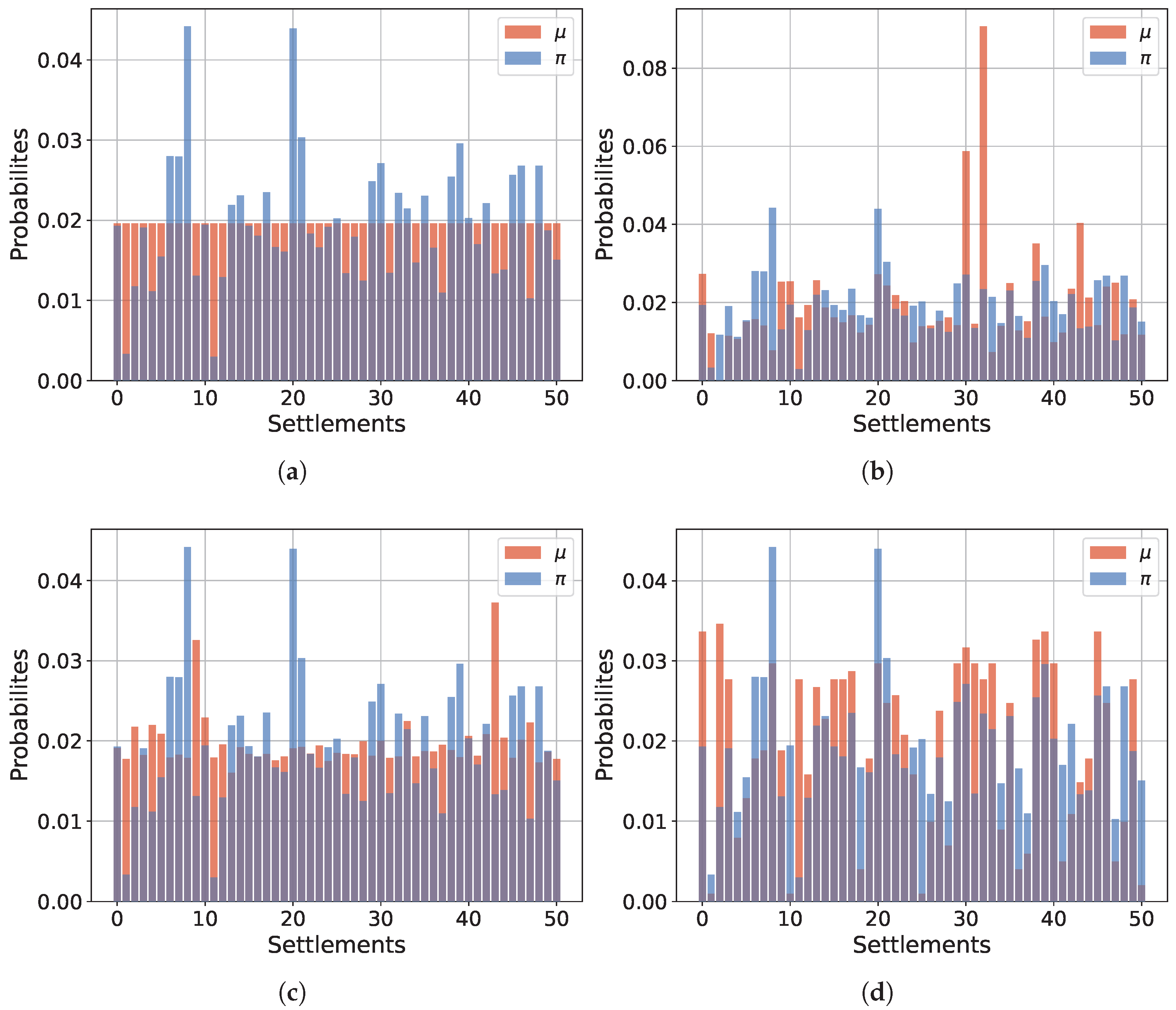
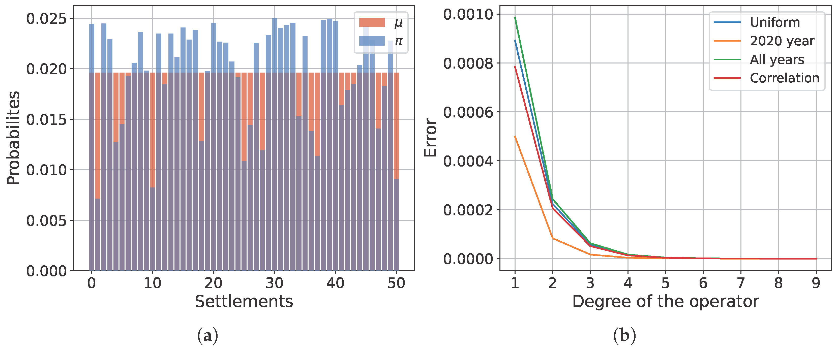
Figure 5 shows the invariant density with the weight function $\omega (u,v)$ that corresponds to the distance function $\rho (u,v)$. However, if we want that for long distances, the probability will be smaller, then we need to inverse the distance function, $\tilde{\omega }(u,v)={\displaystyle \frac{1}{\rho (u,v)}}$. In fact, since the distance between the settlement and itself is zero, it is necessary to exclude points where $u=v$ to avoid division by zero. For simplicity, in matrix notation, we can compute the matrix $\left[\tilde{\omega }\right]={\displaystyle \frac{1}{(\mathfrak{D}+E)}}-E$, where E is an identity matrix. We use the data for migration in the United States (for data description, see Section 6).

Finally, the Perron–Frobenius operator matrix is equal to ${\left[P\right]}_{u,v}={\left[S\right]}_{v,u}={\left[S\right]}_{u,v}^T$, where ${\left[S\right]}_{u,v}={\displaystyle \frac{\tilde{\omega }(u,v)}{{\sum }_v\tilde{\omega }(u,v)}}$ and the invariant density is

$$\pi \left(u\right)={\displaystyle \frac{{\displaystyle \sum _v}\tilde{\omega }(u,v)}{{\displaystyle \sum _w}{\displaystyle \sum _v}\tilde{\omega }(w,v)}}.$$

(32)

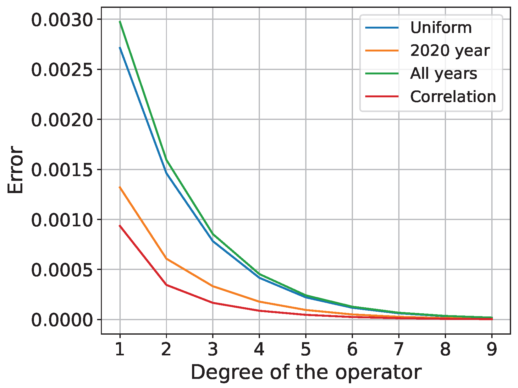
In all cases, the invariant density can be attained by applying the Perron–Frobenius operator. Each iteration of the evolutionary operator shifts the density towards the invariant density. The degree of convergence is achieved by applying a specific degree of the operator. That is, ${\mathcal{P}}^k={\displaystyle \underset{k}{\underbrace{\mathcal{P}\circ \cdots \circ \mathcal{P}}}}$.

After applying the Perron–Frobenius operator, we can obtain the new probabilities that represent the most and least prioritized settlements. Utilizing the transition matrix derived from the distances, we can deduce that for the most distant settlements, the probability of transitioning to them is lower compared with central settlements. In this case, it corresponds to the two settlements: Alaska and Hawaii.

Figure 6 illustrates the discrepancies between the evolutionary density and the invariant density for all instances of the initial probability mass function. It is evident that the most rapid convergence is attained when the initial probability mass function is derived from the migration balance in the year 2020 and from the correlations between settlements.

Another way to define the weight function is based on the correlations between settlements. For example, we define it as follows

$$\left[\widehat{\omega }\right]=\left|\mathfrak{R}\right|-E,$$

(33)

where E is the identity matrix. That is, $\widehat{\omega }(u,v)=\left|f(u,v)\right|$ for any $u\ne v$ and $\widehat{\omega }(u,v)=0$ for any $u=v$.

Figure 7 shows the invariant density with a new transition matrix based on $\left[\widehat{\omega }\right]$.

It is noteworthy that the distribution gradually differentiated not only two distant settlements but also several others that exhibited similar patterns in terms of the correlation between migration balances across all migration years.

6. Results

6.1. Data Description

We evaluate our results in three experiments. For the first experiment, we analyzed migration data within the Leningrad region in Russia, focusing on localities such as villages and district centers (https://rosstat.gov.ru, accessed on 15 January 2025). In the second experiment, we utilized data on migration patterns between regions within Russia. We considered both central and remote regions. The data for these experiments were collected and aggregated from various sources. We used the official data source, Rosstat (https://rosstat.gov.ru, accessed on 15 January 2025), and open access information (https://old.citylifeindex.ru/database?pageType=CITIES, accessed on 15 January 2025).

The third experiment involves data on migration between states in the United States of America. For this purpose, we have utilized official resources such as the Bureau of Economic Analysis by the U.S. Department of Commerce (https://www.bea.gov, accessed on 15 January 2025), the National Center of Educational Statistics (https://nces.ed.gov/programs/digest/current_tables.asp, accessed on 15 January 2025, and the U.S. Census Bureau (https://www.census.gov/data, accessed on 15 January 2025).

We selected these data because they provide a comprehensive source of information on the macroeconomic and social indicators of the territories during the specified migration years. Another significant consideration was the availability of the data, as well as their disaggregation by regions, states, etc.

After collecting the data, they were preprocessed. Firstly, for each settlement, the first value was subtracted, and then the migration balance was normalized to the range between $-1$ and 1. As a result, our data for each settlement begin at exactly zero and do not exceed one.

For the interpretation experiments, we use external factors that have been aggregated from the previously described sources. These external factors have been normalized by the population size. Our model also includes the coordinates of regional and settlement areas. For this purpose, we use publicly available data on latitudes and longitudes.

6.2. Dynamic Equation Solution

In the first experiment, we trained the PINN model and attempted to find the optimal approximation for the migration balance dynamics. We also analyzed the general patterns of behavior in the non-homogeneous function $\lambda$ according to the dynamics of the migration balance $R\left(t\right)$. Here we use the one region, the Leningrad region (Russia), and settlements within it. The number of settlements is equal to 10. We also added the imaginary city according to our methodology.

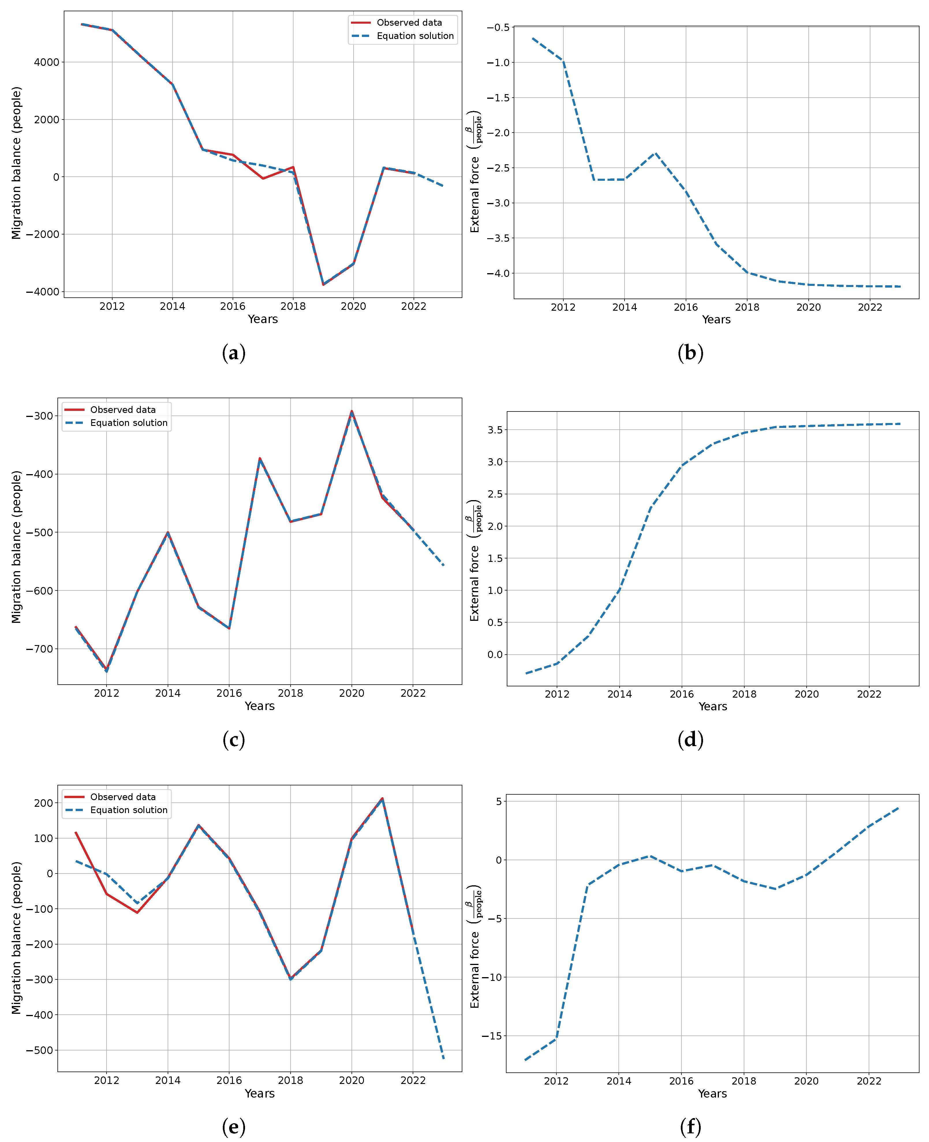
Figure 8 shows the solutions of the system of Equations (10) for the experiments with ten settlements. The right columns correspond to the non-homogeneous functions $\lambda$ (external forces) for the certain settlements. Analyzing these functions, we can understand the external influence on the migration balance dynamics.

Starting in 2014, there was an upward trend in ${\lambda }_0$, which began to influence $R_0$. In 2015, $R_0$’s downward trend reversed to an upward one, and after ${\lambda }_0$ stabilized around −36, $R_0$ increased, and then ${\lambda }_0$ increased again, causing the downward trend of $R_0$ to decrease. However, since 2018, ${\lambda }_0$ has remained around −27, and $R_0$ has been increasing. That is, when ${\lambda }_0$ remains constant, $R_0$ increases.

For settlement number 4, we can consider another scenario. The trend of $R_4$ is similar to that of ${\lambda }_4$, and the desired outcome can be achieved through the corresponding external influence.

In settlement 7, the turning point in the migration balance occurred in 2019. In this year we can also note the drop in the external migration function from 0 to $-150$. Finding such turning points in the external migration can help to analyze the corresponding settlement migration balance dynamic.

6.3. Interpretation

In our next experiments, we looked for not only to a solution but also to interpret the behavior of the non-homogeneous function $\lambda$. We considered not just a single region, but several regions, and for each region, we determined the regional center which uniquely determined by its longitude and latitude. For the second experiment, we selected 16 regions in Russia, which corresponded to 16 settlements, and we also added an imaginary city to create a conservative system. Figure 9 shows the solutions and non-homogeneous functions for this experiment.

The migration balance is dependent on the regional development and corresponding investment in that region. In the study [5], attributes were identified that allow for predicting the migration balance with a high level of accuracy. We utilize the following attributes which are available for our settlements: the average number of employers in organizations (thnd. ppl.), the average salary per month (rub.), the area of shops (thnd. sq.m.), the number of seats in restaurants, the food services turnover (mln. rub.), the commissioning of residential buildings (thnd. sq.m.), the number of sports venue, the investments per capita (mln. rub.), the number of hospitals and the number of preschool institutions. All attributes were normalized based on the population size, as the regional centers have different types of development in different parts of the country.

The functions ${\lambda }_u\left(t\right),u\in \{1,\cdots ,N\}$ are obtained by training the PINN model, where we initially only have information about each settlement u. During training, we solve Equation (10) and subsequently find the optimal right-hand side (non-homogeneous function $\lambda$) of the dynamic Equation (10). Therefore, we used attributes that describe the macro- and microeconomic situation in a given settlement and then attempted to approximate the resulting $\lambda$ using this set of features.

The simple approximation is obtained by linear regression,

$${\lambda }_u\left(t\right)=\sum _{i=1}^K{c}_i{\psi }_i(t,u),$$

(34)

where $c_i$ are coefficients and ${\psi }_i(t,u)$ are the feature functions at time moment t for each settlement $u\in I$. However, after conducting several experiments, we did not achieve the desired level of accuracy by $R^2$. Therefore, we decided to utilize a nonlinear model, such as decision trees, to improve our results.

Finally, for the model, we use XGBoost regression. In addition, we utilize the Bayesian hyperparameter optimization tool Optuna to determine the number of estimators and tree depth. Thus, we obtain 250 estimators and a maximum depth of a tree of 2. The dataset is composed of a set of described attributes, where we have interpolated their values for physical points $t_p$ with the PCHIP 1-D monotonic cubic interpolator. For the predictive variable, we use the values of $\lambda \left(t_p\right)$. Finally, we train the XGBoost model and compute on the test set the regression metrics.

To ensure statistical significance, we randomly shuffle the data and divide them into training and testing sets in an 8:2 ratio. We repeat this procedure 200 times and average the metric values.

Table 1. The quantitative results of the dynamic model evaluation. The statistically significant metrics for the reconstruction and prediction. A total of 200 experiments were conducted, and the results were averaged. Statistical significance is provided as well.

	Reconstruction Metrics		Prediction Metrics
Number of Settlements	${\mathbf{R}}^{\mathbf{2}}\pm$STD	$\mathbf{RMSE}\pm$STD	${\mathbf{R}}^{\mathbf{2}}\pm$STD	$\mathbf{RMSE}\pm$STD
16 (Russia)	$0.99\pm 1·{10}^{-4}$	$0.03\pm 2·{10}^{-3}$	$0.92\pm 0.07$	$0.24\pm 0.11$
51 (United States)	$0.97\pm 2·{10}^{-3}$	$0.01\pm 6·{10}^{-4}$	$0.91\pm 0.01$	$0.03\pm 2·{10}^{-3}$

shows the metric values, $R^2$, and root mean squared error (indicates the error in ${\displaystyle \frac{\beta }{\mathrm{people}}}$ units). Table 1 includes the reconstruction error and prediction metrics, along with their standard deviations.

The findings suggest ($R^2>0.9$) that the use of these sets of external attributes can adequately explain the non-homogeneity in Equation (10). This implies that certain factors may vary and influence this function and, consequently, migration balance.

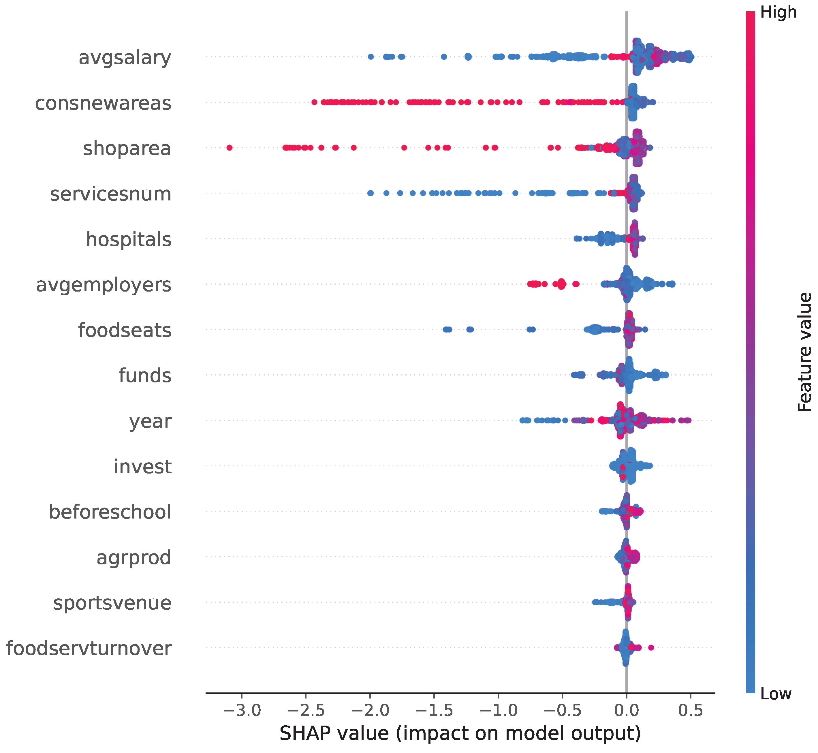
Figure 10 shows the feature importance with SHAP values. It should be noted that the average salary appears to be the most significant factor in predicting the heterogeneity functions ${\lambda }_u\left(t\right)$. At lower values, it provides an incentive to reduce the functions ${\lambda }_u\left(t\right)$ value. Furthermore, the impact of the commissioning of residential buildings and the expansion of the shop area is clearly visible. This relationship is natural, as with an increase in population in regions, local governments seek to construct homes and open additional stores. Accordingly, these factors will have a significant impact as an external force affecting migration. The absolute values of the factors are difficult to analyze, as they contribute to heterogeneity, and it is difficult to determine precisely how they will affect the migration balance.

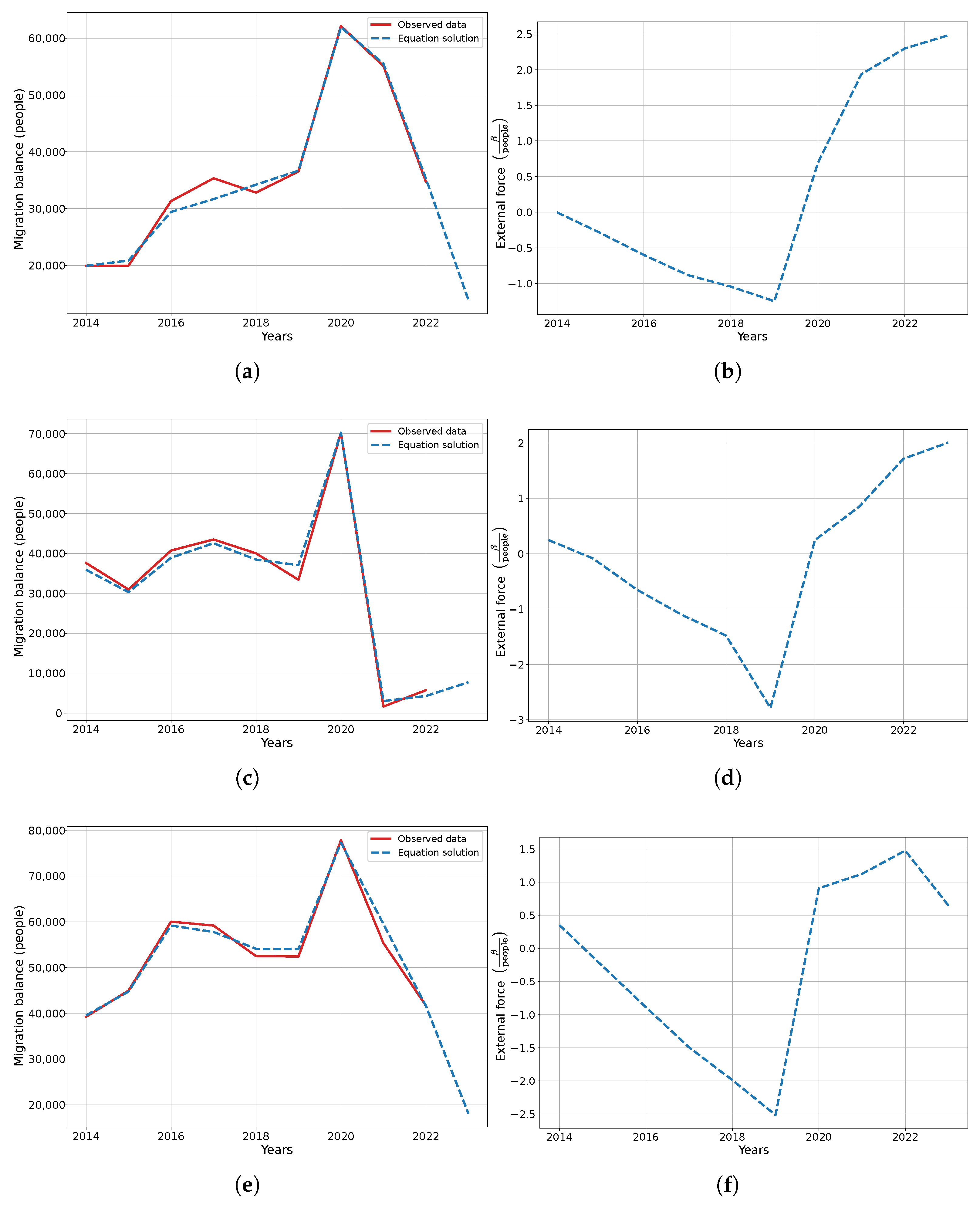
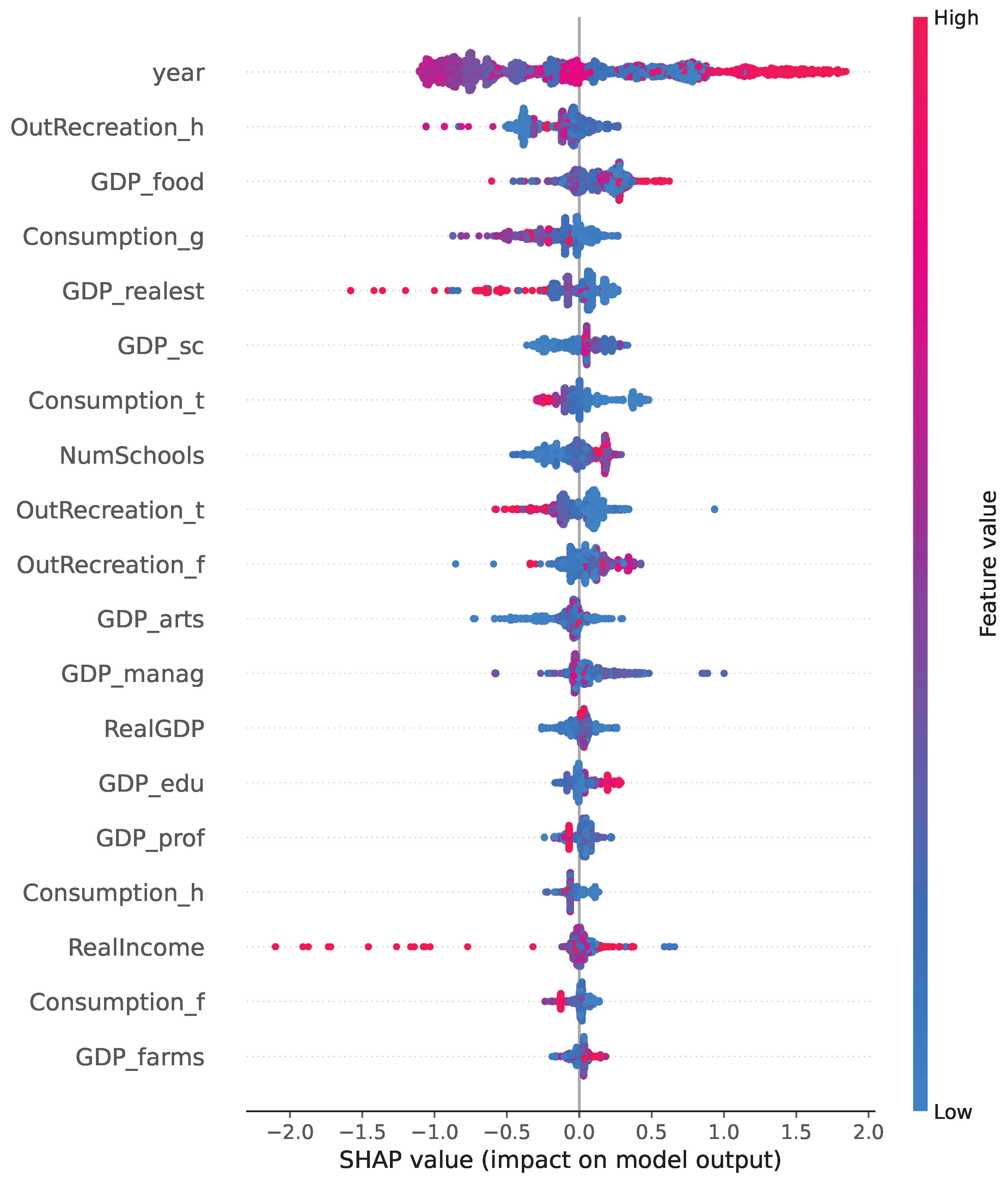
The third experiment involved internal migration within the United States. External factors may differ across countries due to variations in the level of data collection, processing, and identification of the most significant factors. Due to the fact that our experiments involved data from various countries, it was not possible to obtain a single well-aggregated dataset. Instead, we utilized a different set of macroeconomic indicators that are available in the United States for our analysis.

Our approach is independent of specific external factors, as these are used to explain heterogeneity. If a country has unique factors influencing migration, these can be incorporated into the model. For the U.S., we use the Outdoor Recreation Satellite Account (ORSA) for educational services and health care (we use the short notation _h in Figure 11), transportation services (_t), and finance and insurance (_f). The ORSA provides an assessment of the economic activity and revenue generated from outdoor recreational activities in the United States. It also tracks the production of goods and services related to these activities by various industries and their contribution to the Gross Domestic Product (GDP). Furthermore, the account provides detailed information on employment and compensation in outdoor industries. This information is useful for understanding the economic impact of these activities on the overall economy and for planning policies and initiatives that support outdoor recreation.

We also use personal consumption in transport (_t), goods (_g), health (_h), and food (_f) industries; Gross Domestic Product in food (_f), real estate (_realest), education (_edu), science (_sc), arts (_arts), profession and business services (_prof), farms (_farms), and management (_manag) industries; real income and number of schools by states (NumSchools).

Figure 11 shows solutions and non-homogeneous functions.

Figure 12 shows the significance of the external factors in the regression model. The year under review has proven to be a significant one, as it marks a period of the highest level of migration in the United States (2020 year). Additionally, significant influence have taken place in the areas of outdoor recreation in healthcare, GDP in food and real estate production, and consumption of goods and services. The quantitative results are presented in Table 1.

6.4. Visual Interpretation

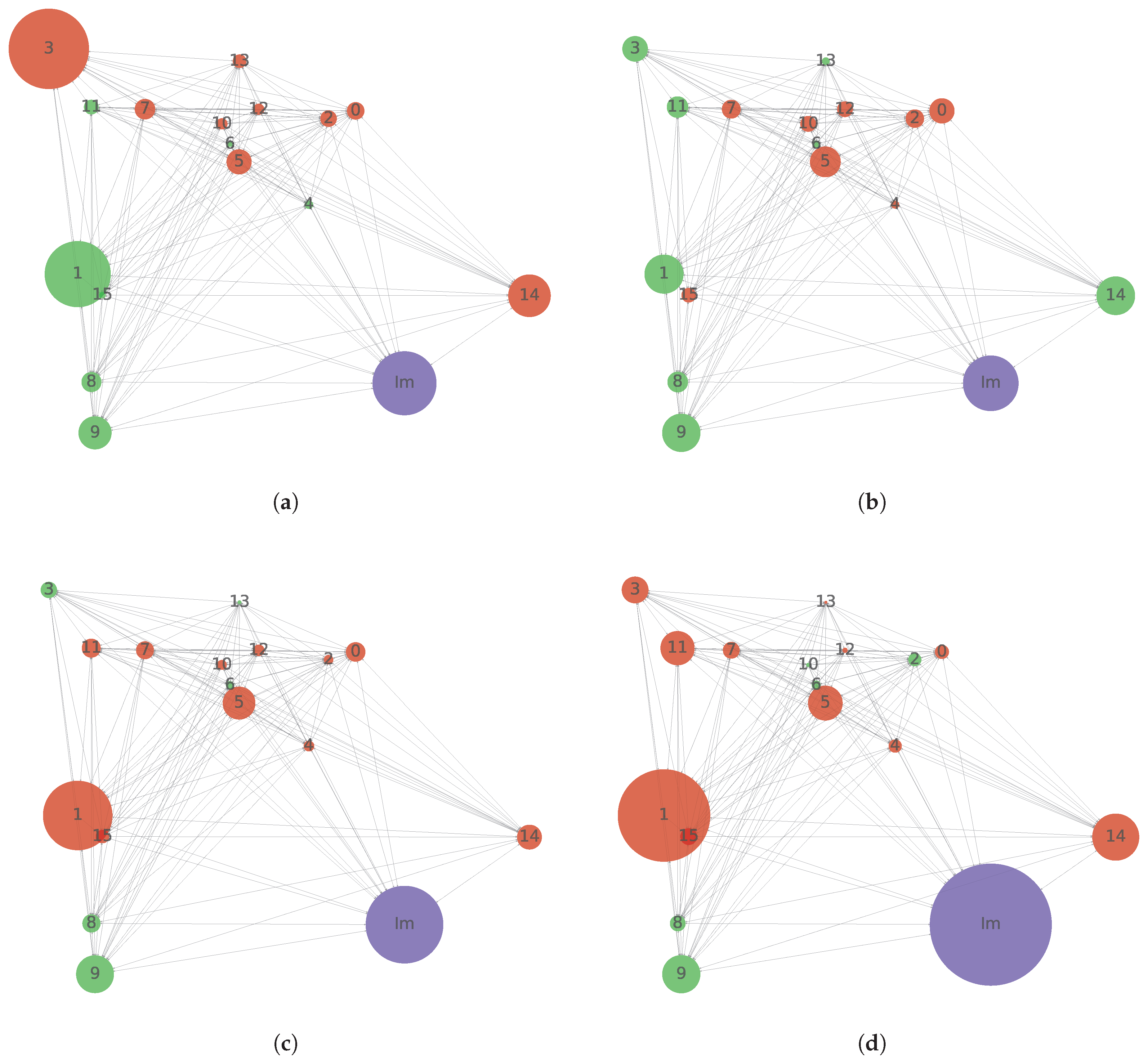
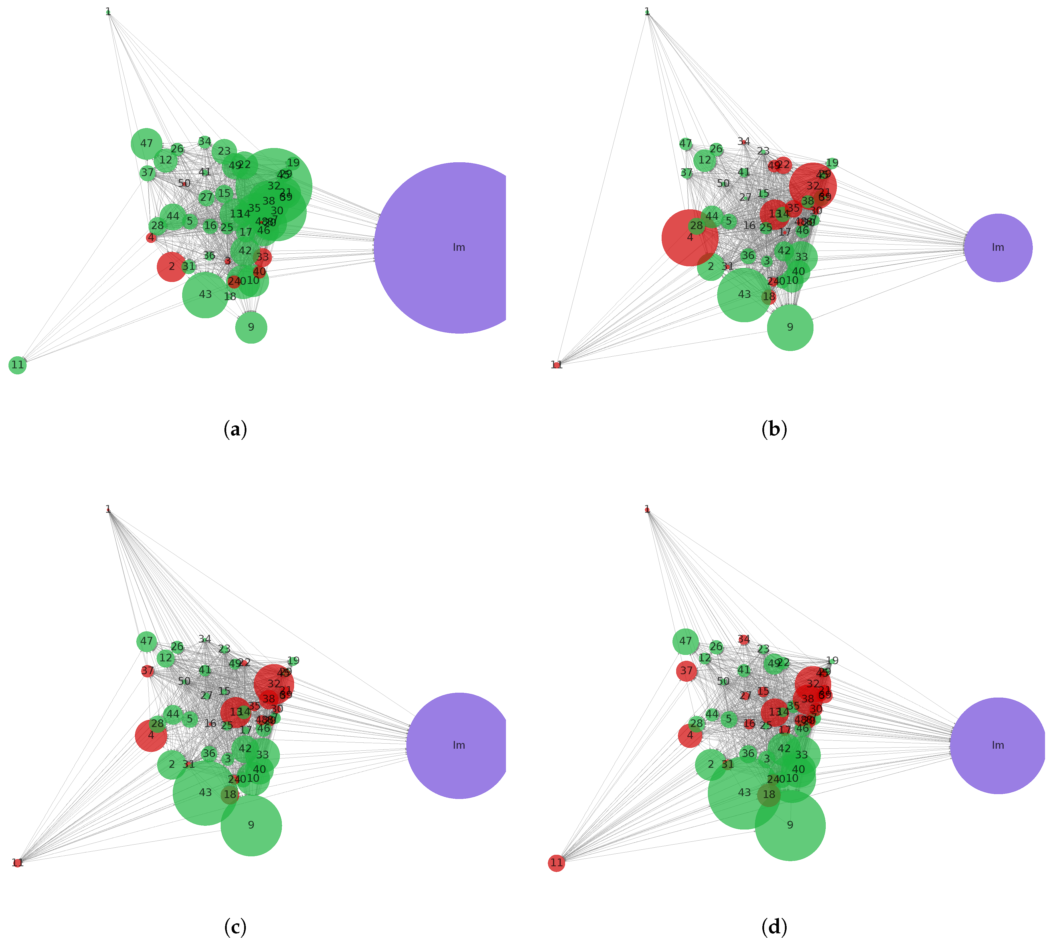
Figure 13 shows the dynamic of the migration balance in the Russian regions for the period from 2020 to 2023 years, where the data for the 2023 year are predicted by our dynamic model. The purple circle means the external migration, i.e., it is the imaginary settlement (Im), which includes the migration from and to the other region of the country or even to another country. The position of these imaginary settlements is arbitrary within the graph, as they have no specific location on a map and are simply imagined points. The size of the circle means the absolute value of the migration, i.e., the larger the circle, the greater the migration flow. We also multiplied these sizes on certain values only for visualization purposes. The green color represents the positive flow, and the red color represents the negative one.

It can be seen that a significant number of migrants come from the imaginary settlement, either within the country or from another country. The same mark indicates an outflow of people, i.e., individuals leaving from the imaginary settlement to the region’s settlements. We noted the significant outflow from the settlements with numbers $1, 3, 14$. Settlements 1 and 3 are close to the country center, while settlements 14 are too far from the central part of the country. Thus, the primary migration flows should be closer to settlements 1 and 3. However, individuals also attempt to migrate from settlements 14 to areas with more favorable living conditions.

Figure 14 shows the migration graph for the experiment with the United States. It is evident that the state with the number 11 experienced a notable outflow, characterized by its considerable distance from other states. This pattern is similar to that observed in the state with the number 1. Notably, there was a substantial surge in the number of migrants in 2020. Furthermore, the majority of these migrants are concentrated in the state with the number 32, accompanied by an additional inflow of migrants into states 9 and 43. This trend is anticipated to persist in 2023, as evidenced by the projected migration balance, which aligns with the migration news available at the time of writing the article (December 2024).

The migration graph enables us to analyze the inflow and outflow of the population. By considering the selected factors from the previous subsection, we can potentially influence the region and its neighboring areas to achieve migration targets.

7. Discussion

In this paper, we introduced a dynamic model for the identification of migration balances. Our approach is based on Lagrangian mechanics, a general framework for analyzing dynamical systems. This model assists the administrator in controlling migration processes. Administrators have the flexibility to modify the potential energy to create dynamic models with diverse characteristics that influence migration patterns. Input parameters are defined in programs (strategies) for the development of territories (regions, cities, etc.). These parameters can be modified to influence migration patterns, potentially achieving desired outcomes.

Figure 15 illustrates an experiment conducted to increase the average salary by 70% for the region with the number zero in from the second experiment on migration in the Russian regions. It is noteworthy that altering the values of the feature resulted in corresponding changes to the heterogeneity function. Subsequently, numerically solving the system of differential Equation (10) enabled us to observe alterations in the migration balance.

We may notice the low quality of the numerical method due to the neural network’s attempt to find the optimal values for the parameters of the equation, whose solution should match the given initial data. However, as we do not have exact knowledge of the heterogeneity function or the exact form of the equation, only assuming certain dependencies and taking into account randomness in training the neural network and the limited number of data points available for training (interpolation was used, but the original data were only available at certain time points), the quality of the numerical approach is not sufficient to match the original data points.

Despite the limitations of the known data, the PINN solution derived from it exhibits high accuracy in approximating the relationship. During training, the PINN was automatically differentiated into relevant terms of the equation, enabling the model to select the optimal coefficients and heterogeneity function.

For further research, it would be valuable to explore migration patterns during economic downturns. To achieve this, we require data on the correlation between macroeconomic factors and migration flows within specific regions. Additionally, in the process of constructing a dynamical system, it is possible to examine the issues of controlled variables and observe how they may influence the formation of migration patterns. These variables may include various regulations issued by local authorities and decisions made by federal and state governments. However, data are also necessary for implementing such models, which are either confidential or difficult to obtain and preprocess.

8. Conclusions

In this study, we have applied a concept from physics, Lagrangian mechanics, in order to develop a model for population migration. Specifically, we have derived a potential energy function that describes the possibility of migration based on various basic variables, including a function of distance between settlements, a function of their similarity, and age. Additionally, we have considered the influence of external factors that may affect individuals from outside the system.

To identify the non-homogeneous function and the parameters of the dynamics Equation (10), we employed PINN. Subsequently, to elucidate the external factors influencing migration patterns, we selected relevant features that impact human behavior. Therefore, we gathered data from Russia and the United States and trained a regression model. Subsequently, we analyzed the significance of the features and demonstrated the potential to construct scenarios by varying specific factors, thereby altering the function of non-homogeneity and, consequently, the migration balance.

Thus, our model is essential for comprehending the factors that influence migration and effectively managing migration within a smart city and across different regions through agglomeration.