Advancing Electric Load Forecasting: Leveraging Federated Learning for Distributed, Non-Stationary, and Discontinuous Time Series

Abstract

In line with several European directives, residents are strongly encouraged to invest in renewable power plants and flexible consumption systems, enabling them to share energy within their Renewable Energy Community at lower procurement costs. This, along with the ability for residents to switch between such communities on a daily basis, leads to dynamic portfolios, resulting in non-stationary and discontinuous electrical load time series. Given poor predictability as well as insufficient examination of such characteristics, and the critical importance of electrical load forecasting in energy management systems, we propose a novel forecasting framework using Federated Learning to leverage information from multiple distributed communities, enabling the learning of domain-invariant features. To achieve this, we initially utilize synthetic electrical load time series at district level and aggregate them to profiles of Renewable Energy Communities with dynamic portfolios. Subsequently, we develop a forecasting model that accounts for the composition of residents of a Renewable Energy Community, adapt data pre-processing in accordance with the time series process, and detail a federated learning algorithm that incorporates weight averaging and data sharing. Following the training of various experimental setups, we evaluate their effectiveness by applying different tests for white noise in the forecast error signal. The findings suggest that our proposed framework is capable of effectively forecast non-stationary as well as discontinuous time series, extract domain-invariant features, and is applicable to new, unseen data through the integration of knowledge from multiple sources.

1. Introduction

1.1. Renewable Energy Directives

The industrial revolution brought about the automation of numerous work tasks, leading to enhanced productivity and better standards of living. However, this progress came with the adverse consequence of increased ${\mathrm{CO}}_2$ emissions due to fossil fuel consumption, contributing to an increase in Earth’s temperature of over 1 K [1]. Looking ahead, Germany’s energy infrastructure may confront various issues, particularly with the shift toward decentralized power generation. Policy changes at European and national levels have dismantled electricity grid monopolies, enabling consumers to choose their own power and gas suppliers in a competitive landscape. The fifth European energy package aims to align with the Paris Climate Agreement by advocating for the expansion of renewable energy and enhancing efficiency in industries such as manufacturing, transportation, and housing [2]. Investment incentives are essential to achieve these objectives, and to this end, the Renewable Energy Directive (RED II) defines Renewable Energy Communities (REC) (Definition 1) [3]. REC participants can share and utilize self-generated heat or electrical power at lower costs. Beyond regional growth, these initiatives allow for the optimization of local energy efficiency by coupling electricity, heating, and transport sectors [4].

Definition 1

(Renewable Energy Community taken from [3]).

1.

Consists of at least 50 natural persons

2.

At least 75% of the shares are held by natural persons who are located within one postal area and a radius of 50 km

3.

No member possess more than 10% of the shares

1.2. Renewable Energy Management Systems

Regulatory and legislative developments are reshaping the dynamics of the electricity market, with emerging opportunities for district energy management systems (DEMS)—coming potentially with seventeen principal roles and an innovative IT framework in this sector [5]. Boundaries of districts are defined by either a local network transformer or a gas pressure regulator, setting them apart from neighboring districts, with each having its own unique spatial dimensions. These districts—whether located in urban, suburban, rural, or industrial settings, as well as those with mixed characteristics—have unique socio-economic and demographic features that influence their energy consumption [6,7]. Initiatives such as retrofitting buildings and modernizing heating systems can lead to lower energy consumptions. Leveraging smart demand-side management, flexible approaches in generating, consumption, and storing energy can diminish building heating demands by as much as 20% [8]. As we move towards sustainable energy supply, the orchestrated operation of buildings is gaining importance [7]. DEMS are instrumental in facilitating sector integration, minimizing electricity losses, enhancing supply reliability, and incorporating emergent technologies into the electrical grid [4]. They additionally have to control and optimize energy generation, consumption and storage resources—satisfying demands of specific balancing groups [9,10]. REC energy management systems (REC-EMS) surpass DEMS by taking on the responsibility of monitoring energy distribution and fostering synergies among various districts.

1.3. Use Case

The growing complexity of decentralized energy networks necessitates for advanced REC-EMS that facilitate automated data management across distributed systems, intelligently linking components within a REC to foster synergies and leverage flexibilities between RECs [7]. In addition to the rising use of heat pumps and electric vehicles, energy providers are obligated to provide customers with dynamic electricity pricing in accordance with EnWG (§41a) in Germany [11]. As storage systems engage with dynamic pricing, a variety of feedback mechanisms may arise, potentially resulting in electricity consumption that is sensitive to price changes [12]. To ensure the cost-effectiveness of REC-EMS, it is essential to develop REC energy consumption forecasting algorithms (REC-ECF) that are both scalable and transferable. With the energy market’s liberalization allowing prosumers freely to select their energy provider on a daily basis [13], RECs possess a dynamic portfolio of their members, as depicted in Figure 1. These members represent either particular residents of a specific REC or various elements of the energy system such as electric vehicles and heat pumps. Given that each has distinct consumption patterns, the consequent time series data tend to be non-stationary (Definition 2) and exhibit discontinuities (Definition 3). Under these circumstances, a predictive model must account for the varied member composition and be calibrated for a range of RECs. The essential objective is to uncover cross-domain as well as domain-invariant patterns within a forecasting model that can handle various time series characteristics and enhance systems with time-sensitive variations.

Definition 2

(Non-Stationarity, taken from [14]). A time series is considered stationary when its statistical characteristics remain consistent regardless of the observation time. In other words, the properties of a stationary time series do not change over time. On the contrary, if a time series exhibits trends or seasonality, it is considered non-stationary. The presence of trends or seasonality causes variations in the time series values at different points in time.

Definition 3 (Discontinuity).

Discontinuous time series possess bounds in the sequence of observations.

1.4. Contributions

There is extensive research on electrical load forecasting, with many studies claiming to outperform other algorithms. On the contrary, reviews of numerous works on this subject often conclude that they are not truly comparable due to differences in the level of aggregation, the dataset used, the forecast model applied, the data preprocessing step, the temporal resolution, and the forecast horizon. Moreover, a standard benchmark model for time series forecasting is lacking, the process behind time series is frequently under-detailed, the problem concerning model weight divergence in a non-identical and independently distributed (NON-IID) setting is only inadequatly studied, issues such as non-stationarity and discontinuity are often ignored, and significant influences of the forecast execution time on forecast results is rarely considered [15]. With respect to the explainability and interpretability of machine learning models designed for time series forecasting, there is still a deficiency [16]. Investigations into the sensitivity to input features, uncertainties tied to conditionals, and the robustness to novel scenarios are still needed when utilizing machine learning (ML) models [17]. Recent studies on time series forecasting analyze various use cases by training models with highly stochastic and distributed household data using federated learning (FL) (Definition 4). These studies primarily focus on comparing strategies for averaging model weights and clustering data, with a one-step-ahead forecast horizon, to tackle challenges associated with NON-IID data [18,19,20,21,22,23]. Given the aforementioned research gaps, we propose a time series forecasting framework that aggregates knowledge from multiple clients and is simultaneously capable of handling non-stationary, discontinuous, and NON-IID data.

Definition 4

(Federated Learning, inspired by [24,25]). Federated learning is a machine learning technique where a central model is trained across multiple devices holding local data, without exchanging it, thus preserving privacy and reducing data transfer. Local models’ updates are aggregated to improve the central model.

1.5. Organization

Following the abstract, which outlines the upcoming challenges with RECs, advocates for aggregation from multiple sources to enhance forecast quality, and provides a concise summary of this research, the introduction section describes energy management systems, the use case to be examined, the research objective, and summarizes related studies. Based on this, the structure of the paper is as follows:

• Data: The data section introduces different time series characteristics and describes the procedure of synthesizing electrical load time series of RECs, which satisfy non-stationarity and discontinuity according to the research objective.
• Methodology: Briefly describes the underlying problem and challenges concerning the research objective, and conceptualizes a framework based on certain assumptions. Subsequently, it describes the process of electrical time series (building the model input data), the time series forecast model to be evaluated, and the challenges associated with FL using NON-IID data. Lastly, various experiments are designed to extract effective learning strategies (hyper-parameterization and data sharing).
• Results: Evaluates the framework (data pre-processing, forecast model, FL setting) and determines if the forecast model is optimal.
• Discussion: Interprets the results, discusses their implications, and situates them within a broader context of the field.
• Conclusion: Summarizes the main findings and suggests directions for future research.

2. Data

To address the research objective, to conduct various experiments, to evaluate results and lastly to discuss them (Section 1.4), a huge amount of REC time series is essential, ones that encompass necessary attributes such as non-stationarity (Definition 2), discontinuity (Definition 3), stochasticity (Definition 5), autoregression (Definition 6), seasonality (Definition 7), trend (Definition 8), periodicity (Definition 9) and NON-IID on various clients. In Appendix B, Figure A2 illustrates differences between these terms, where (a), (b), (c), (d), (f) and (g) are showing non-stationary characteristics (Definition 2). For simplicity, we assume that RECs are composed of various districts (Section 1.2). Since no real dataset fulfills these requirements, we firstly generate stationary as well as distinctive district electricity consumption time series (DECTS) based on different socio-economic factors (Section 2.1). Subsequently, we use these to construct RECs with dynamic portfolios, resulting in non-stationary and discontinous time series (Section 2.2).

Definition 5 (Stochasticity).

The stochasticity of a time series refers to the inherent randomness or unpredictability in the data.

Definition 6 (Autoregression).

Autoregression is a time series modeling technique where future values are predicted based on past values of the same series.

Definition 7 (Seasonality).

Seasonality in time series is a long-term characteristic pattern that repeats at regular intervals (years).

Definition 8 (Trend).

The trend of a time series represents a long-term linear or even non-linear time-dependency in the data, typically showing sustained increase or decrease over time.

Definition 9 (Periodicity).

The periodicity of a time series refers to short-term, repetitive occurrences of specific patterns such as day of week or hour of day.

2.1. Synthesis and Analysis of Synthetic Electrical Load Time Series at District Scale

We utilize a public dataset that provides more than 5500 household electricity consumption time series with a 30-min temporal resolution, classified into 18 different ACORN groups (Definition 10), to handle the huge amount of DECTS with diverse characteristics. Since these time series are highly stochastic, we proceed as introduced in [15]: (i) Clustering ACORN household electricity consumption time series, and transforming and scaling non-Gaussian distributed data, (ii) aggregating household data to the level of districts and extracting the time series process to ensure adequate sampling of training data, (iii) training a two-step probabilistic forecasting model to ensure both seasonal and short-term variations, and (iv) iterativly generate synthetic time series. This approach is applied in conjunction with weather data (temperature, relative humidity) of central Germany for the years 2018 and 2019. It results in a total of 55 distinct ACORN subgroups, each with specific time series characteristics influenced by socio-economic factors and household size. To gain a clearer understanding of the diversity of their characteristics, we firstly calculate a correlation matrix $X_{cor}$ to obtain correlations between all ACORN subgroups. We then perform principal component analysis to reduce the dimensions to two and to illustrate it with a scatter plot (Figure 2). Since many ACORN subgroups possess similar electricity consumption characteristics, aggregating them to the level of a REC will not generate diverse time series. Therefore, we additionally apply K-means clustering with the number of clusters set to $k=10$, extracting the ten most distinctive subgroups. The effect of this filtering method is demonstrated in

Table 1. Statistics of unfiltered and filtered datasets, with respect to DECTS of various ACORN subgroups, indicating higher diversity for the filtered case.

	$\mathit{\mu }\left({\mathit{X}}_{\mathit{c}\mathit{o}\mathit{r}}\right)$	$\mathit{\sigma }\left({\mathit{X}}_{\mathit{c}\mathit{o}\mathit{r}}\right)$
Unfiltered 55 ACORN subgroups	0.88	0.08
Filtered 10 ACORN subgroups	0.82	0.12

, showing lower mean values and higher standard deviations of $X_{cor}$ for the ten most distinctive subgroups, resulting in a higher diversity.

Definition 10

(ACORN, taken from [26]). ACORN is a segmentation tool which categorizes UK’s population into demographic types.

2.2. Generate Dynamic Portfolios of Renewable Energy Communities

Besides the general definition of non-stationarity (Definition 2), there even exist more refined ones named cyclostationarity (Definition 11) [27]. Since synthetic REC time series (RECTS) should be constructed to satisfy a dynamic portfolio, they must not exhibit this characteristic. Keeping this in mind and given a set of 300 DECTS for each ACORN subgroup, we generate diverse RECTS from the ten most distintive ones (Section 2.1) in respect of certain constraints (Algorithm 1):

• No unique DECTS have to be used twice.
• Each RECTS is composed of different DECTS in varying quantities $N\in [0,7]$, depicting a time dependent residents composition vector $\overrightarrow{r_t}$ (Equation (1)) for each REC.
• Since $max\left(N\right)=7$ and only 300 DECTS exist for each ACORN subgroup, the quantity of RECTS is confined to 70.
• Each REC is assigned both a random start and a random end $\overrightarrow{r_t}$ with random various probabilities $p\in [0.1, 0.2, 0.3, 0.4, 0.5, 0.6, 0.7, 0.8]$ that $N_{i,t}$ is set to zero.
• The residents composition of REC is linearly developed using start and end $\overrightarrow{r_t}$.
• Every new day, one of ten ACORN subgroups is randomly chosen and either a new DECTS is added or an existing one is excluded, unless the linear development curve from start to end $\overrightarrow{r_t}$ is undershot or exceeded by more than 1.

$$\overrightarrow{r_t}=\left[N_{1,t},\cdots ,N_{10,t}\right]$$

(1)

where:

          $N_{i,t}:$ Quantity of specific ACORN subgroup at time t

          $i:$ Index of specific ACORN subgroup, $i\in [1,10]$

          $t:$ Index of time with a daily temporal resolution

Definition 11

(Cyclostationarity, taken from [27]). A time series may exhibit both seasonality as well as periodicity and can still remain predictable, as these cyclical patterns repeat at regular intervals. Removing these two components will strongly lead to a stationary time series.

2.3. Analyze Time Series of Renewable Energy Communities

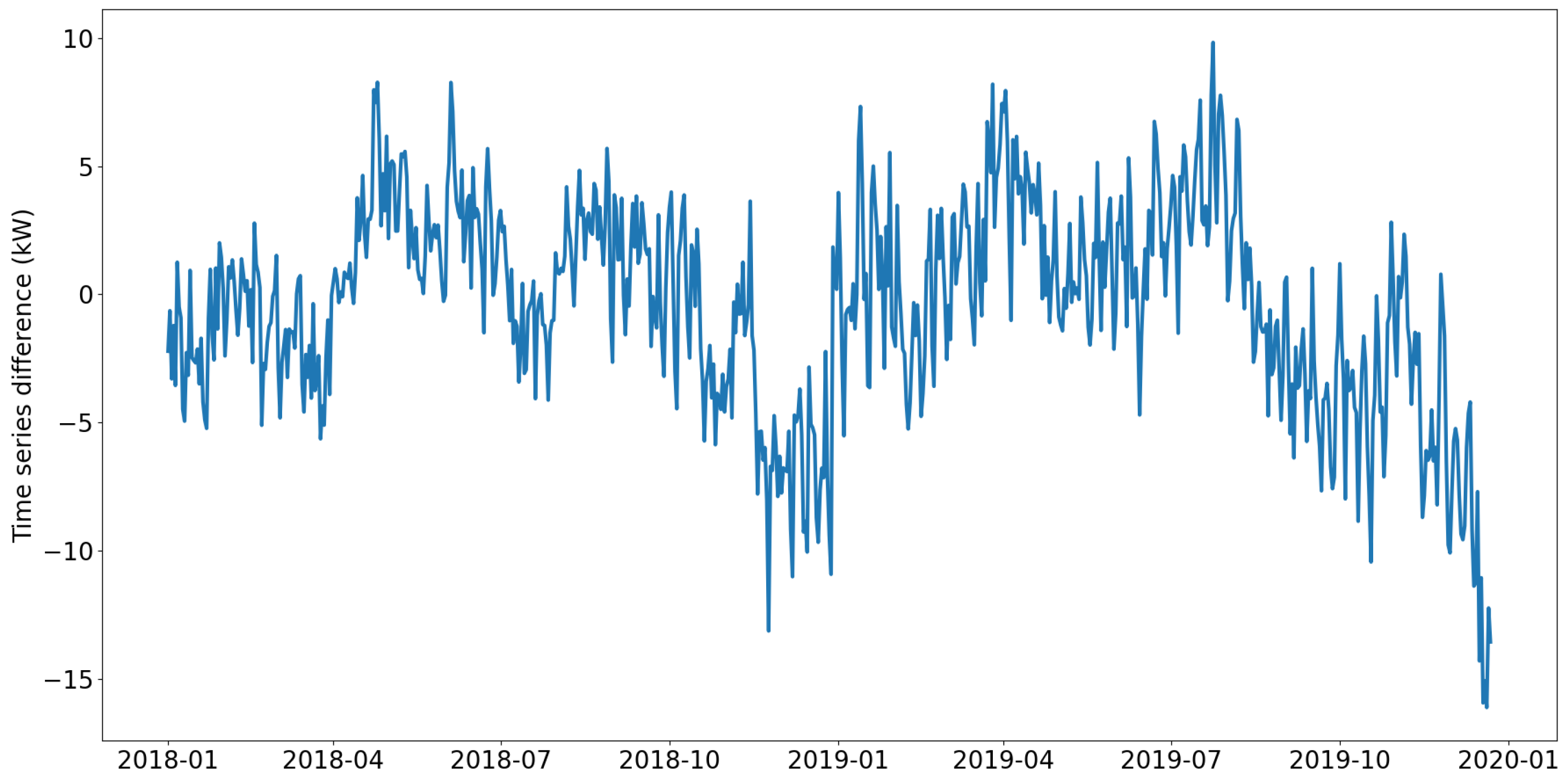
While Section 2.2 generates RECTS (examples of those can be found in Appendix A and Figure A1), we still have to test for required time series attributes. To address non-stationarity, we remove seasonality (week of the year), periodicity (day of the week, hour, minute), and even the long-term trend from the original time series by applying a Seasonal-Trend decomposition using LOESS of the Python statsmodels package. Subsequently, we apply the Augmented Dickey-Fuller (ADF) test on a representative RECTS, considering only timestamps at 12:00 (Figure 3). The Dickey-Fuller test is a statistical method for testing whether a time series is non-stationary and contains a unit root. The null hypothesis is that there is a unit root, suggesting that the time series has a stochastic trend. The ADF test considers extra lagged terms (we use $maxlag=7$ to account for an entire week) of the time series’ first difference in the test regression to account for serial correlation. Since $criticalvalue>t-valuesat1\%,5\%,10\%conficenceintervals$, the null hypothesis can not be rejected, demonstrating non-stationarity of RECTS (

Table 2. Test statistics of ADF check if RECTS is non-stationary.

Critical Value	p-Value	1%	5%	10%
−1.58	0.49	−3.44	−2.87	−2.57

, for all RECTS see Appendix D and

Table A1. Dickey fuller test statistics for all RECTS (eliminating seasonality, periodicity and trend): (i) stationary, (ii) weak non-stationary, (ii) medium non-stationary, (iv) strong non-stationary.

RECTS	Critical Value	Pvalue	1%	5%	10%
0	−2.61	0.09	−3.44	−2.87	−2.57
1	−1.83	0.37	−3.44	−2.87	−2.57
2	−2.13	0.23	−3.44	−2.87	−2.57
3	−1.93	0.32	−3.44	−2.87	−2.57
4	−2.63	0.09	−3.44	−2.87	−2.57
5	−2.75	0.07	−3.44	−2.87	−2.57
6	−2.15	0.22	−3.44	−2.87	−2.57
7	−4.01	0.0	−3.44	−2.87	−2.57
8	−3.58	0.01	−3.44	−2.87	−2.57
9	−2.71	0.07	−3.44	−2.87	−2.57
10	−3.16	0.02	−3.44	−2.87	−2.57
11	−3.83	0.0	−3.44	−2.87	−2.57
12	−3.46	0.01	−3.44	−2.87	−2.57
13	−2.18	0.21	−3.44	−2.87	−2.57
14	−1.92	0.32	−3.44	−2.87	−2.57
15	−2.51	0.11	−3.44	−2.87	−2.57
16	−2.43	0.13	−3.44	−2.87	−2.57
17	−2.39	0.14	−3.44	−2.87	−2.57
18	−2.96	0.04	−3.44	−2.87	−2.57
19	−2.78	0.06	−3.44	−2.87	−2.57
20	−2.32	0.17	−3.44	−2.87	−2.57
21	−2.11	0.24	−3.44	−2.87	−2.57
22	−2.75	0.07	−3.44	−2.87	−2.57
23	−2.94	0.04	−3.44	−2.87	−2.57
24	−2.19	0.21	−3.44	−2.87	−2.57
25	−2.08	0.25	−3.44	−2.87	−2.57
26	−2.96	0.04	−3.44	−2.87	−2.57
27	−1.91	0.33	−3.44	−2.87	−2.57
28	−2.19	0.21	−3.44	−2.87	−2.57
29	−2.04	0.27	−3.44	−2.87	−2.57
30	−1.87	0.34	−3.44	−2.87	−2.57
31	−2.11	0.24	−3.44	−2.87	−2.57
32	−3.01	0.03	−3.44	−2.87	−2.57
33	−2.48	0.12	−3.44	−2.87	−2.57
34	−1.79	0.38	−3.44	−2.87	−2.57
35	−2.09	0.25	−3.44	−2.87	−2.57
36	−1.61	0.48	−3.44	−2.87	−2.57
37	−1.77	0.39	−3.44	−2.87	−2.57
38	−1.77	0.4	−3.44	−2.87	−2.57
39	−2.15	0.23	−3.44	−2.87	−2.57
40	−1.47	0.55	−3.44	−2.87	−2.57
41	−2.11	0.24	−3.44	−2.87	−2.57
42	−1.43	0.57	−3.44	−2.87	−2.57
43	−1.87	0.34	−3.44	−2.87	−2.57
44	−1.91	0.33	−3.44	−2.87	−2.57
45	−2.01	0.28	−3.44	−2.87	−2.57
46	−2.32	0.16	−3.44	−2.87	−2.57
47	−1.77	0.4	−3.44	−2.87	−2.57
48	−1.69	0.43	−3.44	−2.87	−2.57
49	−2.42	0.14	−3.44	−2.87	−2.57
50	−2.02	0.28	−3.44	−2.87	−2.57
51	−2.7	0.07	−3.44	−2.87	−2.57
52	−2.65	0.08	−3.44	−2.87	−2.57
53	−2.41	0.14	−3.44	−2.87	−2.57
54	−1.92	0.32	−3.44	−2.87	−2.57
55	−1.63	0.47	−3.44	−2.87	−2.57
56	−1.88	0.34	−3.44	−2.87	−2.57
57	−2.35	0.16	−3.44	−2.87	−2.57
58	−2.17	0.22	−3.44	−2.87	−2.57
59	−1.88	0.34	−3.44	−2.87	−2.57
60	−0.85	0.81	−3.44	−2.87	−2.57
61	−1.61	0.48	−3.44	−2.87	−2.57
62	−2.08	0.25	−3.44	−2.87	−2.57
63	−1.87	0.35	−3.44	−2.87	−2.57
64	−1.22	0.66	−3.44	−2.87	−2.57
65	−2.13	0.23	−3.44	−2.87	−2.57
66	−2.14	0.23	−3.44	−2.87	−2.57
67	−2.2	0.2	−3.44	−2.87	−2.57
68	−2.88	0.05	−3.44	−2.87	−2.57
69	−3.49	0.01	−3.44	−2.87	−2.57

).

Algorithm 1: Generation of non-stationary and discontinous RECTS

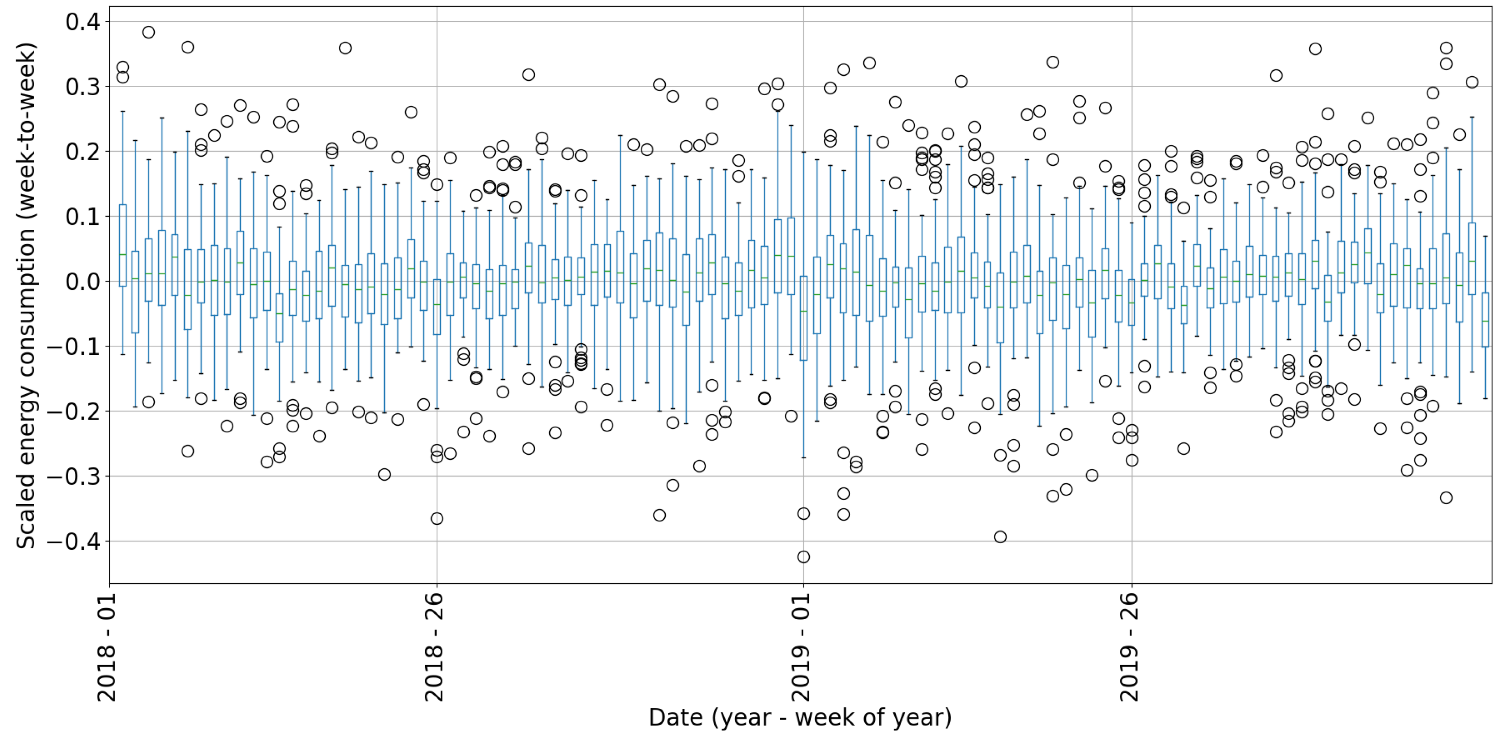
Discontinuity is often attributed to a change point, which indicates a transition from one state to another in the process generating the time series data. Various algorithms have been utilized to detect change points in data, including likelihood ratio, subspace model, probabilistic, kernal-based, graph-based and clustering methods [28]. In contrary, a boxplot is easy to use and give overview about data distribution, skewness and outliers [29]. In this, the box shows the interqurtile range (IQR) which is the distance between the first (Q1) and third (Q3) quartiles. The whiskers extend from the box to the highest and lowest values within $[Q1-1.5\times IQR,Q3+1.5\times IQR]$. The line in the middle of the box represents the median or the second quartile (Q2) of the data. Points outside the whiskers represent outliers. To analyze discontinuity in RECTS, we firstly calculate mean daily sequences for each week of the year. Subsequently, we compute differential time series (time series minus its lagged version with shift of 1). Considering that all 70 RECTS have varying magnitudes, we normalize them by utilizing Equation (2). Then, we use a boxplot to illustrate the distribution of all generated RECTS for each week of the year (Figure 4), showing a huge number of outliers and proving discontinuity in data.

$$x^{\prime }={\displaystyle \frac{x}{max\left(x\right)}}$$

(2)

Another requirement involves handling NON-IID data across multiple clients, which can be simply demonstrated by illustrating correlations among all generated RECTS. Figure 5 shows their correlation matrix $X_{rec,corr}$, with highest correlations on the diagonal—representing correlations of each RECTS to itself. Since each REC is individually developed using diverse ${\overrightarrow{r}}_t$ at start and end point, correlations are much lower than the ones of DECTS (compare Table 1 with

Table 3. Statistics of the correlation matrix $X_{rec,corr}$ for all RECTS.

$\mathit{\mu }\left({\mathit{X}}_{\mathit{r}\mathit{e}\mathit{c},\mathit{c}\mathit{o}\mathit{r}\mathit{r}}\right)$	$\mathit{\sigma }\left({\mathit{X}}_{\mathit{r}\mathit{e}\mathit{c},\mathit{c}\mathit{o}\mathit{r}\mathit{r}}\right)$
$0.51$	$0.18$

). This strongly indicates, that RECTS possess a high degree of NON-IID data, which must be adequatly considered within a time series forecasting model and FL.

2.4. Transformation

Time series data should be scaled before being used in machine learning, particularly because of algorithm performance and gradient descent optimization. In our work, we utilize Equation (3) to scale data within the range $[-1,1]$ by setting $a=-1$ and $b=1$. To rescale transformed data to its original magnitude, we use Equation (4)

$$x^{\prime }=a+{\displaystyle \frac{(x-min(x\left)\right)\times (b-a)}{max\left(x\right)-min\left(x\right)}}$$

(3)

$$x=min\left(x\right)+{\displaystyle \frac{x^{\prime }\times (max\left(x\right)-min\left(x\right))-a}{b-a}}$$

(4)

3. Methodology

3.1. Problem Description

Time series are governed by a stochastic process, meaning that both past observations $X_t$ and random shocks ${ϵ}_t$ directly influence future values $Y_{t+1}$. In terms of RECTS, the impact of autoregressive variables $X_t$ and ${ϵ}_t$ on $Y_t$ is dependent on temporal features like weekday or daytime and additionally varies from one RECTS to the next, resulting in individual forecast model parameters. The primary challenge is to create a forecast model that learns features which are consistent across different REC residents composition $\overrightarrow{r_t}$ (domains) and can be generalized to a vast array of RECs, even those not included in model training. Moreover, this forecast model should account for non-stationarity and discontinuity with regard to dynamic portfolios of RECs. Since all RECTS are assumed to be located on distributed clients, the model training process must address privacy and security concerns through the application of FL, which must manage NON-IID data and weight divergence.

3.2. Concept

Based on the problem description, we develop an approach that satisfies requirements and addresses unresolved challenges. Firstly, we provide a brief description of the time series process of RECTS by illustrating process equations. In addition to exogenous variables such as weather, we precisely incorporate the time-dependent residents composition $\overrightarrow{r_t}$ of RECs into these equations (Section 3.3). Since these process equations reflect past, present, and future states, each with potentially different $\overrightarrow{r_t}$, we take this into account during the development of the forecast model—feedforward neural network (FNN) (Section 3.4). To train across multiple distributed clients, we also develop a FL framework that offers flexibility in forecast model parameterization (such as layer type, number of neurons, batch size, and optimizer type for gradient descent) and data sharing, aiming to overcome NON-IID and model weight divergence issues (Section 3.5). Finally, we set up meaningful experiments to distinguish between ineffective and effective settings (Section 3.6). For this, we must make some assumptions:

• All RECs are composed of the same distinct DECTS, as described in Section 2.2.
• All RECs are aware of the history of their $\overrightarrow{r_t}$.
• For effective model training using FL, all RECs must share the minimum and maximum values of their RECTS to achieve consistent data scaling over all clients.

3.3. Time Series Process

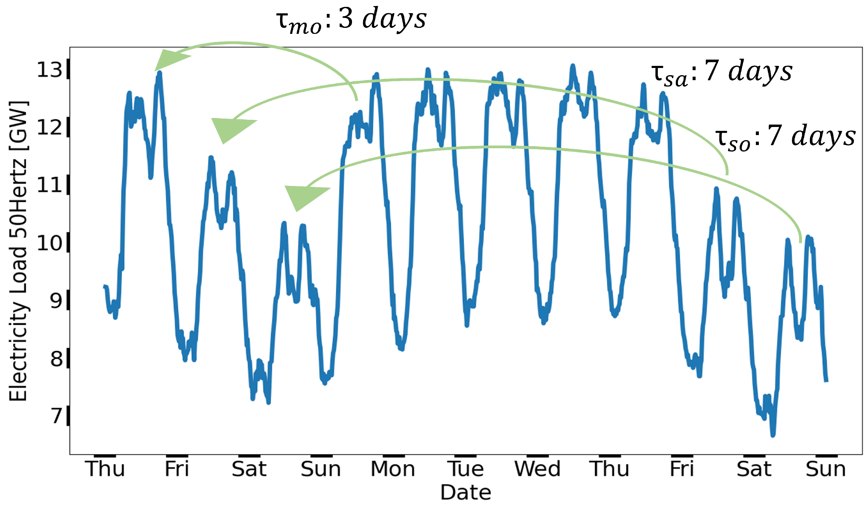
RECTS, and time series in general, are composed of seasonal (regular long-term or annual variation), periodic (regular short-term or weekday variation), trend (long-term directional movement) and irregular (white noise, which can not be modeled) components. Time series can be predicted by extrapolating from past and present observations into the future, commonly utilizing an AutoRegressive Integrated with eXogenous variables (ARIX) model. In this context, AR is associated with present observations, I is associated with past observations, and X encompasses the impact of exogenous variables across past, present, and possible future (F) events. Then, a time series forecasting model should learn relationships between all variables (endogenous and exogenous) at past, present, and future timestamps. Within this framework, exogenous further variables include data of calendar, weather, and residents composition of REC $\overrightarrow{r_t}$ (

Table 4. Description of endogenous and exogenous variables used in past (I), present (AR) and future (F) regression equations.

Data Type	Variable	Description	Considered in
target	RECTS	provide target states	AR, I
calendar	day of year (doy)	models annual seasonality	AR, I, F
calendar	day of week (dow)	models short-term periodicity	AR, I, F
calendar	daytime (dt)	models intraday periodicity	AR, I, F
weather	temperature (T)	models T dependencies	AR, I, F
weather	relative humidity (RH)	models RH dependencies	AR, I, F
residents composition	${\overrightarrow{r}}_t$	models $\overrightarrow{r_t}$ dependencies on RECTS stochasticity	AR, I, F

). In our approach, we encode calendar features using cyclical encodings (Definition 13), resulting in lower dimensions [30,31]. We determine the number of lagged values $p=2$ that have a strong impact on subsequent values by following the Box-Jenkins method and utilizing the partial autocorrelation function [32]. Since I is utilized to address short-term non-stationarities, we use reference values based on the type of day (such as day of the week, holiday, or bridge day), resulting in the following shifts $\tau$ (Figure 6):

• monday → last friday ($\tau =3days$)
• tuesday → yesterday ($\tau =1days$)
• wednesday → yesterday ($\tau =1days$)
• thursday → yesterday ($\tau =1days$)
• friday → yesterday ($\tau =1days$)
• saturday → last saturday ($\tau =7days$)
• sunday → last sunday ($\tau =7days$)
• holiday → last sunday ($\tau =xdays$)
• bridge day → last saturday ($\tau =xdays$)

With this information, we can formulate regression equations for AR (Equation (5)), I (Equation (6)), and F (Equation (7)) within the context of an ARIX model to generate input data ($X_{AR}$, $X_I$, $X_F$) for the purpose of model training purposes, while disregarding the difference filter. This subsequently yields the complete ARIX process equation (Equation (8)). Given that historical data of $\overrightarrow{r_t}$ is available for each REC and is also included in the input data, there is potential to extract cross-domain and domain-invariant features, a process known as domain adaptation [33,34,35].

Definition 12

(One-Hot Encoding, taken from [15]). Within a one-hot encoding, each class is represented by a binary vector. In this encoding, each class occurrence assigns to 1 and otherwise to 0.

Definition 13

(Cyclical Encoding, inspired by [15]). Periodic encodings are transformations of one-hot encodings into more continuous variables by using sine and cosine functions. This can only be applied to periodic variables like daytime, day of the week or day of the year.

Example: For the cyclical transformation of all hours $h\in [1,24]$, we use both sinus $sin\left({\displaystyle \frac{2\times \pi \times h}{max\left(h\right)}}\right)$ and cosine $cos\left({\displaystyle \frac{2\times \pi \times h}{max\left(h\right)}}\right)$ transformations to create two new variables.

$$X_{AR}\left(t\right)=\sum _{j=1}^n\sum _{i=1}^p\left({\alpha }_{j,i}\times x_j(t-i)\right)$$

(5)

$$X_I\left(t\right)=\sum _{j=1}^n\left({\beta }_j\times x_j(t-\tau )\right)$$

(6)

$$X_F\left(t\right)=\sum _{j=1}^n\left({\gamma }_j\times x_j\left(t\right)\right)$$

(7)

$$y\left(t\right)=X_{AR}+X_I+X_F$$

(8)

where:

p	Number of past observations to be considered in AR
$\alpha$, $\beta$, $\gamma$	Regression parameters within an ARIX model
n	Number of variables used in regression equation (Table 4)
x	variable

3.4. Time Series Forecast Model

In the context of time series forecasting, a huge amount of various neural network architectures have been studied [16,31]. While neural networks and ARIX regression models may utilize identical input data (refer to Section 3.3), neural networks do not necessitate a predefined regression equation and are adept at discovering non-linear relationships and latent characteristics. This paper posits that the accuracy of forecasts is largely influenced by the choice of input features, the engineering of features (such as calendar data), and the manner in which past, present and future features are connected within the model’s architecture. A time series forecasting model is expected to discern the linkages between past, present and present endogenous and exogenous variables (see Equations (5) and (6)) and leverage this knowledge alongside future exogenous variables (Equation (7)) to predict the target variable. To this end, we propose a neural network with distinct input layers $L{1}_I$, $L{1}_{AR}$, $L{1}_F$ processing past $X_I$, present $X_{AR}$, and future $X_F$ data, each equipped with an equivalent neuron count to facilitate feature learning. Subsequent to this, latent features are combined following a principle of action (either concatenation or multiplication), and the resulting array is then processed within an output layer $L2$, conforming to the target output dimensions (illustrated in Figure 7). This architectural design can be implemented utilizing Tensorflow Keras Dense layers (FNN). In our work, we use three input layers, each with 30 neurons, and one output layer, with each layer equipped with a linear activation function.

Figure 6. Electricity load time series of 50Hertz [36] showing exemplary temporal shifts (${\tau }_{sa}$: 7 days, ${\tau }_{so}$: 7 days, and ${\tau }_{mo}$: 3 days) used in the itegrated part I (Equation (6)).

Figure 6. Electricity load time series of 50Hertz [36] showing exemplary temporal shifts (${\tau }_{sa}$: 7 days, ${\tau }_{so}$: 7 days, and ${\tau }_{mo}$: 3 days) used in the itegrated part I (Equation (6)).

3.5. Federated Learning

FL was introduced to train a high-quality global model while keeping training data distributed across multiple clients, thereby ensuring data privacy as well as security issues, and demonstrating robustness to NON-IID data. Additionally, model performance can be improved by training a model with a diverse array of training data. To achieve this, the FederatedAveraging algorithm (Algorithm 2) applies stochastic gradient descent within local model training and averages each client’s model weights on a central server [37]. In the context of energy time series forecasting, many publications have studied the application of FL at household level. Given that this data is highly stochastic and NON-IID, they propose using a one-step-ahead forecast horizon and clustering similar clients into groups, resulting in multiple global forecast models, which are further fine-tuned by applying transfer learning [24,25,38,39,40,41]. The presence of subsequences within aggregated electrical load time series has already been identified using variational mode decomposition. When combined with federated clustering, this method generates accurate forecasts [42]. While these approaches overcome issues with NON-IID data, there is no one that attempts to unify heterogeneous time series data into a single global forecast model, addressing non-stationarity and discontinuity. The reason for doing so is that a NON-IID data setting across multiple clients can lead to a divergence in model weights (Figure 8). Moreover, the number of hidden neurons N can significantly impact model convergence because gradients tend to increase when N is low. This effect can be observed during the optimization of model weights that do not align well with local data distributions and characteristics. A common practice, among others, for addressing this effect is to share data across multiple clients, which is beneficial for aggregating knowledge of relational behavior [43] (Figure 9).

Algorithm 2: FederatedAveraging

3.6. Experiments

Our work aims to bridge the research gap in training time series forecasting models using Federated Learning, addressing non-stationarity and discontinuity, as previously mentioned in Section 1.4. For this purpose, we outline the time series process, including preprocessing of model input data (Section 3.3), develop a generic neural network architecture that handles non-stationarities, discontinuities, and domain-specific characteristics across various observation times—including past, present, and future (Section 3.4), and construct a FL framework to aggregate knowledge from a diverse set of clients by applying data sharing (Section 3.5). In our experiments, we apply various model parameterizations (

Table 5. Various forecast model parameterizations in terms of batch size, the number of shared time series to each client, and the learning rate.

Forecast Model	Batch Size $\mathit{B}\mathit{S}$	Shared Time Series $\mathit{S}\mathit{T}\mathit{S}$	Learning Rate $\mathit{L}\mathit{R}$
M1	16	0	0.0001
M1	64	0	0.0001
M2	16	2	0.0001
M3	64	2	0.0001
M4	16	0	0.001
M5	64	0	0.001
M6	16	2	0.001
M7	64	2	0.001

) that include different values for the number of shared time series to each client (STS →extract relational behavior of RECTS with various ${\overrightarrow{r}}_t$ [43]), the batch size (BS →generalize neural network [45]) and the learning rate (LR →regularize model weight divergence [44]), while maintaining a certain loss function Equation (9) with $\alpha =0.9$ accounting for bias and strong outliers, the number of hidden neurons $N=30$, local training epochs $e=1$ and FL training epochs $E=50$. While training local forecasting models with stochastic gradient descent, we use Federated Averaging (Algorithm 2) to update global model weights within the entire FL process. Training data is prepared for a subset of $C_1=35$ clients with a small member size, considering the year 2018, and it is processed for a forecast execution time of 06:00 with a horizon spanning an entire day. To demonstrate our framework’s capability concerning domain-adaption, transferability, and performance, we need to design meaningful experiments (test data is a subset of $C_2=35$ clients with large member size, considering the year 2019) that differentiate between ineffective and effective settings (

Table 6. Experiments to be conducted, evaluated, and compared to gain knowledge about effective FL settings for non-stationary, discontinous, and NON-IID RECTS.

No.	Objective	Setting
I.	Train FNN for all RECs regarding ${\overrightarrow{r}}_t$ using federated learning (multi RECTS). In this study, we use $C=35$ REC with a small member size to illustrate the model’s transferability to out-of-sample data.	share RECTS to each client $STS\in [0,2]$ use multiple batch sizes $BS\in [16,64]$ use multiple learning rates $LR\in [0.001,0.0001]$
II.	Train FNN for each REC neglecting ${\overrightarrow{r}}_t$ (single RECTS) and compare them	Use best setting of experiment I.
III.	Train FNN for each REC providing ${\overrightarrow{r}}_t$ (single RECTS) and compare them	Use best setting of experiment I.
IV.	Train a FNN for all RECs neglecting ${\overrightarrow{r}}_t$ (multi RECTS) and compare them	Use best setting of experiment I.
V.	Train a FNN for all RECs providing ${\overrightarrow{r}}_t$ (multi RECTS) and compare them	Use best setting of experiment I.

). Figure 10 illustrates the process of conducting the various experiments. In Appendix C, Figure A3 illustrates the average number of members for each REC and their overall median value $med$. Regarding this, $C_1$ refers to RECs smaller than $med$ and $C_2$ refers to RECs larger than $med$, dividing train and test dataset into two distinct subsets of time series, each with characteristic behaviors and magnitudes. We use TensorFlow [46], an open-source machine learning framework, and Stochastic Gradient Descent optimization algorithm.

$$Loss=(1-\alpha )\times \left|{\displaystyle \frac{1}{N}}\sum _{i=1}^N(y-\widehat{y})\right|+\alpha \times {\displaystyle \frac{1}{N}}\sum _{i=1}^N{(y-\widehat{y})}^2$$

(9)

Figure 9. Approaches to data sharing include: (a) not sharing any time series, (b) sharing one time series, and (c) sharing two time series.

Figure 9. Approaches to data sharing include: (a) not sharing any time series, (b) sharing one time series, and (c) sharing two time series.

4. Results

4.1. Experiment I

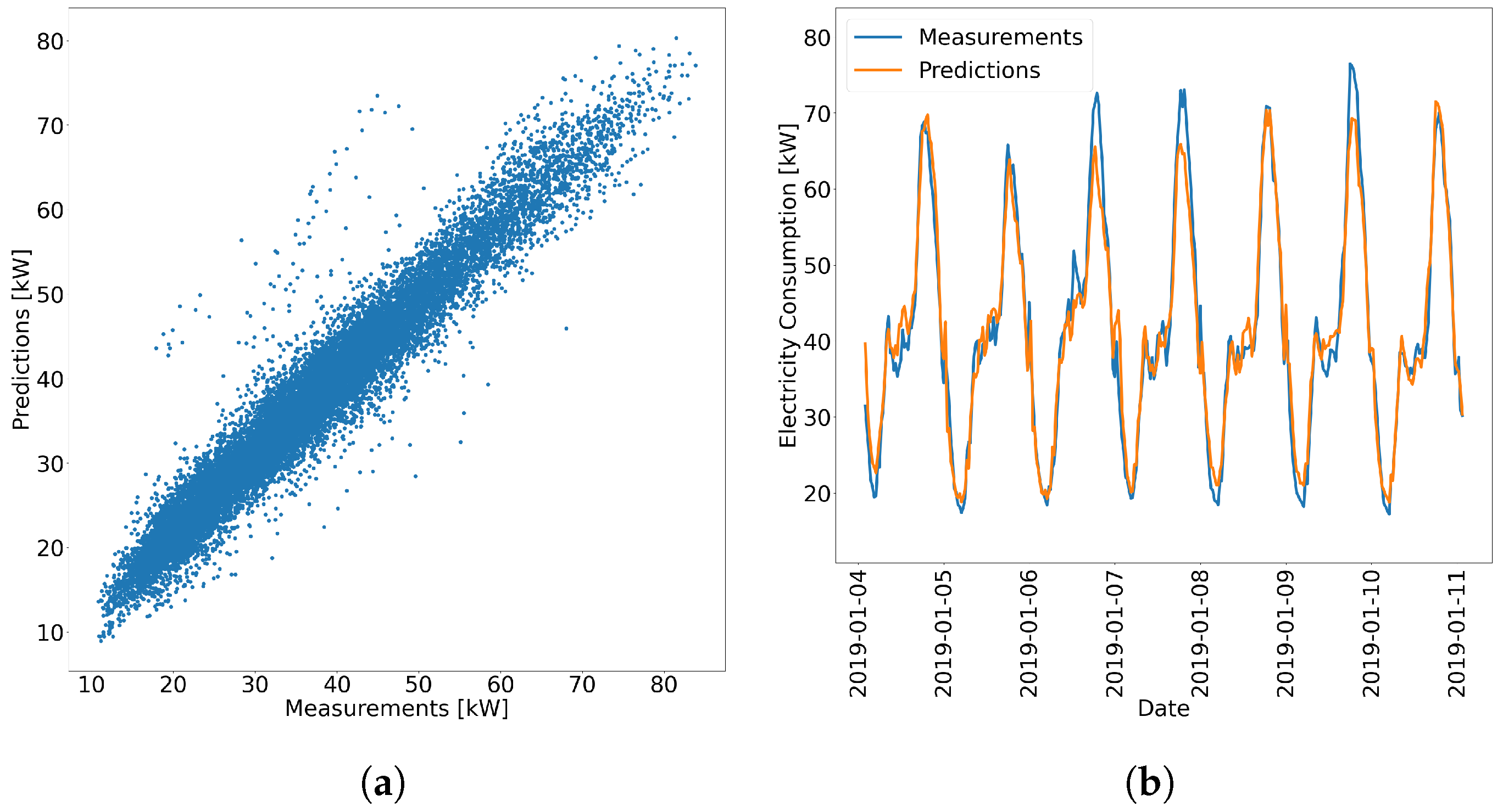
Experiment I is intended to identify the best model setting, which is then applied in subsequent experiments as well.

Table 7. MAE and MAPE from various models trained with data from clients with a small member size and tested on clients with a large member size.

	M0	M1	M2	M3	M4	M5	M6	M7
MAE [kW]	5.57	7.30	4.10	5.89	2.68	3.85	2.65	3.18
MAPE [%]	17.18	22.70	12.40	18.23	8.10	12.04	8.03	9.77

displays the mean absolute error (MAE, Equation (10)) and the mean absolute percentage error (MAPE, Equation (11)) for each model applied to the test dataset (year 2019), showing strong dependencies on batch size, learning rate, and number of shared time series. The results propose to use a smaller batch size (compare error measurements between M0 and M1, between M2 and M3, between M4 and M5, or between M6 and M7), a higher number of shared RECTS with all clients (compare error measurements between M0 and M2, between M1 and M3, between M4 and M6, or between M5 and M7), and a bigger learning rate (compare error measurements between M0 and M4, between M1 and M5, between M2 and M6, or between M3 and M7). While models with higher learning rates converge faster and yield favorable error measurements, the others struggle to learn meaningful latent features necessary for transferable predictions. Moreover, $E=50$ federated learning epochs are sufficient for the models to converge (see Figure 11). Since these error measurements do not provide a clear overview of our forecasting framework’s capabilities, we further illustrate the predictions versus actual measurements in Figure 12. The scatter plot (a) shows good agreement, except for some outliers that could possibly be caused by high variability during special events, and the line plot (b) confirms these findings. Since M6 provides best prediction results, we will use this setting within the experiments II–V.

$$MAE={\displaystyle \frac{1}{n}}\sum _{i=1}^n|y_i-{\widehat{y}}_i|$$

(10)

$$MAPE={\displaystyle \frac{1}{n}}\sum _{i=1}^n\left|{\displaystyle \frac{y_i-{\widehat{y}}_i}{y_i}}\right|$$

(11)

where $y_i$ represents measurements and ${\widehat{y}}_i$ represents forecasts.

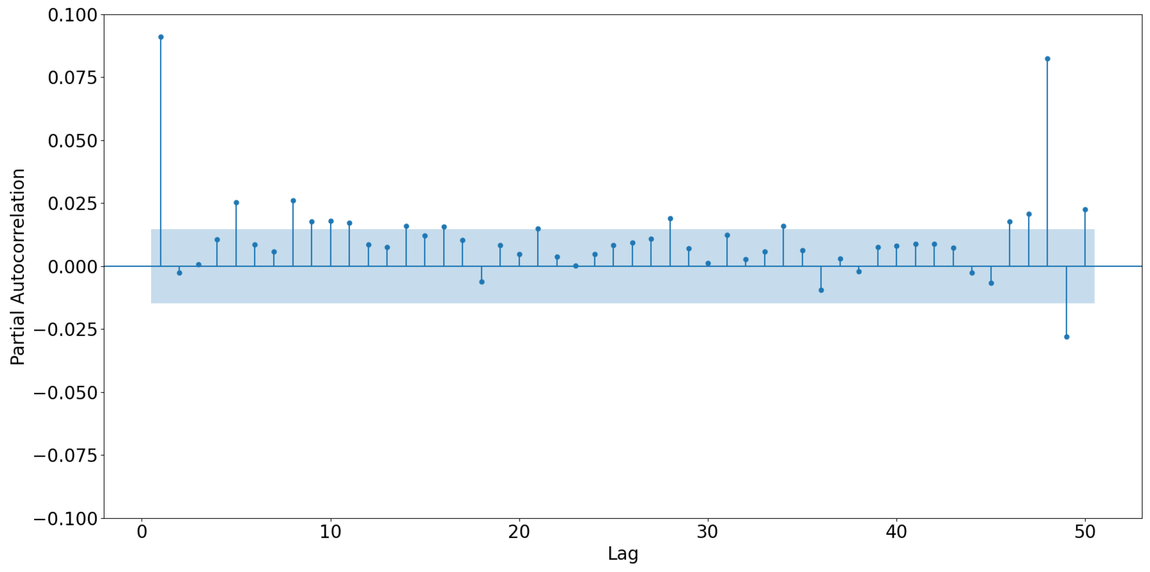
A forecast is optimal when there is no information left in the deviation between the forecasted and the actual variables, and the residuals represents a white noise process ${ϵ}_t$ with $E\left({ϵ}_t\right)=0$. For this purpose, a rolling forecast $\widehat{y}$ with a forecast horizon $h=1$ is created, and the differences from the observed values y are calculated $e=y-\widehat{y}$. This residuals should not exhibit any autocorrelations. To test the optimality of a forecast, Bartlett’s test for white noise with the test statistic $C=ma{x}_{0<r<N/2}\left|S_r-{\displaystyle \frac{r}{N/2}}\right|$ is used. Here, $S_r$ represents the cumulative periodogram, N is the length of the time series, and $r=1,2,\cdots ,N$. $S_r$ is calculated from the Fourier transformations and should scatter around the diagonal to satisfy a uniform distribution when plotted against the frequencies [47]. This analysis is illustrated by applying model M6 to forecast an exemplary RECTS for the entire year 2019, showing the partial autocorrelation (see Figure 13) and Bartlett’s test for white noise (see Figure 14). It is observed that partial autocorrelations at lag 1 and 48 are significantly outside the confidence interval, suggesting a potential relationship at these lags. Since these correlations are weak, with values smaller than 0.1, there is less information remaining in the residuals. On the contrary, Bartlett’s test indicates a non-uniform distribution of frequencies, which may arise from various reasons:

• Seasonal dependency of the residuals magnitude compared to the seasonality in the time series (see Appendix A, Figure A1).
• Insufficiently diverse data observed during forecast model training.
• RECs vary in size regarding their members and have a dynamic portfolio over time, which may cause some issues during forecast model training.
• Since there are a lot of degrees of freedom, e.g., seasonality (annual, weekly, daily) and different REC member compositions, the forecast model is only able to approximately extract domain-invariant features.

Following this analysis for multiple exemplary RECs, Figure A4 in Appendix E indicates a good generalization for various time series characteristics. Most RECs show only minor deviations from the diagonal, with fewer frequencies occurring more frequently.

4.2. Experiment II

This experiment uses the best model setting, M6 (Table 5, Section 4.1), trains a single forecast model for each REC using training data from the year 2018 and applies each one to the test data from the year 2019. Since forecast models are usually trained on single client without using auxiliary information like ${\overrightarrow{r}}_t$, this procedure can be seen as a very good baseline for comparison. In particular, this analysis can determine the impact that including ${\overrightarrow{r}}_t$ and various RECs in the model input data has on forecast accuracy, specifically in terms of non-stationary and discontinuous time series. The results in

Table 8. Means $\mu$ and standard deviations $\sigma$ of the errors from forecast models trained on individual RECs neglecting ${\overrightarrow{r}}_t$ (orange—Single Model) and best forecast model M6 trained on multiple RECs in a federated manner (Table 5, blue—FL Model).

	MAE-$\mathit{\mu }$	MAE-$\mathit{\sigma }$
FL Model	2.65	0.5
Single Model	4.72	0.5

show that forecast model performance greatly benefits from using ${\overrightarrow{r}}_t$ and a big amount of data during model training (federated learned forecast model—FL Model), while neglecting this leads to a significantly larger forecast error (single time series forecast model—Single Model). Moreover, Figure 15 illustrates the distribution of MAE over multiple RECs with large member sizes for both, FL Model and Single Model. Regarding that training and test data are highly NON-IID, only the FL Model is particularly capable of handling this circumstance. The reason for this is that the Single Model severely overfits to seasonality by considering doy in the model input data without taking the effect of ${\overrightarrow{r}}_t$ into account. This evaluation demonstrates the importance of model input data and the quantity of training data, and illustrates the capability of our framework to aggregate knowledge from different clients to improve forecast accuracy of RECTS.

4.3. Experiment III

After Section 4.2 demonstrates bad forecast performances using Single Model, this experiment includes ${\overrightarrow{r}}_t$ as auxiliary information in the model input data to determin if it can benefit from it. Compared to Table 8,

Table 9. Means $\mu$ and standard deviations $\sigma$ of the errors from forecast models trained on individual RECs taking ${\overrightarrow{r}}_t$ into account (Single Model) and best forecast model M6 trained on multiple RECs in a federated manner (Table 5, FL Model).

	MAE-$\mathit{\mu }$	MAE-$\mathit{\sigma }$
FL Model	2.65	0.5
Single Model	5.81	1.22

does not confirm this assumption, as the forecast error, in terms of MAE, increases from $4.72\mathrm{kW}$ to $5.81\mathrm{kW}$. Figure 16 visually demonstrates this measurement, indicating a higher magnitude and higher variability of forecast errors. While the Single Model without ${\overrightarrow{r}}_t$ strongly overfit to the seasonality within the training dataset, the one considering ${\overrightarrow{r}}_t$ attemps to handle both, seasonality with regards to ${\overrightarrow{r}}_t$. Since this further increases the complexity of data processing within the forecast model without providing a variety of samples for specific seasonalities and ${\overrightarrow{r}}_t$, forecast accuracy even worsens. A reason for this is the dynamic evolution of ${\overrightarrow{r}}_t$ (Section 2.2), whose impact on electricity consumption has not been adequately learned in model training due to a lack of data variety. This evaluation further shows that training a forecast model for each individual RECTS, whether using ${\overrightarrow{r}}_t$ or not, is unable to extract domain-invariant features as well as cross-domain behaviors in the context of non-stationary and discontinuous time series. Consequently, both Single Models are not transferable to unseen data. These results confirm that aggregating and extracting relational knowledge from a vast array of diverse data sources is essential to improve forecast accuracy of RECTS.

4.4. Experiment IV

While Section 4.2 and Section 4.3 aim to compare forecast models trained on single data sources with those trained on multiple sources, Experiment IV evaluates forecast accuracies of a centrally learned forecast model (CL Model) against the best FL Model M6 (Section 4.1) using identical data samples. In this case, the CL Model neglects ${\overrightarrow{r}}_t$ to obtain a baseline accuracy measurement for a forecast model, following common ARIX process equations.

Table 10. Means $\mu$ and standard deviations $\sigma$ of the errors from forecast models trained centrally on multiple RECs neglecting ${\overrightarrow{r}}_t$ (CL Model) and best forecast model M6 trained on multiple RECs in a federated manner (Table 5, FL Model).

	MAE-$\mathit{\mu }$	MAE-$\mathit{\sigma }$
FL Model	2.65	0.5
CL Model	3.23	0.48

shows a strong improvement compared to Single Models (Table 8 and Table 9), but it still does not perform as well as the best FL Model M6 (Section 4.1). Although FL Model is trained in a federated manner, it outperforms CL Model by over 18% in terms of MAE. This strongly suggests the usage of auxiliary data to forecast non-stationary and discontinuous RECTS—Figure 17 demonstrates this behavior for every REC. This evaluation once again shows that FL Model can extract domain-invariant features and cross-domain behaviors by utilizing ${\overrightarrow{r}}_t$, resulting in higher forecast accuracies compared to conventional forecast models.

4.5. Experiment V

This section is intended to compare CL Model with FL Model using same training and testing samples, as well as same settings outlined in Section 4.1. While

Table 11. Means $\mu$ and standard deviations $\sigma$ of the errors from forecast models trained centrally on multiple RECs taking ${\overrightarrow{r}}_t$ into account (CL Model) and best forecast model M6 trained on multiple RECs in a federated manner (Table 5, FL Model).

	MAE-$\mathit{\mu }$	MAE-$\mathit{\sigma }$
FL Model	2.65	0.5
CL Model	2.86	0.43

shows slightly better results for FL Model, Figure 18 illustrates no significant differences in error measurements. These results strongly prove the capability of our framework to forecast non-stationary and discontinous RECTS, when training a forecast model by applying FL. Moreover, it is able to extract domain-invariant features and cross-domain behaviors as good as a central learned model.

5. Discussion

This work introduces the European energy market, with a particular emphasis on dynamic portfolios of RECs, which have the potential to introduce new business models, enhance energy efficiency, and reduce electricity costs for their members. Besides fostering energy sharing (tenant electricity, electric vehicle charging, etc.), dynamic portfolios also contain risks concerning energy management tasks, e.g., forecasting energy demand or optimizing the energy system including demand side management, which could lead to financial losses, stress on the grid, operational inefficiencies, and member dissatisfaction. The goal of this work is to develop a forecast framework that overcomes non-stationary, discontinuous, and NON-IID time series.

Since no real data is available, we synthesize RECTS by initially creating numerous district time series with diverse characteristics and subsequently aggregating them time-dependently. Given only this type of data, we can only simulate the forecasting of RECTS approximately. Various analyses confirm that the generated time series are non-stationary, discontinuous, and NON-IID, as these attributes are prerequisites of the research question. Daily portfolio changes may appear extreme, but they can occur if there is a company whose business model involves automatically optimizing portfolios based on the day of the week, accounting for varying patterns of electricity consumption and generation.

To create model input arrays, we refer closely to ARIX time series processing equations, omitting the differencing filter, as neural networks are capable of automatically extracting this feature. Since the composition of residents in RECs might change daily, we divide these arrays into past, present, and future ones. Thereby, we clearly describe the engineering of calendar data to include temporal dependencies of RECTS. To determine the effect of residents composition on RECTS characteristics, we assume that we possess this information for all RECs and days. While such information does not actually exist, we must first label each member time series within a REC by using a sophisticated classification algorithm.

We then develop a forecasting model based on a FNN architecture with three input layers, each taking into account a separate input array representing a specific time interval within the time series process. As each layer extracts latent features across various time horizons, the forecasting model is capable of handling dynamic portfolios. As our primary objective is to analyze the feasibility of a forecasting model trained using FL, we omit considerations of other neural network architectures, such as sequence-to-sequence networks or temporal convolutional networks which might result in better forecast accuracies. Furthermore, we omit hyperparameter optimization regarding the activation function, the number of neurons, and the number of hidden layers to identify optimal settings.

To train a forecasting model across multiple clients with FL, we employ Federated Averaging exclusively for updating model weights, and use stochastic gradient descent for local model training. Additionally, we apply only one training epoch on each client and experiment with various configurations regarding data sharing, batch size, and learning rate to mitigate weight divergence issues. In contrast, we did not consider techniques such as FedProx [48] and FedDyn [49] that involve the regularization of model weight updates, learning rate degradation [49,50], layer-wise training [51], and a varying quantity of training data samples [50]. Since model convergence strongly depends on the interaction between sample size, batch size, and learning rate, this issue was be analyzed and by a more in-depth optimization, there could be significant potential for improvement in model convergence and performance.

Additionally, we perform multiple training sessions of the forecasting model using FL, taking into account various configurations related to the number of shared time series, the learning rate, and the batch size in order to determine the best setting. This one is subsequently applied in similar experiments to demonstrate the effectiveness of our framework, showing that the FL Model and the CL Model have nearly identical performance. Hence, our framework is capable of aggregating knowledge from multiple clients, learning domain-invariant features, and extracting cross-domain behaviors through the application of FL. Moreover, it is transferable to new unseen data. Nevertheless, more sensitivity studies on hyperparameter tuning must be conducted, e.g., testing the required quantity of RECTS to extract the relational knowledge necessary to cause failure, and the application in a real-world scenario should be analyzed. Since the number of RECs could potentially increase significantly, there could be advantages in using FL regarding training time.

In comparison to similar studies, we not only evaluate our framework using generic error metrics like MAE or RMSE, but also focus intensively on remaining frequencies in the residuals (compare with [38,39,41,42]). Since many different RECs could potentially participate in such a forecasting community, some might suffer from data poisoning attacks. In this case, the FL framework should detect and correct anomalies in each time series to ensure robust forecast model training [52,53].

While this research proposes a method to train a forecast model for non-stationary, discontinuous, and NON-IID time series across multiple clients, several challenges remain for deploying FL in large-scale systems. Each client may possess different hardware configurations regarding smart meters, data management systems, CPUs, and GPUs, potentially leading to communication issues. To address these issues and ensure interoperability, it is recommended to aggregate model weights asynchronously. Furthermore, there is a need for standardized protocols and APIs that enable seamless participation of various data management systems in FL. This includes standardizing data access, processing, and updating methods within the FL context, using techniques such as homomorphic encryption or differential privacy [54]. As participating clients may have time series data with varying temporal resolutions, quality, and quantities, data pre-processing steps such as missing value substitution or anomaly detection must be adapted accordingly. Intelligent weight averaging algorithms like FedProx [48] and FedDyn [49] can help to reduce communication overhead, improving the overall efficiency and robustness of the FL system.

Since our approach can extract domain-invariant features and identify correlations between domains based on temporal and exogenous variables, it can also be applied to time series data from other sectors such as retail, e-commerce, and financial markets. Economic data generally exhibit cycles and trends due to factors like financial crises, policy changes, and technological innovations. Utilizing extensive labeled or structural data that approximately describes the entire ecosystem could enable more accurate predictions of future changes, thereby minimizing financial risks.

6. Conclusions

This work examines various forecasting strategies to handle non-stationary, discontinous, and NON-IID time series across distributed clients. After generating a sufficient number of electricity consumption time series for Renewable Energy Communities with dynamic customer portfolios, several data pre-processing methods are tested in conjunction with differently configured forecast model training on either single or multiple time series. Our novel forecasting framework demonstrates the effectiveness of data sharing to learn domain-invariant features and cross-domain behaviors by aggregating knowledge from various data sources using federated learning. Besides ensuring transferability to unseen data, the forecast accuracy is nearly identical to that of a centrally trained forecasting model. Our novel framework possesses the potential to revolutionize electricity demand forecasting for decentralized energy systems by identifying effective training settings. Since there is still some remaining information in the residuals, future work will focus on intelligent data pre-processing and complex forecasting model architectures to fully extract domain-invariant features. Moreover, this framework needs to be deployed in real-world applications to validate its performance on non-synthetic data. Lastly, appropriate classification algorithms have to be developed to generate time series labels, which can be used as auxiliary information in the model’s input space.

References

1. Available online: https://www.ipcc.ch/sr15/chapter/chapter-1/ (accessed on 7 February 2024).
2. Available online: https://www.europarl.europa.eu/factsheets/de/sheet/45/energiebinnenmarkt (accessed on 5 January 2023).
3. Available online: https://eur-lex.europa.eu/legal-content/DE/TXT/PDF/?uri=CELEX:02018L2001-20181221&from=EN (accessed on 5 January 2023).
4. Available online: https://www.bmwk.de/Redaktion/DE/Publikationen/Energie/7-energieforschungsprogramm-der-bundesregierung.pdf?__blob=publicationFile&v=4 (accessed on 5 January 2023).
5. Sauerbrey, J.; Bender, T.; Flemming, S.; Martin, A.; Naumann, S.; Warweg, O. Towards intelligent energy management in energy communities: Introducing the district energy manager and an IT reference architecture for district energy management systems. Energy Rep. 2024, 11, 2255–2265. [Google Scholar] [CrossRef]
6. Abrahamse, W.; Steg, L. Factors Related to Household Energy Use and Intention to Reduce It: The Role of Psychological and Socio-Demographic Variables. Hum. Ecol. Rev. 2011, 18, 30–40. [Google Scholar]
7. Flemming, S.; Bender, T.; Surmann, A.; Pelka, S.; Martin, A.; Kuehnbach, M. Vor-Ort-Systeme Als Flexibler Baustein im Energiesystem? Eine cross-sektorale Potenzialanalyse; Fraunhofer IOSB-AST: Ilmenau, Germany, 2023. [Google Scholar] [CrossRef]
8. Beucker, S.; Bergesen, J.; Gibon, T. Building Energy Management Systems: Global Potentials and Environmental Implications of Deployment. J. Ind. Ecol. 2015, 20, 223–233. [Google Scholar] [CrossRef]
9. Available online: https://wirtschaftslexikon.gabler.de/definition/energiemanagementsystem-53996 (accessed on 6 January 2023).
10. Richter, L.; Lehna, M.; Marchand, S.; Scholz, C.; Dreher, A.; Klaiber, S.; Lenk, S. Artificial Intelligence for Electricity Supply Chain automation. Renew. Sustain. Energy Rev. 2022, 163, 112459. [Google Scholar] [CrossRef]
11. Available online: https://www.gesetze-im-internet.de/enwg_2005/__41a.html (accessed on 7 February 2024).
12. Klaiber, S. Analyse, Identifikation und Prognose Preisbeeinflusster Elektrischer Lastzeitreihen. Ph.D. Thesis, Technische Universität Ilmenau, Ilmenau, Germany, 2020. [Google Scholar]
13. Available online: https://eur-lex.europa.eu/legal-content/en/TXT/?uri=CELEX:32019L0944 (accessed on 7 February 2024).
14. Hyndman, R.; Athanasopoulos, G. Forecasting: Principles and Practice, 2nd ed.; OTexts: Melbourne, Australia, 2018. [Google Scholar]
15. Richter, L.; Bender, T.; Lenk, S.; Bretschneider, P. Generating Synthetic Electricity Load Time Series at District Scale Using Probabilistic Forecasts. Energies 2024, 17, 1634. [Google Scholar] [CrossRef]
16. Han, Z.; Zhao, J.; Leung, H.; Ma, K.F.; Wang, W. A Review of Deep Learning Models for Time Series Prediction. IEEE Sens. J. 2021, 21, 7833–7848. [Google Scholar] [CrossRef]
17. Runge, J.; Zmeureanu, R. A Review of Deep Learning Techniques for Forecasting Energy Use in Buildings. Energies 2021, 14, 608. [Google Scholar] [CrossRef]
18. Bot, K.; Ruano, A.; Ruano, M. Forecasting Electricity Consumption in Residential Buildings for Home Energy Management Systems; Springer International Publishing: Cham, Switzerland, 2020; pp. 313–326. [Google Scholar] [CrossRef]
19. Wang, W.; Hussain, F.; Lian, Z.; Yin, Z.; Gadekallu, T.; Pham, Q.V.; Dev, K.; Su, C. Secure-Enhanced Federated Learning for AI-Empowered Electric Vehicle Energy Prediction. IEEE Consum. Electron. Mag. 2021, 12, 27–34. [Google Scholar] [CrossRef]
20. Lu, Y.; Tian, Z.; Zhou, R.; Liu, W. A general transfer learning-based framework for thermal load prediction in regional energy system. Energy 2021, 217, 119322. [Google Scholar] [CrossRef]
21. Suryanarayana, G.; Lago, J.; Geysen, D.; Aleksiejuk, P.; Johansson, C. Thermal load forecasting in district heating networks using deep learning and advanced feature selection methods. Energy 2018, 157, 141–149. [Google Scholar] [CrossRef]
22. Shirzadi, N.; Nizami, A.; Khazen, M.; Nik Bakht, M. Medium-Term Regional Electricity Load Forecasting through Machine Learning and Deep Learning. Designs 2021, 5, 27. [Google Scholar] [CrossRef]
23. Liu, H.; Zhang, X.; Shen, X.; Sun, H. A Federated Learning Framework for Smart Grids: Securing Power Traces in Collaborative Learning. arXiv 2021, arXiv:2103.11870. [Google Scholar]
24. Taïk, A.; Cherkaoui, S. Electrical Load Forecasting Using Edge Computing and Federated Learning. In Proceedings of the ICC 2020—2020 IEEE International Conference on Communications (ICC), Dublin, Ireland, 7–11 June 2020; pp. 1–6. [Google Scholar] [CrossRef]
25. Gholizadeh, N.; Musilek, P. Federated learning with hyperparameter-based clustering for electrical load forecasting. Internet Things 2021, 17, 100470. [Google Scholar] [CrossRef]
26. Available online: https://www.caci.co.uk/wp-content/uploads/2021/06/Acorn-User-Guide-2020.pdf (accessed on 16 May 2024).
27. Gardner, W.A.; Napolitano, A.; Paura, L. Cyclostationarity: Half a century of research. Signal Process. 2006, 86, 639–697. [Google Scholar] [CrossRef]
28. Aminikhanghahi, S.; Cook, D. A Survey of Methods for Time Series Change Point Detection. Knowl. Inf. Syst. 2017, 51, 339–367. [Google Scholar] [CrossRef] [PubMed]
29. Schwertman, N.C.; Owens, M.A.; Adnan, R. A simple more general boxplot method for identifying outliers. Comput. Stat. Data Anal. 2004, 47, 165–174. [Google Scholar] [CrossRef]
30. Pinheiro, M.; Madeira, S.; Francisco, A. Short-term electricity load forecasting—A systematic approach from system level to secondary substations. Appl. Energy 2023, 332, 120493. [Google Scholar] [CrossRef]
31. Gasparin, A.; Lukovic, S.; Alippi, C. Deep Learning for Time Series Forecasting: The Electric Load Case. arXiv 2019, arXiv:1907.09207. [Google Scholar] [CrossRef]
32. Tunnicliffe Wilson, G. Time Series Analysis: Forecasting and Control, 5th Edition, by George E. P. Box, Gwilym M. Jenkins, Gregory C. Reinsel and Greta M. Ljung, 2015. Published by John Wiley and Sons Inc., Hoboken, New Jersey, pp. 712. ISBN: 978-1-118-67502-1. J. Time Ser. Anal. 2016, 37, 709–711. [Google Scholar] [CrossRef]
33. Shi, Y.; Ying, X.; Yang, J. Deep Unsupervised Domain Adaptation with Time Series Sensor Data: A Survey. Sensors 2022, 22, 5507. [Google Scholar] [CrossRef]
34. Purushotham, S.; Carvalho, W.; Nilanon, T.; Liu, Y. Variational Recurrent Adversarial Deep Domain Adaptation. In Proceedings of the International Conference on Learning Representations, New Orleans, LA, USA, 6–9 May 2019. [Google Scholar]
35. Arik, S.O.; Yoder, N.C.; Pfister, T. Self-Adaptive Forecasting for Improved Deep Learning on Non-Stationary Time-Series. arXiv 2022, arXiv:2202.02403. [Google Scholar]
36. Available online: https://transparency.entsoe.eu (accessed on 28 November 2023).
37. McMahan, H.B.; Moore, E.; Ramage, D.; Hampson, S.; y Arcas, B.A. Communication-Efficient Learning of Deep Networks from Decentralized Data. arXiv 2023, arXiv:1602.05629. [Google Scholar]
38. Shi, Y.; Xu, X. Deep Federated Adaptation: An Adaptative Residential Load Forecasting Approach with Federated Learning. Sensors 2022, 22, 3264. [Google Scholar] [CrossRef]
39. Wang, Y.; Gao, N.; Hug, G. Personalized Federated Learning for Individual Consumer Load Forecasting. CSEE J. Power Energy Syst. 2023, 9, 326–330. [Google Scholar] [CrossRef]
40. Chen, J.; Gao, T.; Si, R.; Dai, Y.; Jiang, Y.; Zhang, J. Residential Short Term Load Forecasting Based on Federated Learning. In Proceedings of the 2022 IEEE 2nd International Conference on Digital Twins and Parallel Intelligence (DTPI), Boston, MA, USA, 24–28 October 2022; pp. 1–6. [Google Scholar] [CrossRef]
41. Savi, M.; Olivadese, F. Short-Term Energy Consumption Forecasting at the Edge: A Federated Learning Approach. IEEE Access 2021, 9, 1–21. [Google Scholar] [CrossRef]
42. Yang, Y.; Wang, Z.; Zhao, S.; Wu, J. An integrated federated learning algorithm for short-term load forecasting. Electr. Power Syst. Res. 2023, 214, 108830. [Google Scholar] [CrossRef]
43. Zhu, H.; Xu, J.; Liu, S.; Jin, Y. Federated Learning on Non-IID Data: A Survey. arXiv 2021, arXiv:2106.06843. [Google Scholar] [CrossRef]
44. Zhao, Y.; Li, M.; Lai, L.; Suda, N.; Civin, D.; Chandra, V. Federated Learning with Non-IID Data. arXiv 2018, arXiv:1806.00582. [Google Scholar] [CrossRef]
45. Keskar, N.S.; Mudigere, D.; Nocedal, J.; Smelyanskiy, M.; Tang, P.T.P. On Large-Batch Training for Deep Learning: Generalization Gap and Sharp Minima. arXiv 2017, arXiv:1609.04836. [Google Scholar]
46. Available online: https://www.tensorflow.org (accessed on 13 March 2024).
47. Schlittgen, R.; Streitberg, B.H. Zeitreihenanalyse; Oldenbourg Wissenschaftsverlag: Munich, Germany, 2001. [Google Scholar] [CrossRef]
48. Li, T.; Sahu, A.K.; Zaheer, M.; Sanjabi, M.; Talwalkar, A.; Smith, V. Federated Optimization in Heterogeneous Networks. arXiv 2020, arXiv:1812.06127. [Google Scholar]
49. Acar, D.A.E.; Zhao, Y.; Navarro, R.M.; Mattina, M.; Whatmough, P.N.; Saligrama, V. Federated Learning Based on Dynamic Regularization. arXiv 2021, arXiv:2111.04263. [Google Scholar]
50. Li, X.; Huang, K.; Yang, W.; Wang, S.; Zhang, Z. On the Convergence of FedAvg on Non-IID Data. arXiv 2020, arXiv:1907.02189. [Google Scholar]
51. Charles, Z.; Garrett, Z.; Huo, Z.; Shmulyian, S.; Smith, V. On Large-Cohort Training for Federated Learning. arXiv 2021, arXiv:2106.07820. [Google Scholar]
52. VandenHeuvel, D.; Wu, J.; Wang, Y.G. Robust regression for electricity demand forecasting against cyberattacks. Int. J. Forecast. 2023, 39, 1573–1592. [Google Scholar] [CrossRef]
53. Manzoor, H.U.; Khan, A.R.; Flynn, D.; Alam, M.M.; Akram, M.; Imran, M.A.; Zoha, A. FedBranched: Leveraging Federated Learning for Anomaly-Aware Load Forecasting in Energy Networks. Sensors 2023, 23, 3570. [Google Scholar] [CrossRef]
54. Xu, C.; Qu, Y.; Xiang, Y.; Gao, L. Asynchronous Federated Learning on Heterogeneous Devices: A Survey. arXiv 2023, arXiv:2109.04269. [Google Scholar] [CrossRef]
Figure 1. Time-variant portfolios C 0 , C 1 , C 2 , C 3 , C 4 , C 5 of RECs.
Smartcities 07 00082 g001
Figure 2. Illustrating two dimensional principal components of X c o v , clustered with K-means and number of clusters k = 10 . Each color represents subgroups belonging to one cluster, while thick points depict the central subgroups within each cluster.
Smartcities 07 00082 g002
Figure 3. Resulting time series (with x-axis dates in the format YYYY-MM) after removing seasonality, periodicity and trend at 12:00.
Smartcities 07 00082 g003
Figure 4. Boxplot showing distributions of differential time series for every week of year in the dataset.
Smartcities 07 00082 g004
Figure 5. Heatmap of correlation matrix X r e c , c o r r using RECTS as input, showing different electrical consumption behaviors of all RECs.
Smartcities 07 00082 g005
Figure 7. Principle neural network architecture, utilizing Tensorflow Keras Dense layers (orange) three times within the input space L 1 A R , L 1 I , L 1 F to handle past X I , present X A R and future X F data (blue) separately and one in the output space L 2 to fit future values of the target variable (blue) Y F .
Smartcities 07 00082 g007
Figure 8. The evolution of model weights across local training epochs t 0 , t 1 , t 2 , t 3 , under both independent and identically distributed (iid) and NON-IID data scenarios, demonstrates diverging weight patterns (inspired by [44]).
Smartcities 07 00082 g008
Figure 10. Illustration of the process of conducting various experiments: (1) Conduct various FL runs within experiment I. using different configurations concerning shared time series, batch size, and learning rate, (2) extract best configuration from experiment I. and apply it within experiments II–V, (3) compare and evaluate results.
Smartcities 07 00082 g010
Figure 11. MAE for models M0, M1, M2, M3, M4, M5, M6, M7 applied on test data, depending on the number of federated learning epochs.
Smartcities 07 00082 g011
Figure 12. Time series forecasts for an exemplary RECTS visualized as a scatter plot (a) and a line plot (b) with x-axis dates in the format YYYY-MM-DD, using the best forecast model M6.
Smartcities 07 00082 g012
Figure 13. Partial autocorrelation of the residuals using Python statsmodels package. The 95% confidence interval is shown as a shaded region, with dots outside indicating significant correlations.
Smartcities 07 00082 g013
Figure 14. Bartlett’s test for white noise on exemplary RECTS.
Smartcities 07 00082 g014
Figure 15. MAE of forecast models referred to individual RECs neglecting r t (orange—Single Model) compared to the best FL model M6 (blue—FL Model) from Section 4.1.
Smartcities 07 00082 g015
Figure 16. MAE of forecast models referred to individual RECs taking r t into account (orange—Single Model) compared to the best FL model M6 (blue—FL Model) from Section 4.1.
Smartcities 07 00082 g016
Figure 17. MAE of a centralized learned forecast model neglecting r t (orange—CL Model) compared to the best FL model M6 (blue—FL Model) from Section 4.1.
Smartcities 07 00082 g017
Figure 18. MAE of a centralized learned forecast model taking r t into account (orange—CL Model) compared to the best FL model M6 (blue—FL Model) from Section 4.1.
Smartcities 07 00082 g018