


An Urban Acoustic Rainfall Estimation Technique Using a CNN Inversion Approach for Potential Smart City Applications


 , , and
Abstract
:1. Introduction
2. Methodology
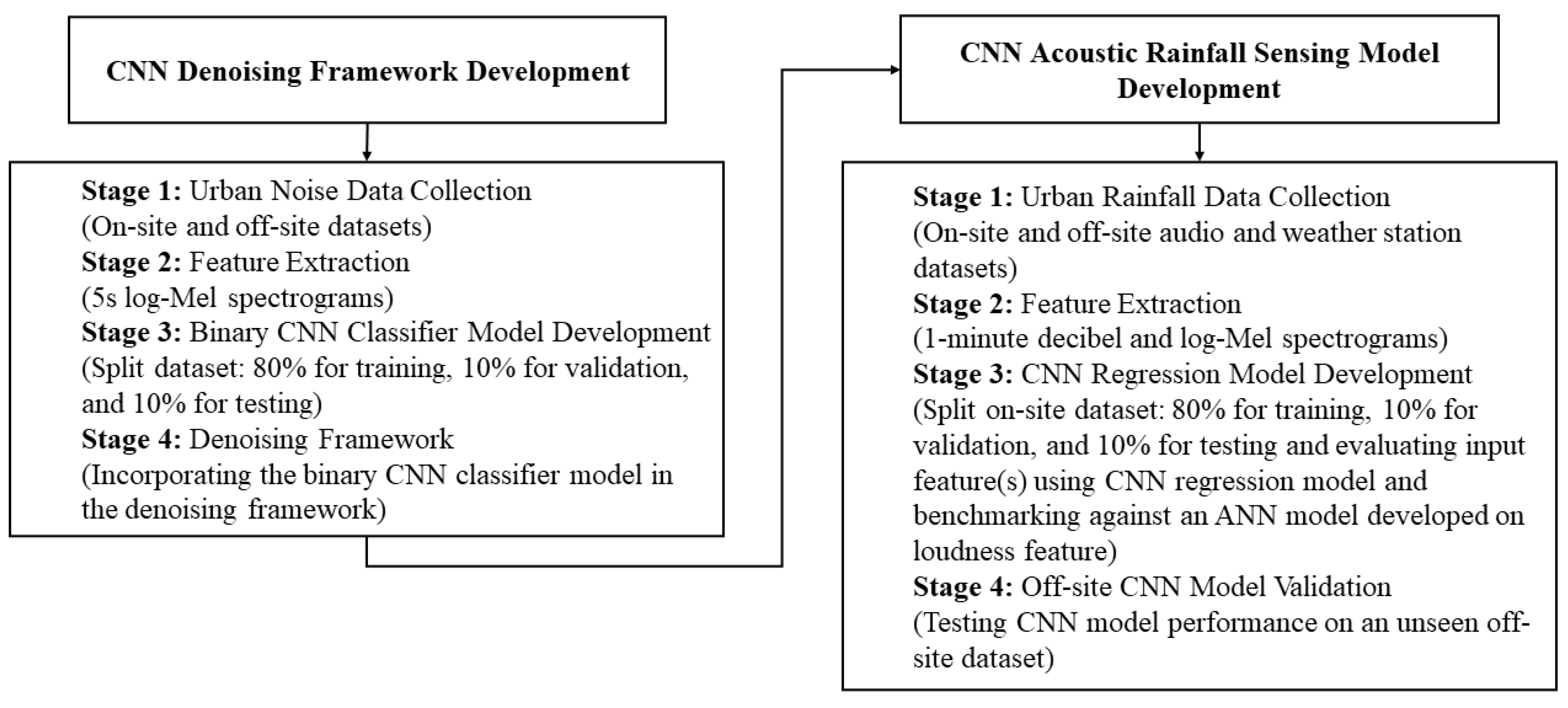
2.1. Overview
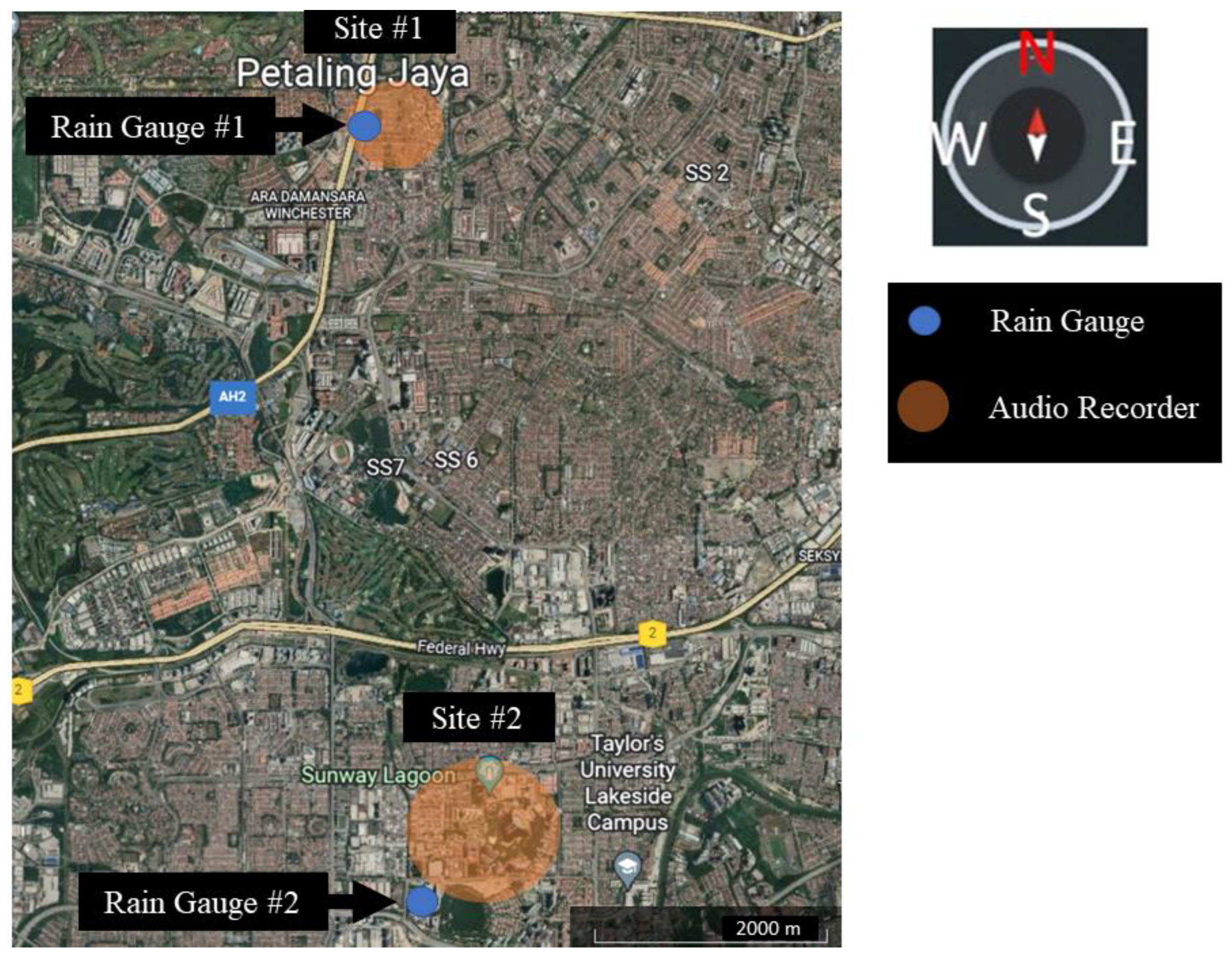
2.2. Study Site and Data Collection
2.2.1. On-Site Calibration and Validation Dataset

2.2.2. Off-Site Validation Dataset
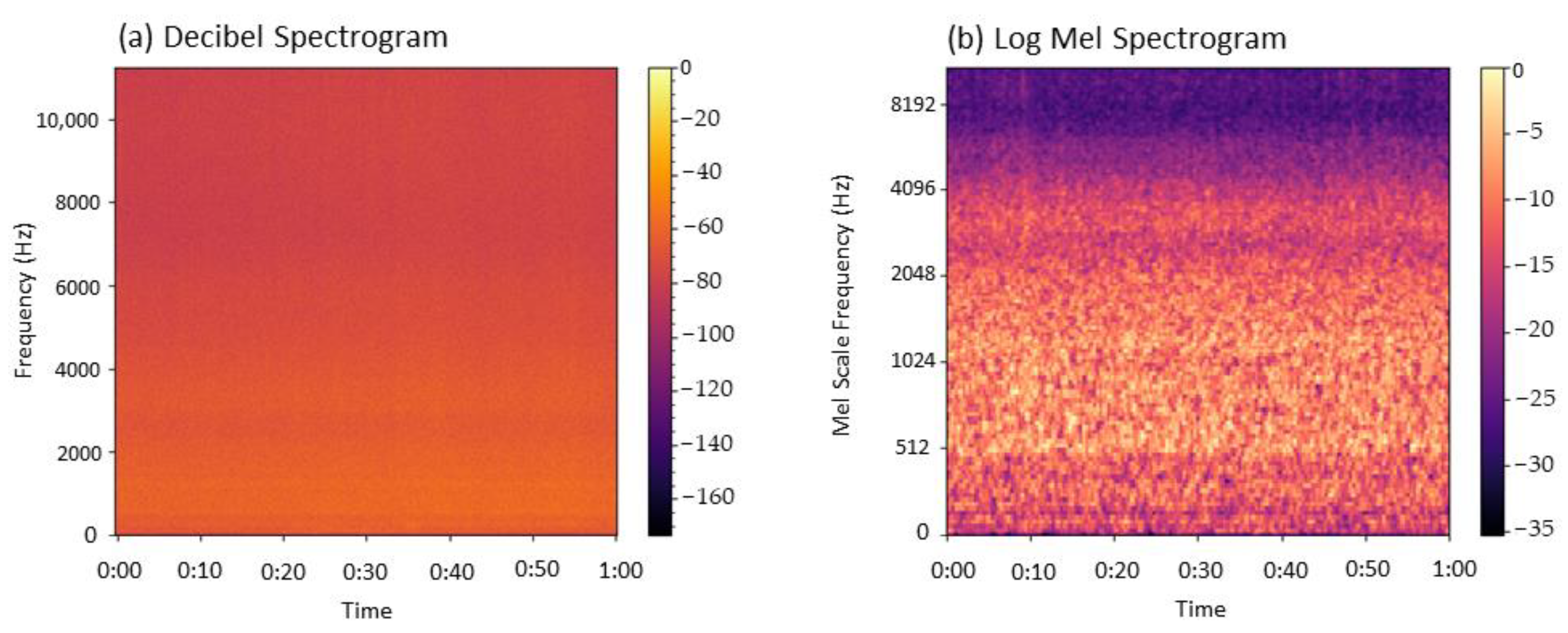
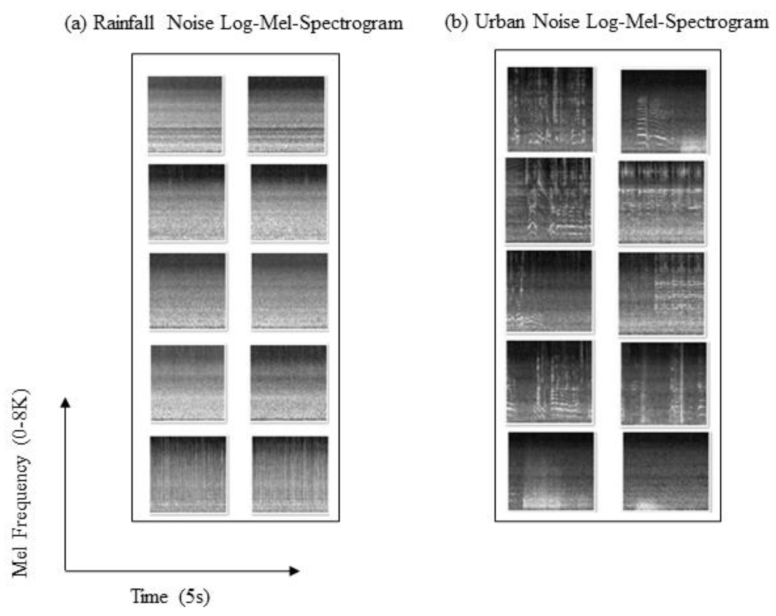
2.3. Acoustic Feature Representation
2.4. Convolutional Neural Networks
2.5. CNN-Based Urban Rainfall Denoising Framework Development
2.6. Acoustic Rainfall Sensing Model Development
2.6.1. Baseline Model
2.6.2. CNN-Based Acoustic Rainfall Sensing Model
2.7. Loss Functions
2.8. Performance Criteria
2.8.1. CNN-Based Urban Rainfall Denoising Model
- Accuracy percentage (%) calculated using Equation (11):
- Recall percentage calculated using Equation (12):
- Specificity percentage calculated using Equation (13):
- Precision percentage calculated using Equation (14):where TN is the true negative value, TP is the true positive value, FN is the false negative value, and FP is the false positive value.
2.8.2. CNN-Based Acoustic Rainfall Sensing Model
- Coefficient of determination (R2) calculated using Equation (15):
- Root mean square error (RMSE) calculated using Equation (16):
- Mean absolute error (MAE) calculated using Equation (17):where and are the observed and simulated rainfall values, respectively; and are the average observed and simulated rainfall values, respectively; and n is the total number of observations.
3. Results and Discussions
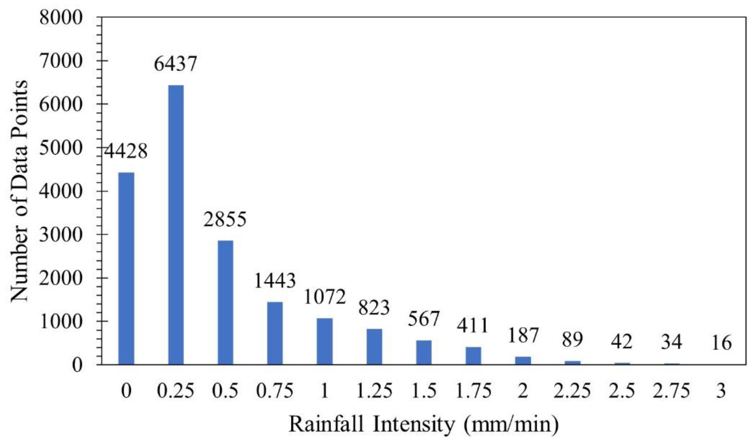
3.1. Rainfall Data Analysis
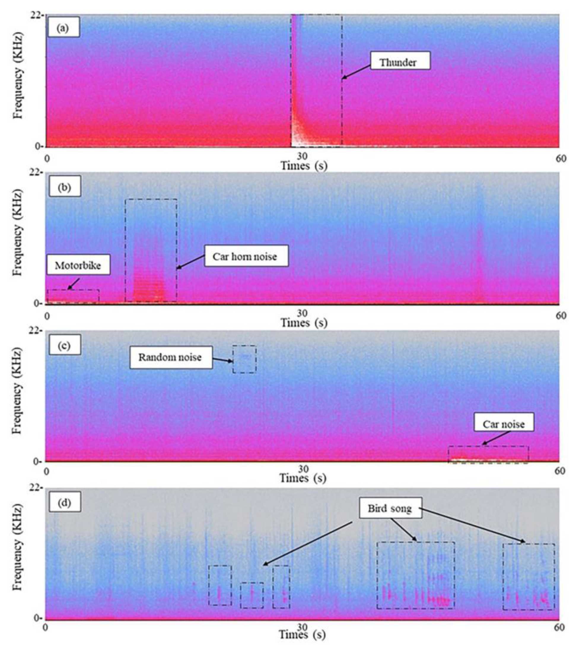
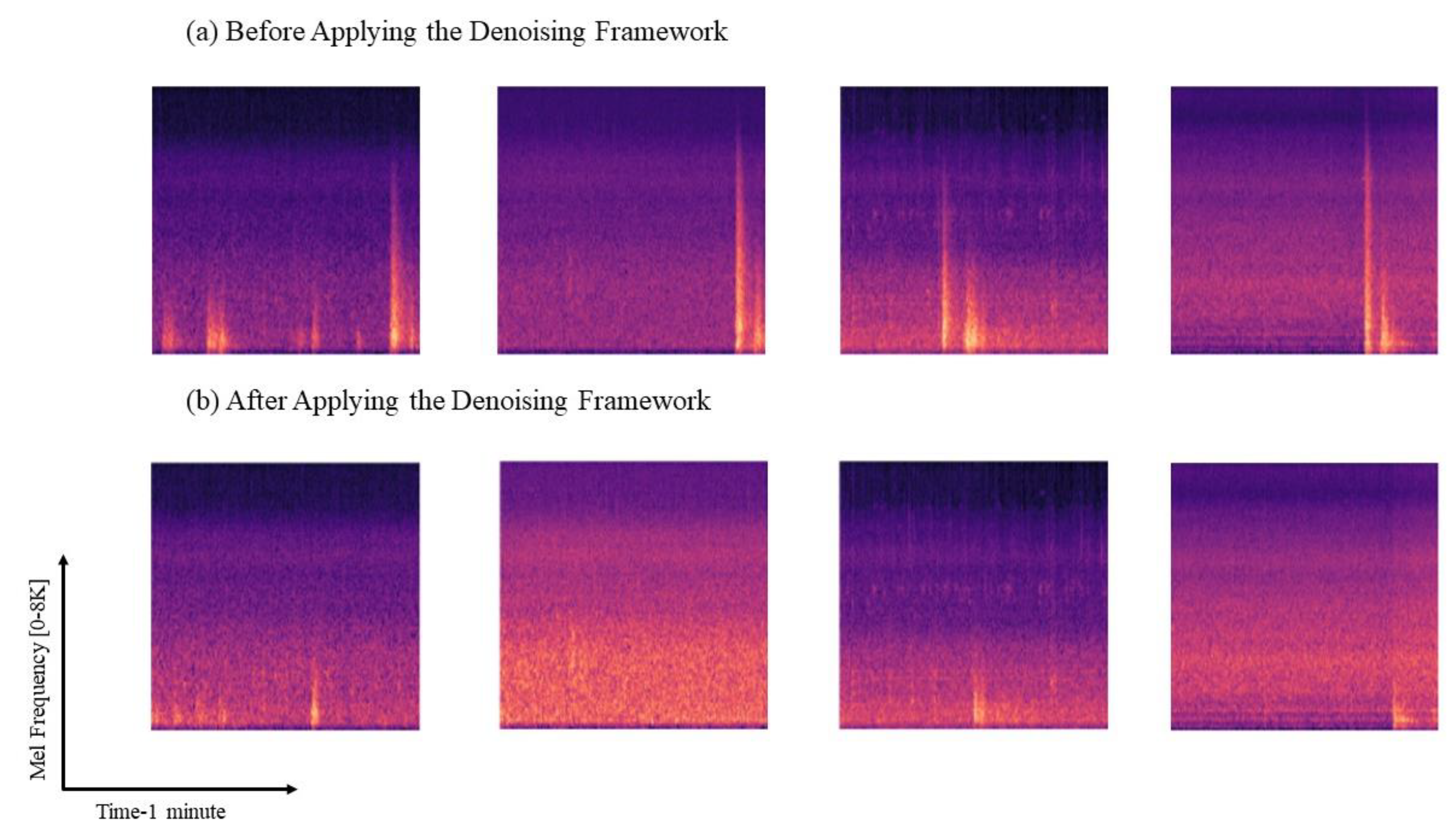
3.2. CNN-Based Urban Acoustic Denoising Framework
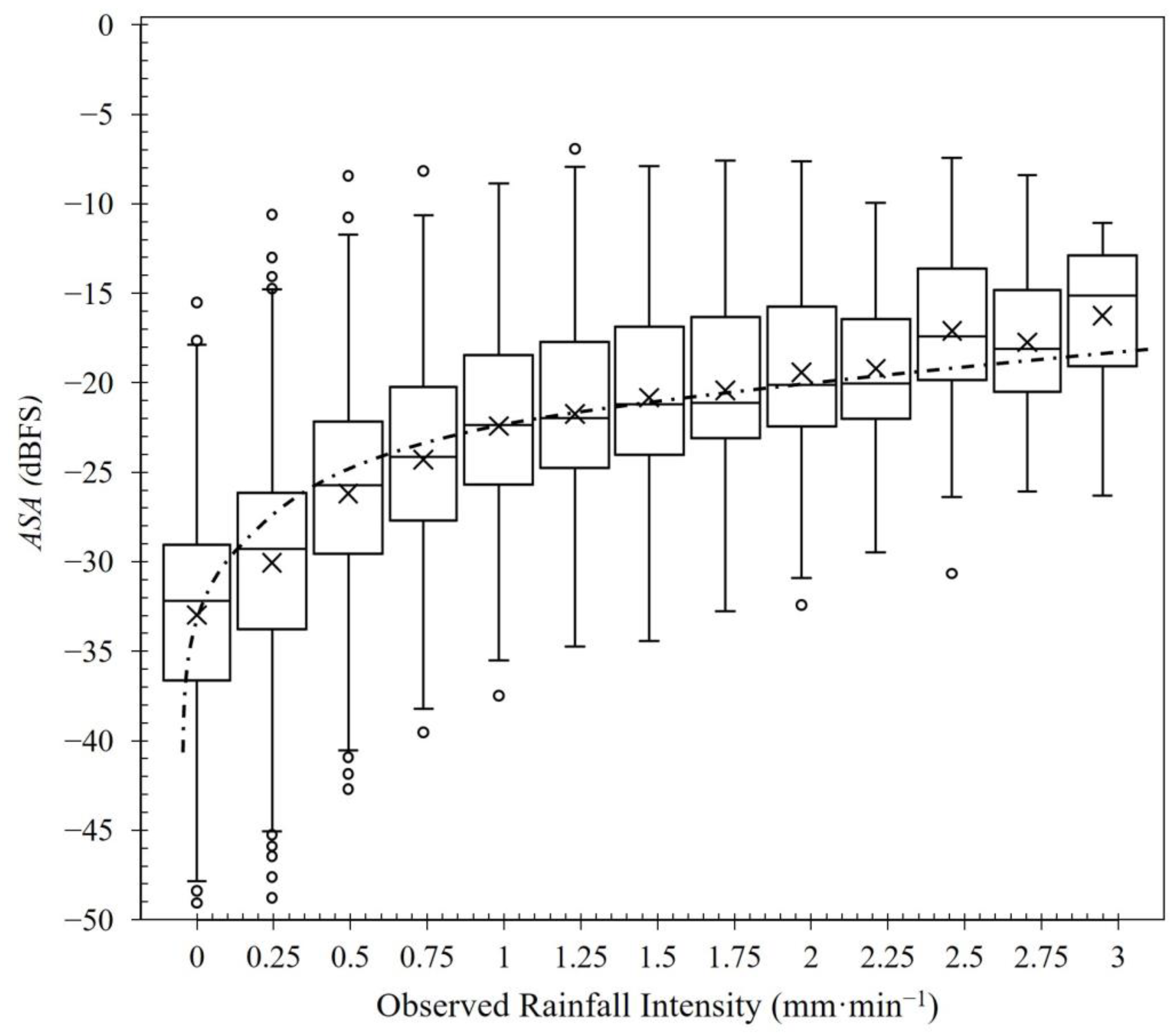
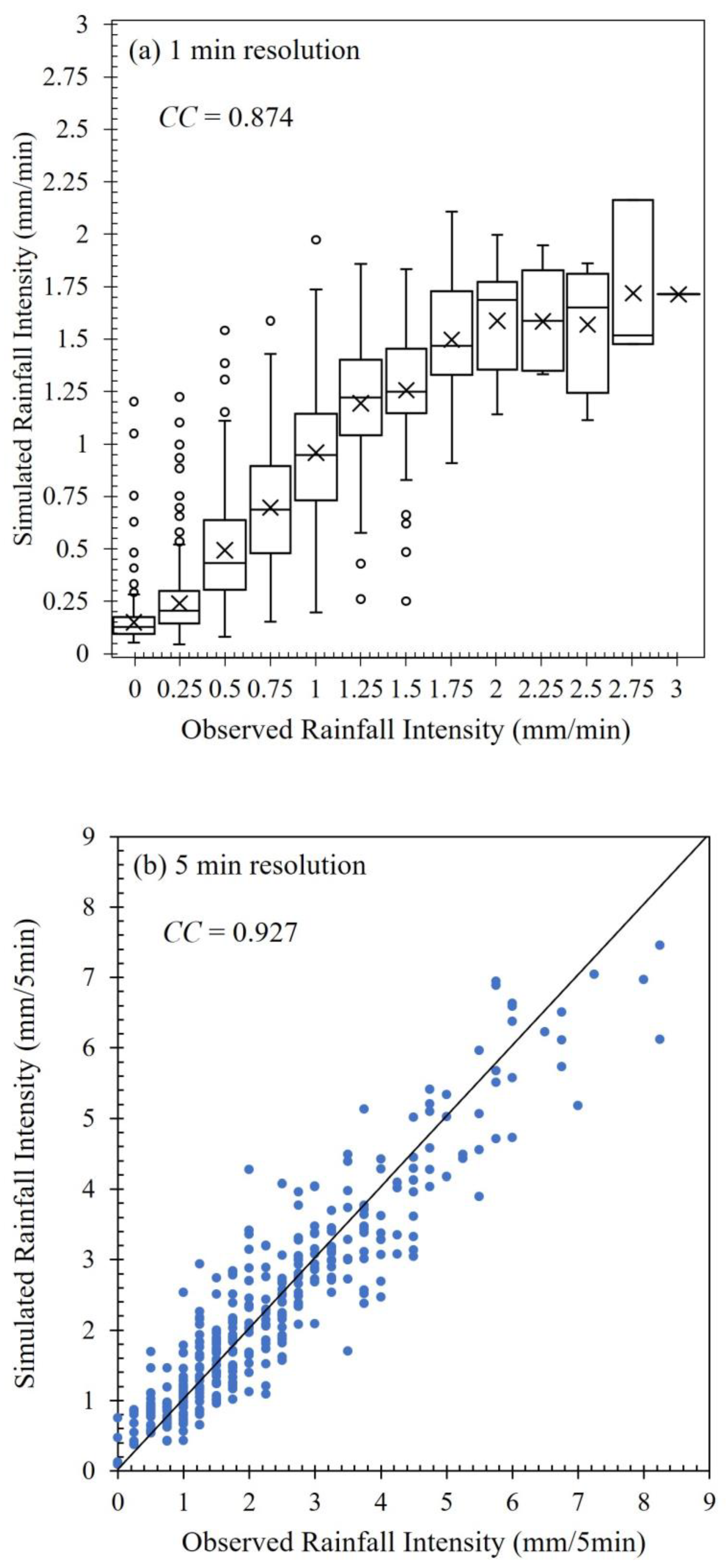
3.3. CNN-Based Acoustic Rainfall Sensing Model
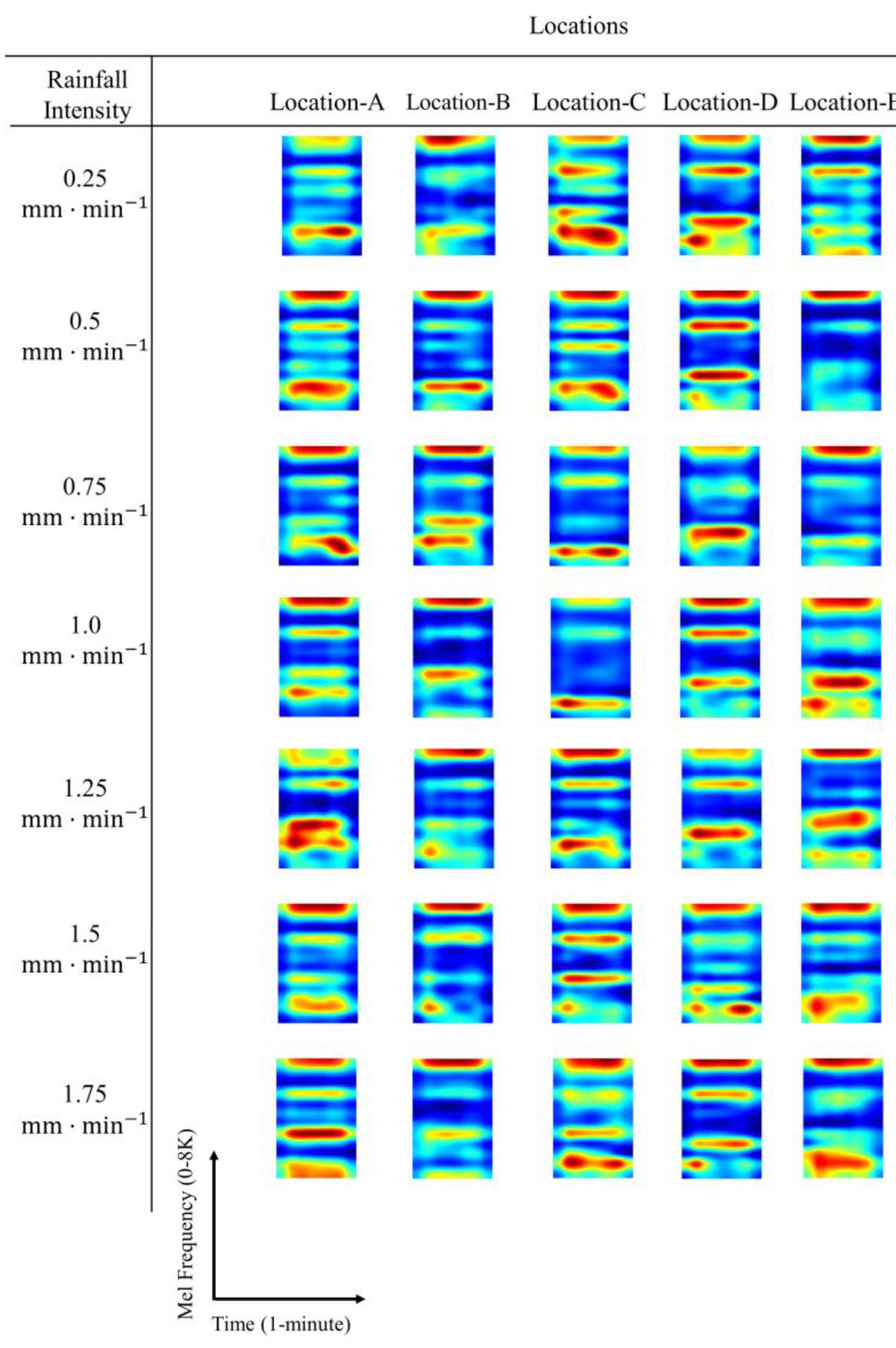
3.4. Local CNN Explainability
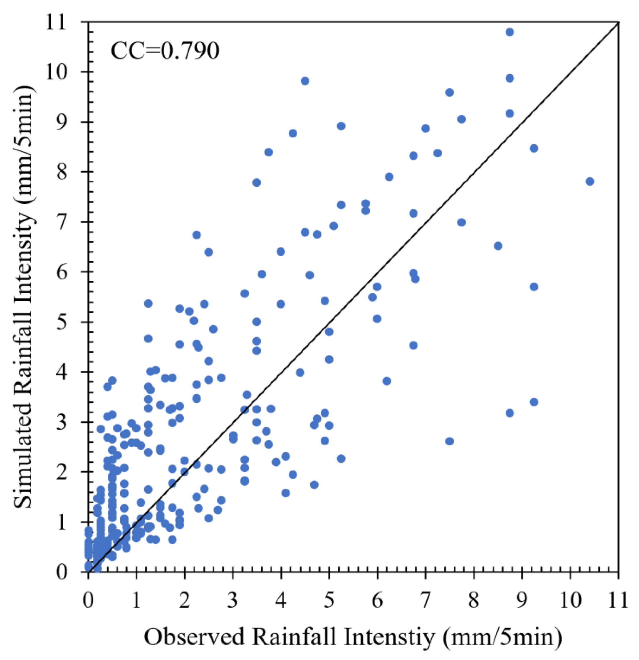
3.5. Potential Application in Citizen Science—Proof of Concept
4. Conclusions and Future Works
Supplementary Materials
Author Contributions
Funding
Data Availability Statement
Acknowledgments
Conflicts of Interest
References
- Gracias, J.S.; Parnell, G.S.; Specking, E.; Pohl, E.A.; Buchanan, R. Smart Cities—A Structured Literature Review. Smart Cities 2023, 6, 1719–1743. [Google Scholar] [CrossRef]
- Wu, W.; Lin, Y. The impact of rapid urbanization on residential energy consumption in China. PLoS ONE 2022, 17, e0270226. [Google Scholar] [CrossRef] [PubMed]
- Chen, H.; Jia, B.; Lau, S.Y. Sustainable urban form for Chinese compact cities: Challenges of a rapid urbanized economy. Habitat. Int. 2008, 32, 28–40. [Google Scholar] [CrossRef]
- Deng, J.S.; Wang, K.; Hong, Y.; Qi, J.G. Spatio-temporal dynamics and evolution of land use change and landscape pattern in response to rapid urbanization. Landsc. Urban Plan. 2009, 92, 187–198. [Google Scholar] [CrossRef]
- Damadam, S.; Zourbakhsh, M.; Javidan, R.; Faroughi, A. An Intelligent IoT Based Traffic Light Management System: Deep Reinforcement Learning. Smart Cities 2022, 5, 1293–1311. [Google Scholar] [CrossRef]
- Calvillo, C.F.; Sánchez-Miralles, A.; Villar, J. Energy management and planning in smart cities. Renew. Sustain. Energy Rev. 2016, 55, 273–287. [Google Scholar] [CrossRef]
- Mingaleva, Z.; Vukovic, N.; Volkova, I.; Salimova, T. Waste Management in Green and Smart Cities: A Case Study of Russia. Sustainability 2019, 12, 94. [Google Scholar] [CrossRef]
- Keung, K.L.; Lee, C.K.M.; Ng, K.K.H.; Yeung, C.K. Smart City Application and Analysis: Real-time Urban Drainage Monitoring by IoT Sensors: A Case Study of Hong Kong. In Proceedings of the 2018 IEEE International Conference on Industrial Engineering and Engineering Management (IEEM), Bangkok, Thailand, 16–19 December 2018; pp. 521–525. [Google Scholar] [CrossRef]
- Ghazal, T.M.; Hasan, M.K.; Alshurideh, M.T.; Alzoubi, H.M.; Ahmad, M.; Akbar, S.S.; Al Kurdi, B.; Akour, I.A. IoT for Smart Cities: Machine Learning Approaches in Smart Healthcare—A Review. Future Internet 2021, 13, 218. [Google Scholar] [CrossRef]
- Gomede, E.; Gaffo, F.; Briganó, G.; de Barros, R.; Mendes, L. Application of Computational Intelligence to Improve Education in Smart Cities. Sensors 2018, 18, 267. [Google Scholar] [CrossRef]
- Kidd, C.; Becker, A.; Huffman, G.J.; Muller, C.L.; Joe, P.; Skofronick-Jackson, G.; Kirschbaum, D.B. So, how much of the Earth’s surface is covered by rain gauges? Bull. Am. Meteorol. Soc. 2017, 98, 69–78. [Google Scholar] [CrossRef]
- Overeem, A.; Leijnse, H.; Uijlenhoet, R. Country-wide rainfall maps from cellular communication networks. Proc. Natl. Acad. Sci. USA 2013, 110, 2741. [Google Scholar] [CrossRef]
- Yin, H.; Zheng, F.; Duan, H.F.; Savic, D.; Kapelan, Z. Estimating rainfall intensity using an image-based deep learning model. Engineering 2022, 21, 162–174. [Google Scholar] [CrossRef]
- Muller, C.L.; Chapman, L.; Johnston, S.; Kidd, C.; Illingworth, S.; Foody, G.; Overeem, A.; Leigh, R.R. Crowdsourcing for climate and atmospheric sciences: Current status and future potential. Int. J. Climatol. 2015, 35, 3185–3203. [Google Scholar] [CrossRef]
- Plunket, W.W. A Case Study of Travis County’s Precipitation Events Inspired by a ‘Hyperlocal’ Approach from NWS and CoCoRaHS Data. Master’s Thesis, Texas State University, San Marcos, TX, USA, December 2020. [Google Scholar]
- Mapiam, P.P.; Methaprayun, M.; Bogaard, T.; Schoups, G.; Veldhuis, M.-C.T. Citizen rain gauges improve hourly radar rainfall bias correction using a two-step Kalman filter. Hydrol. Earth Syst. Sci. 2022, 26, 775–794. [Google Scholar] [CrossRef]
- Davids, J.C.; Devkota, N.; Pandey, A.; Prajapati, R.; Ertis, B.A.; Rutten, M.M.; Lyon, S.W.; Bogaard, T.A.; Van de Giesen, N. Soda bottle science-citizen science monsoon precipitation monitoring in Nepal. Front. Earth Sci. 2019, 7, 46. [Google Scholar] [CrossRef]
- Tipaldo, G.; Allamano, P. Citizen science and community-based rain monitoring initiatives: An interdisciplinary approach across sociology and water science. Wiley Interdiscip. Rev. Water 2017, 4, e1200. [Google Scholar] [CrossRef]
- Shinbrot, X.A.; Muñoz-Villers, L.; Mayer, A.; López-Portillo, M.; Jones, K.; López-Ramírez, S.; Alcocer-Lezama, C.; Ramos-Escobedo, M.; Manson, R. Quiahua, the first citizen science rainfall monitoring network in Mexico: Filling critical gaps in rainfall data for evaluating a payment for hydrologic services program. Citiz. Sci. 2020, 5, 19. [Google Scholar] [CrossRef]
- COCORAHS. Community Collaborative Rain, Hail and Snow Network. Available online: http://cocorahs.org (accessed on 31 May 2020).
- Anagnostou, M.N.; Nystuen, J.A.; Anagnostou, E.N.; Papadopoulos, A.; Lykousis, V. Passive aquatic listener (PAL): An adoptive underwater acoustic recording system for the marine environment. Nucl. Instrum. Methods Phys. Res. A 2011, 626–627, S94–S98. [Google Scholar] [CrossRef]
- MASMA. Urban Stormwater Management Mannual for Malaysia; Urban Stormwater Management Mannual for Malaysia: Kuala Lumpur, Malaysia, 2012. [Google Scholar]
- Wang, X.; Wang, M.; Liu, X.; Glade, T.; Chen, M.; Xie, Y.; Yuan, H.; Chen, Y. Rainfall observation using surveillance audio. Appl. Acoust. 2021, 186, 108478. [Google Scholar] [CrossRef]
- Wang, X.; Glade, T.; Schmaltz, E.; Liu, X. Surveillance audio-based rainfall observation: An enhanced strategy for extreme rainfall observation. Appl. Acoust. 2023, 211, 109581. [Google Scholar] [CrossRef]
- Chen, M.; Wang, X.; Wang, M.; Liu, X.; Wu, Y.; Wang, X. Estimating rainfall from surveillance audio based on parallel network with multi-scale fusion and attention mechanism. Remote Sens. 2022, 14, 5750. [Google Scholar] [CrossRef]
- Avanzato, R.; Beritelli, F. An innovative acoustic rain gauge based on convolutional neural networks. Information 2020, 11, 183. [Google Scholar] [CrossRef]
- Avanzato, R.; Beritelli, F.; Di Franco, F.; Puglisi, V.F. A convolutional neural networks approach to audio classification for rainfall estimation. In Proceedings of the 2019 10th IEEE International Conference on Intelligent Data Acquisition and Advanced Computing Systems: Technology and Applications (IDAACS), Metz, France, 5 December 2019; pp. 285–289. [Google Scholar] [CrossRef]
- Brown, A.; Garg, S.; Montgomery, J. Automatic rain and cicada chorus filtering of bird acoustic data. Appl. Soft Comput. 2019, 81, 105501. [Google Scholar] [CrossRef]
- Ferroudj, M.M. Detection of Rain in Acoustic Recordings of the Environment Using Machine Learning Techniques. Master’s Thesis, Queensland University of Technology, Brisbane, Australia, 2015. Available online: https://eprints.qut.edu.au/82848/ (accessed on 31 October 2021).
- Gan, H.; Zhang, J.; Towsey, M.; Truskinger, A.; Stark, D.; van Rensburg, B.J.; Li, Y.; Roe, P. A novel frog chorusing recognition method with acoustic indices and machine learning. Future Gener. Comput. Syst. 2021, 125, 485–495. [Google Scholar] [CrossRef]
- Xie, J.; Zhu, M. Investigation of acoustic and visual features for acoustic scene classification. Expert Syst. Appl. 2019, 126, 20–29. [Google Scholar] [CrossRef]
- Himawan, I.; Towsey, M.; Roe, P. Detection and Classification of Acoustic Scenes and Events. 2018. Available online: https://github.com/himaivan/BAD2 (accessed on 1 February 2021).
- Valada, A.; Burgard, W. Deep spatiotemporal models for robust proprioceptive terrain classification. Int. J. Rob. Res. 2017, 36, 1521–1539. [Google Scholar] [CrossRef]
- Valada, A.; Spinello, L.; Burgard, W. Deep feature learning for acoustics-based terrain classification. In Robotics Research; Bicchi, A., Burgard, W., Eds.; Springer International Publishing: Cham, Switzerland, 2017; Volume 2, pp. 21–37. [Google Scholar] [CrossRef]
- Alías, F.; Socoró, J.; Sevillano, X. A Review of Physical and Perceptual Feature Extraction Techniques for Speech, Music and Environmental Sounds. Appl. Sci. 2016, 6, 143. [Google Scholar] [CrossRef]
- Sarker, C.; Mejias, L.; Maire, F.; Woodley, A. Flood Mapping with Convolutional Neural Networks Using Spatio-Contextual Pixel Information. Remote Sens. 2019, 11, 2331. [Google Scholar] [CrossRef]
- Lee, B.-J.; Lee, M.-S.; Jung, W.-S. Acoustic Based Fire Event Detection System in Underground Utility Tunnels. Fire 2023, 6, 211. [Google Scholar] [CrossRef]
- Tamagusko, T.; Correia, M.G.; Rita, L.; Bostan, T.-C.; Peliteiro, M.; Martins, R.; Santos, L.; Ferreira, A. Data-Driven Approach for Urban Micromobility Enhancement through Safety Mapping and Intelligent Route Planning. Smart Cities 2023, 6, 2035–2056. [Google Scholar] [CrossRef]
- Polap, D.; Wlodarczyk-Sielicka, M. Classification of Non-Conventional Ships Using a Neural Bag-of-Words Mechanism. Sensors 2020, 20, 1608. [Google Scholar] [CrossRef]
- Polap, D.; Włodarczyk-Sielicka, M. Interpolation merge as augmentation technique in the problem of ship classification. In Proceedings of the 2020 15th Conference on Computer Science and Information Systems (FedCSIS), Sofia, Bulgaria, 6–9 September 2020; pp. 443–446. [Google Scholar] [CrossRef]
- Yamashita, R.; Nishio, M.; Do, R.K.G.; Togashi, K. Convolutional neural networks: An overview and application in radiology. In Insights into Imaging; Springer Verlag: Berlin/Heidelberg, Germany, 2018; Volume 9, pp. 611–629. [Google Scholar] [CrossRef]
- Miller, S. Handbook for Agrohydrology; Natural Resources Institute: Chatham, UK, 1994. [Google Scholar]
- Raghunath, H.M. Hydrology Principles Analysis Design, 2nd ed.; New Age International (P) Limited: New Delhi, India, 2006. [Google Scholar]
- Bedoya, C.; Isaza, C.; Daza, J.M.; López, J.D. Automatic identification of rainfall in acoustic recordings. Ecol. Indic. 2017, 75, 95–100. [Google Scholar] [CrossRef]
- Suhaila, J.; Jemain, A.A. Fitting daily rainfall amount in Malaysia using the normal transform distribution. J. Appl. Sci. 2007, 7, 1880–1886. [Google Scholar] [CrossRef]
- Google Earth v9.151.0.1, Monash University Malaysia 3°03′50″ N, 101°35′59″ E, Elevation 18M. 2D Building Data Layer. Google. Available online: http://www.google.com/earth/index.html (accessed on 5 December 2021).
- Hershey, S.; Chaudhuri, S.; Ellis, D.P.W.; Gemmeke, J.F.; Jansen, A.; Moore, R.C.; Plakal, M.; Platt, D.; Saurous, R.A.; Seybold, B.; et al. CNN architectures for large-scale audio classification. In Proceedings of the 2017 IEEE International Conference on Acoustics, Speech and Signal Processing (ICASSP), New Orleans, LA, USA, 5–9 March 2017; pp. 131–135. [Google Scholar] [CrossRef]
- Chu, S.; Narayanan, S.; Kuo, C.-J. Environmental sound recognition with time–frequency audio features. IEEE Trans. Audio Speech Lang. Process. 2009, 17, 1142–1158. [Google Scholar] [CrossRef]
- Kapil, P.; Ekbal, A. A deep neural network based multi-task learning approach to hate speech detection. Knowl. Based Syst. 2020, 210, 106458. [Google Scholar] [CrossRef]
- Proakis, J.G.; Manolakis, D.G. Digital Signal Processing Principles, Algorithms, and Applications; Pearson Education: Karnataka, India, 1996. [Google Scholar]
- Umesh, S.; Cohen, L.; Nelson, D. Fitting the Mel scale. In Proceedings of the 1999 IEEE International Conference on Acoustics, Speech, and Signal Processing. Proceedings. ICASSP99 (Cat. No.99CH36258), Phoenix, AZ, USA, 15–19 March 1999; Volume 1, pp. 217–220. [Google Scholar] [CrossRef]
- Krizhevsky, A.; Sutskever, I.; Hinton, G.E. ImageNet classification with deep convolutional neural networks. Commun. ACM 2017, 60, 84–90. [Google Scholar] [CrossRef]
- Ioffe, S.; Szegedy, C. Batch normalization: Accelerating deep network training by reducing internal covariate shift. arXiv 2015, arXiv:1502.03167. [Google Scholar]
- Hinton, G.E.; Srivastava, N.; Krizhevsky, A.; Sutskever, I.; Salakhutdinov, R.R. Improving neural networks by preventing co-adaptation of feature detectors. arXiv 2012, arXiv:1207.0580. [Google Scholar]
- Halfwerk, W.; Holleman, L.J.M.; Lessells, C.M.; Slabbekoorn, H. Negative impact of traffic noise on avian reproductive success. J. Appl. Ecol. 2011, 48, 210–219. [Google Scholar] [CrossRef]
- Pijanowski, B.C.; Villanueva-Rivera, L.J.; Dumyahn, S.L.; Farina, A.; Krause, B.L.; Napoletano, B.M.; Gage, S.H.; Pieretti, N. Soundscape ecology: The science of sound in the landscape. Bioscience 2011, 61, 203–216. [Google Scholar] [CrossRef]
- Pratt, L.Y. Discriminability-based transfer between neural networks. In Advances in Neural Information Processing Systems; Morgan Kaufmann Publishers Inc.: San Francisco, CA, USA, 1993; pp. 204–2011. [Google Scholar]
- Gemmeke, J.F.; Ellis, D.P.W.; Freedman, D.; Jansen, A.; Lawrence, W.; Moore, R.C.; Plakal, M.; Ritter, M. Audio Set: An ontology and human-labeled dataset for audio events. In Proceedings of the 2017 IEEE International Conference on Acoustics, Speech and Signal Processing (ICASSP), New Orleans, LA, USA, 5–9 March 2017; pp. 776–780. [Google Scholar] [CrossRef]
- Alzubaidi, L.; Zhang, J.; Humaidi, A.J.; Al-Dujaili, A.; Duan, Y.; Al-Shamma, O.; Santamaría, J.; Fadhel, M.A.; Al-Amidie, M.; Farhan, L. Review of deep learning: Concepts, CNN architectures, challenges, applications, future directions. J. Big Data 2021, 8, 53. [Google Scholar] [CrossRef] [PubMed]
- Xie, J.; Hu, K.; Zhu, M.; Yu, J.; Zhu, Q. Investigation of different CNN-based models for improved bird sound classification. IEEE Access 2019, 7, 175353–175361. [Google Scholar] [CrossRef]
- Huang, C.J.; Yang, Y.J.; Yang, D.X.; Chen, Y.J. Frog classification using machine learning techniques. Expert Syst. Appl. 2009, 36, 3737–3743. [Google Scholar] [CrossRef]
- Xie, J.; Towsey, M.; Zhang, J.; Roe, P. Investigation of acoustic and visual features for frog call classification. J. Signal. Process. Syst. 2020, 92, 23–36. [Google Scholar] [CrossRef]
- Chang, F.-J.; Chen, Y.-C. A counterpropagation fuzzy-neural network modeling approach to real time streamflow prediction. J. Hydrol. 2001, 245, 153–164. [Google Scholar] [CrossRef]
- Xu, L.; Zhao, J.; Li, C.; Li, C.; Wang, X.; Xie, Z. Simulation and prediction of hydrological processes based on firefly algorithm with deep learning and support vector for regression. Int. J. Parallel Emergent Distrib. Syst. 2020, 35, 288–296. [Google Scholar] [CrossRef]
- Chen, S.-H.; Lin, Y.-H.; Chang, L.-C.; Chang, F.-J. The strategy of building a flood forecast model by neuro-fuzzy network. Hydrol. Process. 2006, 20, 1525–1540. [Google Scholar] [CrossRef]
- Chang, T.; Talei, A.; Chua, L.; Alaghmand, S. The impact of training data sequence on the performance of neuro-fuzzy rainfall-runoff models with online learning. Water 2018, 11, 52. [Google Scholar] [CrossRef]
- Chang, F.-J.; Chiang, Y.-M.; Tsai, M.-J.; Shieh, M.-C.; Hsu, K.-L.; Sorooshian, S. Watershed rainfall forecasting using neuro-fuzzy networks with the assimilation of multi-sensor information. J. Hydrol. 2014, 508, 374–384. [Google Scholar] [CrossRef]
- Chang, T.K.; Talei, A.; Alaghmand, S.; Ooi, M.P.-L. Choice of rainfall inputs for event-based rainfall-runoff modeling in a catchment with multiple rainfall stations using data-driven techniques. J. Hydrol. 2017, 545, 100–108. [Google Scholar] [CrossRef]
- Sato, H.; Kurisu, K.; Morimoto, M.; Maeda, M. Effects of rainfall rate on physical characteristics of outdoor noise from the viewpoint of outdoor acoustic mass notification system. Appl. Acoust. 2021, 172, 107616. [Google Scholar] [CrossRef]
- Ma, B.B.; Nystuen, J.A. Passive acoustic detection and measurement of rainfall at sea. J. Atmos. Ocean Technol. 2005, 22, 1225–1248. [Google Scholar] [CrossRef]
- Selvaraju, R.R.; Cogswell, M.; Das, A.; Vedantam, R.; Parikh, D.; Batra, D. Grad-CAM: Visual explanations from deep networks via gradient-based localization. In Proceedings of the 2017 IEEE International Conference on Computer Vision (ICCV), Venice, Italy, 22–29 October 2017; pp. 618–626. [Google Scholar] [CrossRef]
- Gaucherel, C.; Grimaldi, V. The Pluviophone: Measuring rainfall by its sound. J. Vib. Acoust. Trans. ASME 2015, 137, 034504. [Google Scholar] [CrossRef]
- Song, J. Bias corrections for random forest in regression using residual rotation. J. Korean Stat. Soc. 2015, 44, 321–326. [Google Scholar] [CrossRef]


| Point | Location | Remarks | Distance from the Rain Gauge (m) |
|---|---|---|---|
| Sound Recording Stations | |||
| A | Greenhouse | The most dominant surface is a perspex transparent flexible rooftop surface, while the recording area is surrounded by metallic surfaces | 172 |
| B | Storage room on the rooftop of building 5A | The most dominant surface is a hard concrete surface | 63 |
| C | University main gate | The most dominant surfaces are covered by interlock pavement and flexible canopy | 110 |
| D | Food court | A glass canopy with a mix of vegetation cover | 37 |
| E | Umbrella setup | A standard flexible and waterproofing umbrella fabric | 105 |
| Rainfall Gauge Station | |||
| F | The rooftop of building 5 (rain gauge location) | Located in the centre of all other recording points. Moreover, it is the nearest recorder to one of the rain gauges | 0 |
| Layer No. | Components |
|---|---|
| Layer 1 | Input layer with 96 × 64 × 1 |
| Layer 2 | activation function. |
| Layer 3 | Max pooling layer with 2 × 2 kernel size, 2 × 2 stride step, and zero padding |
| Layer 4 | activation function. |
| Layer 5 | Max pooling layer with 2 × 2 kernel size, 2 × 2 stride step, and zero padding. |
| Layer 6 | activation function. |
| Layer 7 | activation function. |
| Layer 8 | Max pooling layer with 2 × 2 kernel size, 2 × 2 stride step, and zero padding. |
| Layer 9 | activation function. |
| Layer 10 | activation function. |
| Layer 11 | Max pooling layer with 2 × 2 kernel size, 2 × 2 stride step, and zero padding. |
| Layer 12 | activation function |
| Layer 13 | activation function |
| Layer 14 | activation function |
| Layer 15 | A modified classification layer with a binary cross-entropy loss function |
| Dataset | Accuracy (%) | Recall (%) | Specificity (%) | Precision (%) |
|---|---|---|---|---|
| Training | 98.5 | 98.8 | 98.1 | 98.1 |
| Validation | 98.7 | 98.9 | 98.4 | 98.4 |
| Testing | 98.6 | 98.8 | 98.4 | 98.4 |
| Data Split | Min | Max | Median | Mean | SD | Skewness |
|---|---|---|---|---|---|---|
| Training (80%) | 0.000 | 3.000 | 0.250 | 0.468 | 0.503 | 1.603 |
| Validation (10%) | 0.000 | 3.000 | 0.250 | 0.470 | 0.506 | 1.619 |
| Testing (10%) | 0.000 | 3.000 | 0.250 | 0.465 | 0.498 | 1.581 |
| Model | Dataset | R2 | RMSE (mm·min−1) | MAE (mm·min−1) |
|---|---|---|---|---|
| Baseline FC model | Training | 0.380 | 0.384 | 0.275 |
| Validation | 0.374 | 0.398 | 0.285 | |
| Testing | 0.350 | 0.413 | 0.293 | |
| Decibel-Spectrogram-CNN | Training | 0.785 | 0.233 | 0.170 |
| Validation | 0.753 | 0.252 | 0.177 | |
| Testing | 0.747 | 0.251 | 0.183 | |
| Log-Mel-Spectrogram-CNN | Training | 0.819 | 0.214 | 0.159 |
| Validation | 0.789 | 0.233 | 0.166 | |
| Testing | 0.764 | 0.242 | 0.175 |
| Model | Environment | R2 | RMSE | MAE |
|---|---|---|---|---|
| (mm·min−1) | (mm·min−1) | |||
| Decibel-Spectrogram-CNN | A | 0.800 | 0.239 | 0.173 |
| B | 0.747 | 0.246 | 0.176 | |
| C | 0.749 | 0.276 | 0.202 | |
| D | 0.756 | 0.246 | 0.182 | |
| E | 0.594 | 0.262 | 0.193 | |
| Log-Mel-Spectrogram-CNN | A | 0.810 | 0.233 | 0.170 |
| B | 0.735 | 0.252 | 0.179 | |
| C | 0.753 | 0.271 | 0.196 | |
| D | 0.791 | 0.230 | 0.167 | |
| E | 0.676 | 0.228 | 0.167 |
| Model | Intensity Class | RMSE | MAE |
|---|---|---|---|
| (mm·min−1) | (mm·min−1) | ||
| Decibel-Spectrogram-CNN | <60 mm·h−1 | 0.208 | 0.158 |
| ≥60 mm·h−1 | 0.550 | 0.439 | |
| Log-Mel-Spectrogram-CNN | <60 mm·h−1 | 0.195 | 0.149 |
| ≥60 mm·h−1 | 0.393 | 0.295 |
Disclaimer/Publisher’s Note: The statements, opinions and data contained in all publications are solely those of the individual author(s) and contributor(s) and not of MDPI and/or the editor(s). MDPI and/or the editor(s) disclaim responsibility for any injury to people or property resulting from any ideas, methods, instructions or products referred to in the content. |
© 2023 by the authors. Licensee MDPI, Basel, Switzerland. This article is an open access article distributed under the terms and conditions of the Creative Commons Attribution (CC BY) license (https://creativecommons.org/licenses/by/4.0/).
Share and Cite
Alkhatib, M.I.I.; Talei, A.; Chang, T.K.; Pauwels, V.R.N.; Chow, M.F. An Urban Acoustic Rainfall Estimation Technique Using a CNN Inversion Approach for Potential Smart City Applications. Smart Cities 2023, 6, 3112-3137. https://doi.org/10.3390/smartcities6060139
Alkhatib MII, Talei A, Chang TK, Pauwels VRN, Chow MF. An Urban Acoustic Rainfall Estimation Technique Using a CNN Inversion Approach for Potential Smart City Applications. Smart Cities. 2023; 6(6):3112-3137. https://doi.org/10.3390/smartcities6060139
Chicago/Turabian StyleAlkhatib, Mohammed I. I., Amin Talei, Tak Kwin Chang, Valentijn R. N. Pauwels, and Ming Fai Chow. 2023. "An Urban Acoustic Rainfall Estimation Technique Using a CNN Inversion Approach for Potential Smart City Applications" Smart Cities 6, no. 6: 3112-3137. https://doi.org/10.3390/smartcities6060139
APA StyleAlkhatib, M. I. I., Talei, A., Chang, T. K., Pauwels, V. R. N., & Chow, M. F. (2023). An Urban Acoustic Rainfall Estimation Technique Using a CNN Inversion Approach for Potential Smart City Applications. Smart Cities, 6(6), 3112-3137. https://doi.org/10.3390/smartcities6060139