PC-ILP: A Fast and Intuitive Method to Place Electric Vehicle Charging Stations in Smart Cities

Abstract

The widespread use of electric vehicles necessitates meticulous planning for the placement of charging stations (CSs) in already crowded cities so that they can efficiently meet the charging demand while adhering to various real-world constraints such as the total budget, queuing time, electrical regulations, etc. Many classical and metaheuristic-based approaches provide good solutions, but they are not intuitive, and they do not scale well for large cities and complex constraints. Many classical solution techniques often require prohibitive amounts of memory and their solutions are not easily explainable. We analyzed the layouts of the 50 most populous cities of the world and observed that any city can be represented as a composition of five basic primitive shapes (stretched to different extents). Based on this insight, we use results from classical topology to design a new charging station placement algorithm. The first step is a topological clustering algorithm to partition a large city into small clusters and then use precomputed solutions for each basic shape to arrive at a solution for each cluster. These cluster-level solutions are very intuitive and explainable. Then, the next step is to combine the small solutions to arrive at a full solution to the problem. Here, we use a surrogate function and repair-based technique to fix any resultant constraint violations (after all the solutions are combined). The third step is optional, where we show that the second step can be extended to incorporate complex constraints and secondary objective functions. Along with creating a full software suite, we perform an extensive evaluation of the top 50 cities and demonstrate that our method is not only 30 times faster but its solution quality is also 36.62% better than the gold standard in this area—an integer linear programming (ILP) approach with a practical timeout limit.

1. Introduction

It is widely believed that in the next 10–20 years the sales of electric vehicles (EVs) will overtake those of petrol- and diesel-based vehicles. A recent analysis indicated that the number of EVs will increase by a factor of 60–70 and that EVs will account for $28\%$ of the global fleet by 2040 [1]. As a direct consequence of this, there will be a substantial increase in the need for placing charging points in our already-crowded cities [1].

Efficiently placing charging stations in cities as part of infrastructure planning to make them EV-friendly has been a very active area of research for at least the last 7 years, and as of today, there is a rich body of literature in this area [1,2,3,4,5,6,7,8,9,10,11,12]. Charging station placement is a specialization of the generic facility location problem that is known to be NP-hard. Along with bespoke algorithms, there are many specialized approximation algorithms for facility location that are tailored towards charging station placement [13,14,15,16]. This area is still far from saturation because existing algorithms are still quite slow and many produce non-intuitive solutions.

Skeptics may argue that town planning and construction are slow activities and take months to years. As a result, charging station placement is not a very time-sensitive activity. However, the academic consensus is different because it is often necessary to run these algorithms hundreds of times with different kinds of objective functions, constraints, traffic models, and demand maps [17]. With a small change in the city layout, all these simulations need to be run again. Hence, the need for speed will always be there, subject to a minimum bar on the quality of the solution. Moreover, with the rapid development of fast-charging technologies such as extremely fast charging (XFC) [4,18,19,20], this problem has become even more important. The short-term power requirement is very high and can bring down a sub-grid unless the load is appropriately distributed across charging stations (CSs) [12,21].

Integer linear programming (ILP) [22] is the first approach that one would use to solve such problems given that most variants have linear objective functions and constraints. ILP-based methods are very easy to code, and are often used as the gold standard for such problems because they produce optimal solutions. They are, however, very slow and, thus, seldom considered for practical use [23]. Hence, a rich set of metaheuristics has evolved to solve such problems quickly with an acceptable quality (with respect to ILP). These approaches include methods that use particle swarm optimization [24], genetic algorithms [5], ant colony optimization [15], chicken swarm optimization [14], gray wolf optimization [25], and bee colony optimization [16]. Furthermore, there are approximation algorithms as well as intuitive heuristics that are, in essence, smart greedy algorithms that intelligently combine local and global information [8]. There is an accuracy–performance trade-off, and different algorithms fall at different points. The standard objective for designing new algorithms in this space is either to add new constraints/objective functions or, given the same quality, minimize the execution time (increase the performance).

Sadly, this vast body of work scores low on intuitiveness. For instance, it is not possible to logically argue with simple arguments as to why a given city layout leads to a better-quality solution with a certain algorithm and another city does not. What features of a city ensure that charging stations can be placed easily and efficiently? If we intend to expand the city, what should the layout of the new satellite township be like? Given that most algorithms are, in a certain sense, opaque, a more intuitive analysis of the solution space is not possible. This sometimes causes some consternation to town planners because they may not want to make all their decisions based on the output of an optimization algorithm, which is a black box. It may lead to extremely unconventional city designs that may inconvenience human beings in many other ways. It is not always possible to capture everything in the objective function and constraints.

Aim of this paper. To summarize, there are three axes that characterize the solution space: the quality of the solution, its intuitiveness, and the time it takes to compute the solution. We can never compromise on the quality. However, given a quality bar we would like to obtain a solution that is as intuitive and explainable as possible, and we need to be able to quickly compute it. Additionally, it should be possible to make small iterative changes when the layout of the city slightly changes without recomputing the entire solution. Our approach PC-ILP provides all these features, which we claim is novel (vis-a-vis known related work).

1.1. Salient Features of PC-ILP

We rely on a class of approaches that use a hierarchical decomposition framework [26,27,28]. The idea is to break a large problem into much smaller subproblems, solve them, and combine them to form the final solution. Charging station placement problems are natural fits because there is little interaction between regions that are far apart in a city—most of the interaction is local (across adjoining sub-regions). Hence, a lot of constraints can be split (one per sub-region). An astute reader may argue that it may be the case that after combining the smaller solutions, some constraints may be violated when the global solution is created. This is indeed possible, which is why the method of surrogate functions is used [29,30]. Here, we solve a problem that is slightly different from the original, often a simplified version with less constraints. For sub-regions, we solve a surrogate version of the original optimization—this is a quick process. Then, we combine the solutions. Each surrogate function comes with a repair method, which is a way to degrade the solution such that all the constraints are satisfied. The penalty that is paid is a slightly worsened quality [29].

We observe that the layouts of cities across the world are not very different from each other—their basic structures are similar. For example, many American cities are defined by mesh-like arrangements, particularly in the downtown areas of the city [31]. Many European cities are designed like a star—all roads pointing to the center of the city. Many Indian cities are designed as a set of concentric circles. We looked at the top 50 cities by population and found that their sub-regions broadly align with one of a few basic sets of patterns. A city is formed using these basic patterns that act as primitives—we shall refer to them as basic shapes. For example, New Delhi’s main government area looks like a star, the outer region is a set of concentric circles, and the satellite township of Noida looks like a mesh. Our idea is that if we can compute partial solutions for these basic shapes, we can combine them to solve the overall problem. This method is intuitive, easy to understand and reason, scales incrementally, and is fast.

A brief overview of our approach follows. We first divide a large city into regions or a cluster of candidate charging station points (CCSs). The CCSs are uniformly distributed across the city—at the end, the charging stations will be placed in a small subset of these CCSs. Instead of using standard clustering algorithms, we use a topology-based clustering algorithm to divide a big city (or a large number of CCSs) into smaller and well-defined clusters. We found that they provide more meaningful and intuitive results. They perceive the world roughly in the same way as a human.

The mapping of these clusters to basic shapes (mesh, rings, star, etc.) is then performed using a bespoke convolutional neural network (CNN) model [32]. To enhance the accuracy of the CNN, we pre-process the CCS data using the medial axis transform (MAT) [33] and we use persistence homology diagrams (PDs) [34] as features. These clusters act as smaller subproblems. The identification of these basic shapes is a contribution in itself because it gives us a unique insight into how cities are designed and what are the basic layout elements.

We precompute a set of optimal solutions for each basic shape for different runtime conditions. Given that there are only a few such basic shapes, a large database can be created depending on our desired accuracy and storage resources. At runtime, the problem reduces to reading the database for each shape and demand distribution and creating a global solution out of the optimal local solutions. The end result may require the use of repair functions to satisfy all constraints. There is scope here for making manual adjustments as well. The key point to note is that experimentally we have observed that the quality of our solutions is good, and we are always aware of the way the solution process is proceeding and the expected quality of the solution.

1.2. List of Contributions

Needless to say, it is not possible to compare our work PC-ILP with all the work in this area; we thus compare our solution with some of the latest work in this area that has shown good speedups with respect to prior work. We compare with the fast metaheuristic [5] JAYA and the smart greedy algorithm LGEG [8]. We consider them to be the state of the art in this area. Our solution PC-ILP is 3.27 times faster than the LGEG approach, and the cost of the solution (defined in Section 3) is $38.87\%$ lower. PC-ILP is 200 times faster than JAYA while generating a 5.09 times better solution.

To summarize, the main contributions of this paper are as follows. ❶ A novel clustering technique to divide a city into basic shapes. ❷ A way to classify (identify) the basic shapes by designing a highly accurate deep learning model that takes into account the point cloud diagram and the persistence homology diagram. ❸ A novel approach to estimate the similarity between two clusters and then adapt the precomputed solution of one cluster to the other. ❹ The design and implementation of a novel algorithm to find the optimal placement of CSs for a city and its demand points (DPs) using topological data analysis. A detailed analysis and evaluation of the proposed scheme vis-a-vis state-of-the-art solutions. ❺ A fully featured tool that is integrated with OpenStreetMaps [35] to interactively conduct all these analyses and run different charging station placement algorithms. ❻ An extensive experimental analysis of the impact of various basic topological shapes on the accuracy and performance of the proposed solution for the top 50 most populous cities.

The rest of the paper is organized as follows. We provide the required background in Section 2. We formulate and describe the problem statement in Section 3. Section 4 presents an analytical and experimental characterization of the parameters and Section 5 describes the proposed scheme. Section 6 presents the results and analysis. Section 7 presents the related work, and we finally conclude in Section 8.

2. Background

In this section, we present the background of some mathematical techniques that we use in the paper and the Simulation of Urban Mobility (SUMO) traffic simulator.

2.1. Mathematical Techniques

2.1.1. Clustering

Clustering is an extremely useful unsupervised machine learning technique for grouping data based on its characteristics in order to understand its underlying structure. The k-means clustering [36] algorithm is one of the most well-known clustering algorithms; it organizes data into $\kappa$ clusters, where $\kappa$ is a user-defined variable. It assigns each data point to the closest centroid of a cluster and modifies the centroids based on the mean of the data points.

In agglomerative clustering, each point is treated as its own cluster, and clusters are merged iteratively. The number of clusters or a distance threshold can be specified for deciding when the algorithm should terminate. In density-based clustering, data points are clustered according to their spatial density. There are numerous such density-based clustering algorithms such as DBSCAN (density-based spatial clustering of applications with noise) [37] and OPTICS (ordering points to identify cluster structure) [38].

ToMATo (topological mode analysis tool) [39] is a popular state-of-the-art algorithm that combines the density with persistent homology (which is discussed in more depth in Section 2.1.3). Broadly speaking, the field of topology tries to group all geometrical shapes that have a similar structure, for instance, a ring can be stretched and deformed to form a coffee cup—both have a single hole. However, a ring is not the same as a number 8 (eight), because the latter has two holes. We present a high-level comparison between different clustering algorithms in Figure 1. Figure 1a shows the data points, while Figure 1b–d show how the three algorithms perform: k-means clustering, agglomerative clustering, and ToMATo.

2.1.2. Medial Axis Transform (MAT)

MAT, often known as skeletonization or topological thinning, is a powerful mathematical technique to extract the central line representation or skeletal outline of an object [40] (see Figure 2a). It has numerous applications in object tracking, path planning, and image processing such as shape-based matching, shape recognition, feature extraction, and object segmentation. The medial axis (skeleton) approximates the object’s shape [33] by passing something conceptually similar to a regression line through the points such that we trace out the shape of the object from the points. It is obtained by removing the redundant pixels while preserving the basic connectivity to generate a set of curves and lines outlining the object’s shape. In Figure 2b, the circular curve denotes the skeleton of the input image.

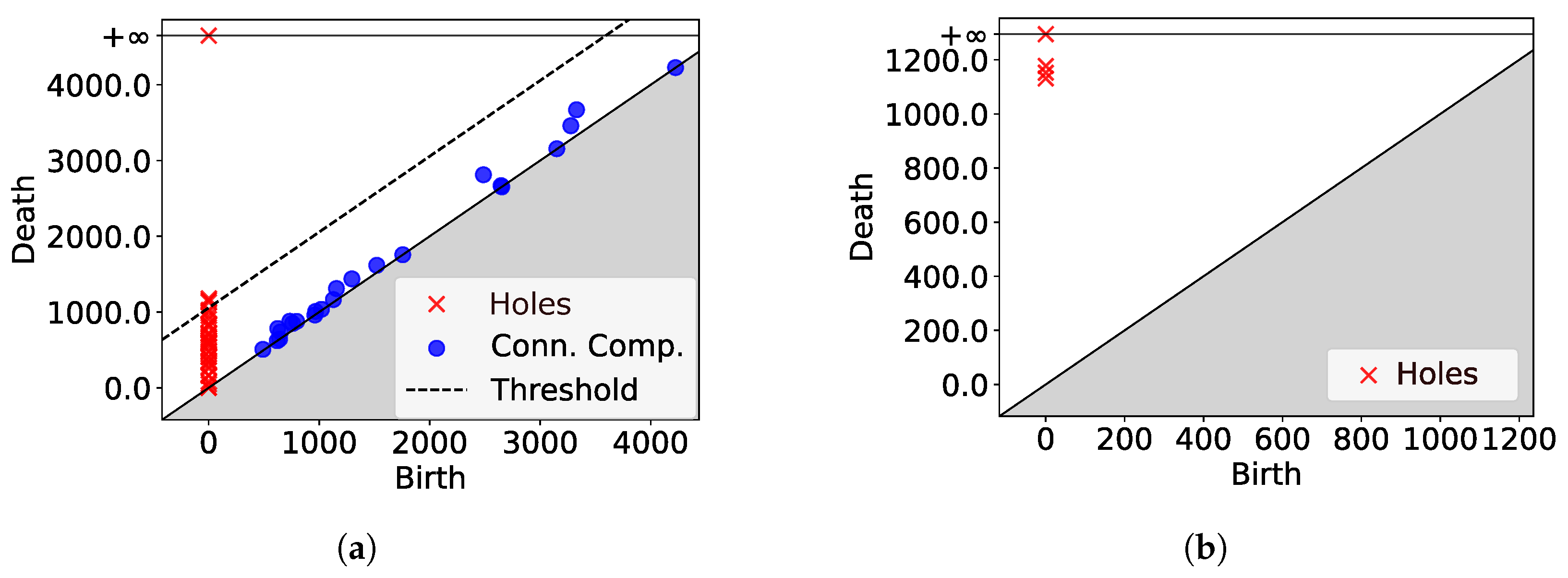
2.1.3. Topological Data Analysis (TDA) and Persistence Homology

This is a new field with many applications in computational geometry and data analysis. It uses the topology and geometry of the data to obtain information about their structure and perform qualitative and quantitative analyses [41]. TDA captures complex topological structures within data that are represented as a point cloud. A point cloud refers to a collection of distinct data points distributed in an n-dimensional space. The concept of a persistent homology involves measuring topological features at multiple spatial scales. This is achieved by studying the evolution of different topological features such as the number of holes in the object representation (topological space) of the point cloud. The Rips complex [42] and Cech complex [43] are two such well-known topological space construction methods. Both these approaches consider neighborhoods of a given radius around points and merge all the points within the neighborhood.

The persistence diagram (PD) provides a way to study a topological space by depicting the birth and death of topological features, such as connected components or holes, as we increase the radius. It provides a nice graphical view of the topological structure of a dataset (represented as an n-dimensional point cloud). It is used for various purposes such as feature selection, pattern recognition, and shape analysis [34]. It maintains a simplex tree, which is a flexible and efficient data structure to represent and store filtered data. Figure 3 demonstrates the creation of a PD for a given cluster using the Rips complex as the topological space creation method [44]. Figure 3a is the point cloud representation of the cluster, Figure 3b represents the Rips complex of the points in the cluster, and Figure 3c is the final PD of the cluster. The x and y axes represent time units, where it is assumed that the radius increases linearly with time. A point at $(x_1,y_1)$ means that a specific feature (hole or connected component) was visible for the first time (born) at time $x_1$ and stopped being visible (died) at time $y_1$.

2.2. Simulation of Urban Mobility (SUMO): Traffic Simulator

SUMO is an open-source, microscopic traffic simulation software widely used to generate traffic distributions in an urban area [45]. It can simulate various transport-related entities such as public transport, vehicles, and traffic control mechanisms. We can model traffic, build networks, control traffic, conduct environmental analyses, and visualize real-time simulated traffic data. It is widely used in academia and industry. It can easily be integrated with other tools for various applications. Figure 4 represents the traffic simulated on the map of a region in Berlin, Germany. The points shown in this figure depict the road network of the city.

2.3. JAYA Algorithm

The JAYA algorithm is a population-based metaheuristic algorithm recently proposed by Rao et al. [46]. The algorithm combines the characteristics of evolutionary algorithms and swarm intelligence. It is inspired by the survival-of-the-fittest principle of natural selection. The algorithm uses very few hyperparameters. Hence, it does not require extensive tuning.

3. Problem Formulation

We shall describe a generic charging station placement problem [2,3,4,5,8] in this section. A few definitions follow. Candidate charging stations (CCSs) are all the potential locations for deploying CSs on a given city map. We define a DP (demand point) as a location where EV charging is in significant demand. Let us define ${\mathcal{S}}_{DP}$ to be the set of all demand points, ${\mathcal{S}}_{CS}$ to be the set of all charging stations, and ${\mathcal{S}}_{CCS}$ to be the set of all candidate charging stations. Clearly, ${\mathcal{S}}_{CS}\subseteq {\mathcal{S}}_{CCS}$. $N_{dp}=\left|{\mathcal{S}}_{DP}\right|$ is the total number of DPs, $N_{cs}=\left|{\mathcal{S}}_{CS}\right|$ is the total number of charging stations, and $N_{ccs}=\left|{\mathcal{S}}_{CCS}\right|$ is the total number of candidate charging stations.

We can now define a shortest Euclidean distance matrix $\mathbf{D}$ of dimension $N_{dp}\times N_{ccs}$, where $\mathbf{D}\left[i\right]\left[j\right]$ denotes the shortest Euclidean distance between the $i^{th}$ DP and the $j^{th}$ CCS. Let the maximum distance that an EV user can travel to reach a charging station be $\tau$. This is known as the reachability distance. As a result, we must ensure that after traveling a distance of $\tau$, the EV user definitely has access to a CS.

The total number of CSs that can be deployed in a city is subject to a budget. Let $\beta$ represent the maximum number of CSs that can be deployed in a city. Hence, the actual number of deployed CSs ($N_{cs}$) should always be less than the maximum budget ($\beta$) for CSs, i.e., $N_{cs}$ ≤ $\beta$. Let $\mathbf{S}$ be the supply matrix of dimension $N_{dp}\times N_{ccs}$, which represents the allocation (mapping) of a CS to a DP. $\mathbf{S}\left[i\right]\left[j\right]$ = 1 implies that the $j^{th}$ CCS is allocated to the $i^{th}$ DP, otherwise $\mathbf{S}\left[i\right]\left[j\right]$ is 0. Let $\mathcal{O}$ be a binary array with $N_{ccs}$ elements which indicates whether a CCS is finally chosen to be a CS or not. $\mathcal{O}\left[i\right]$ = 1 implies that the $i^{th}$ CCS is considered as a CS, otherwise it is not considered to be a CS.

The aim is to ensure an optimal placement of the CSs across the city. To solve this problem, we minimize the cost, which can be represented as an objective function ${\sum }_{i=1}^{N_{dp}}{\sum }_{j=1}^{N_{ccs}}\mathbf{D}\left[i\right]\left[j\right]\times \mathbf{S}\left[i\right]\left[j\right]$. This is the sum of the total distance that all EV users have to travel (assuming there are the same number of users at each demand point). The overall mathematical formulation of the problem is shown below.

$$\begin{array}{c}\hfill \begin{array}{c}\hfill Minimize\sum _{i=1}^{N_{dp}}\sum _{j=1}^{N_{ccs}}\mathbf{D}\left[i\right]\left[j\right]\times \mathbf{S}\left[i\right]\left[j\right]⊳\mathrm{Overall}\mathrm{distance}\end{array}\end{array}$$

(1a)

$$\begin{array}{c}\mathrm{Subject}\mathrm{to}:\hfill \\ \hfill \begin{array}{c}\hfill \hspace{1em}\hspace{1em}\hspace{1em}\hspace{1em}\sum _{j=1}^{N_{ccs}}\mathbf{D}\left[i\right]\left[j\right]\times \mathbf{S}\left[i\right]\left[j\right]\le \tau ,\forall i\in \{1\dots N_{dp}\}⊳\mathrm{Reachability}\end{array}\end{array}$$

(1b)

$$\begin{array}{c}\hfill \begin{array}{c}\hfill \sum _{j=1}^{N_{ccs}}\mathbf{S}\left[i\right]\left[j\right]=1,\forall i\in \{1\dots N_{dp}\}⊳\mathrm{One}\mathrm{CS}\mathrm{connected}\mathrm{to}\mathrm{one}\mathrm{DP}\end{array}\end{array}$$

(1c)

$$\begin{array}{c}\hfill \begin{array}{c}\hfill \mathbf{S}\left[i\right]\left[j\right]\le \mathcal{O}\left[j\right],\forall i\in \{1\dots N_{dp}\},j\in \{1\dots N_{ccs}\}⊳\mathrm{Associate}\mathrm{only}\mathrm{if}\mathrm{the}\mathrm{CCS}\mathrm{is}\mathrm{a}\mathrm{CS}\end{array}\end{array}$$

(1d)

$$\begin{array}{c}\hfill \begin{array}{c}\hfill \sum _{i=1}^{N_{ccs}}\mathcal{O}\left[i\right]\le \beta ⊳\mathrm{Budget}\mathrm{condition}\end{array}\end{array}$$

(1e)

Constraint (1b) ensures that all the DPs must be at most $\tau$ units of distance away from a placed CS. Constraint (1c) states that $\forall DP$, a CS must be allocated to it. This constraint is very helpful in distributing the demand of DPs efficiently. Constraint (1d) ensures that the allocated CS must be chosen as a CS (sanity check). Finally, constraint (1e) states that the number of CSs must be less than or equal to the budget $\beta$. This model is similar to the one proposed by Kulkarni et al. [47] and is similar to the models in many more references [1,7,9,10,11,12].

Our primary constraints helped us to identify the exact location to place the CSs. But, just placing the CSs does not solve our woes. We need to take care of other electrical constraints such as constraint (2) (described in Section 3.1), and we need to be sure that the areas with high traffic (most visited roads) are handled well. We establish that if a CS is located in an area with high traffic density, it would require additional chargers to serve the customers. Basically, a charger is a power supply device that supplies power for recharging an EV. A CS can have multiple chargers. These chargers reflects the size and capacity of a CS.

In order to simplify the underlying problem and enhance the performance of the method, we consider all these constraints as additional constraints.

It is a standard practice to divide the problem into two parts: a solution that satisfies the primary constraints, and then modifications to the solution based on additional constraints: traffic conditions, capacities of charging stations (issue of inductive and capacitive loads), electrical regulations, and the importance of the area as additional constraints. The additional constraints mostly affect the internal working of the charging station [48,49].

3.1. Additional Constraints

Let us incorporate additional information about the traffic, electrical load, and queuing time in the model. The overall electrical load is dependent upon multiple aspects, including but not restricted to the charging pattern (fast charging), the popularity of the charging stations (public charging stations, workplace charging stations), the power efficiency of the chargers, and the charging capacity of the electric vehicles. EV chargers are high-frequency electronic converters that transform the AC supply into a DC supply to charge an EV. These converters impose a load of a nonlinear nature that has an adverse impact on the performance of the power grid as it introduces harmonics into the system [50]. Additionally, the process of charging electric vehicles (EVs) results in a quick and impulsive increase in the load on the charging infrastructure, hence causing voltage instability issues. Thus, balancing the load among the CSs is crucial.

To achieve this, first, we need to define the number of chargers in a CS. So, let the matrix $\mathbf{K}$ of size $N_{cs}\times N_a$ represent the allocation of a charger to a CS, where $N_a$ is the total number of chargers. $\mathbf{K}\left[i\right]\left[j\right]$ = 1 means that the $j^{th}$ charger is allocated to the $i^{th}$ CS, otherwise $\mathbf{K}\left[i\right]\left[j\right]$ is 0. Using $\mathbf{K}$, we define $a_i={\sum }_{j=1}^{N_a}\mathbf{K}\left[i\right]\left[j\right]$ as the number of chargers at the $i^{th}$ charging station.

Let us add some electrical constraints to the model [12]. In the real world, CSs will present themselves as large electrical loads. By adding these constraints, we can distribute the electrical load more efficiently across phases and across CSs. We define an array L of size $N_{cs}$, where $L\left[i\right]$ denotes the total load placed on the $i^{th}$ CS. It is a deciding factor in estimating the largest amount of load that can be placed on a CS such that it still maintains harmonic in-line currents, phase balance, and voltage deviations (within the limit). Additionally, each CS should contain at least one charger (sanity check). The following equation (constraint (2)) highlights that the chargers in a CS should not be overloaded, and still contain at least one charger.

$$\begin{array}{c}\hfill \begin{array}{c}\hfill 1\le a_i\le \frac{L\left[i\right]}{{\rho }_{ev}}⊳\mathrm{Chargers}\mathrm{in}\mathrm{a}\mathrm{CS}\mathrm{must}\mathrm{not}\mathrm{be}\mathrm{overloaded}\end{array}\end{array}$$

(2)

Here, ${\rho }_{ev}$ denotes the charging power rating of an EV. Constraint (2) is used to tackle the load imbalance problem across CSs, as the maximum load of a CS must be less than the overloading factor L [21]. The chargers are also allotted a budget (${\beta }_a$). Constraint (3) highlights the fact that the total number of chargers in a region should not exceed the budget for that region (${\beta }_a$). This will ensure that there are no local hotspots, and that the power requirement of a CS never exceeds the substation’s capacity and power quality is maintained.

$$\sum _{i=1}^{N_{cs}}{a}_i\le {\beta }_a⊳\mathrm{Total}\mathrm{budget}\mathrm{of}\mathrm{chargers}$$

(3)

Next, we define the queuing time [51,52] as the time spent waiting in a queue to charge the EV. This depends on several factors such as the traffic at a CS, the charging time for each EV, and the number of chargers available at a CS [51]. We use a queuing model to model the traffic and the queuing time across the city; this is a popular model that has been used in a lot of prior work. It was proposed by Zhu et al. [51].

The queuing time at a CS increases proportionally to the increase in demand and traffic, whereas an increase in the number of chargers at the said station will reduce the queuing time, as presented in Equation (4a). This model is similar to the one proposed by Zhu et al. [51].

$$\begin{array}{c}\hfill \begin{array}{c}\hfill Q_i=\frac{a_i{\left({\eta }_i{a}_i\right)}^{a_i+1}{P}_{0i}}{{\lambda }_i{a}_i!{(a_i-a_i{\eta }_i)}^2}⊳\mathrm{Queuing}\mathrm{time}\mathrm{at}\mathrm{the}{i}^{th}\mathrm{CS}\end{array}\end{array}$$

(4a)

$$\begin{array}{c}\hfill \begin{array}{c}\hfill {\lambda }_i=\frac{{\sum }_{j=1}^{\mathrm{x}}{\mathcal{X}}_i\left[j\right]}{t_c}⊳\mathrm{Traffic}\mathrm{flow}\mathrm{rate}\mathrm{around}\mathrm{the}{i}^{th}\mathrm{CS}\end{array}\end{array}$$

(4b)

$$\begin{array}{c}\hfill \begin{array}{c}\hfill P_{0i}={\left[\left(\sum _{j=0}^{a_i-1}\frac{{\left({\eta }_i{a}_i\right)}^j}{j!}\right)+\frac{{\left({\eta }_i{a}_i\right)}^{a_i}\left(a_i\right)}{a_i!(a_i-a_i{\eta }_i)}\right]}^{-1}⊳\mathrm{Probability}\mathrm{of}\mathrm{finding}\mathrm{an}\mathrm{idle}\mathrm{charger}\mathrm{at}\mathrm{the}{i}^{th}\mathrm{CS}\end{array}\end{array}$$

(4c)

$$\begin{array}{c}\hfill \begin{array}{c}\hfill {\eta }_i=\frac{{\lambda }_i}{\mu a_i}⊳\mathrm{Chargers}’\mathrm{utilization}\mathrm{at}\mathrm{the}{i}^{th}\mathrm{CS}\end{array}\end{array}$$

(4d)

$$\begin{array}{c}\hfill \begin{array}{c}\hfill \mu =\frac{1}{t_s}⊳\mathrm{Service}\mathrm{time}\mathrm{of}\mathrm{a}\mathrm{charger}\end{array}\end{array}$$

(4e)

Here, ${\lambda }_i$ denotes the EV traffic at the $i^{th}$ CS (Equation (4b)) and $t_c$ denotes the time duration during which the traffic was monitored. We estimate the traffic at a CS by simulating the traffic flow using the SUMO traffic simulator. Here, we make the reasonable assumption that the traffic in a CS is dependent on the EV traffic within the reachability distance. ${\lambda }_i$ is calculated by adding all the EV traffic of the nodes on the road that are $\tau$-reachable (within $\tau$ units of distance) from that CS. Let ${\mathcal{X}}_i$ be an array of size x, where x is the number of nodes that are $\tau$-reachable from the $i^{th}$ CS and ${\mathcal{X}}_i\left[j\right]$ denotes the traffic between the $i^{th}$ CS and the $j^{th}$ connected node.

Next, $P_{0i}$ defines the probability of finding an idle (empty) charger upon arrival at the $i^{th}$ CS, and is defined in Equation (4c), where ${\eta }_i$ represents the utilization factor of a CS, which measures the degree of utilization of the chargers (Equation (4d)). Here, $\mu$ represents the service time of a charger, which is inversely proportional to the charging time of a single charger $t_s$ (Equation (4e)).

The aim is to reduce the queuing time and minimize the total number of chargers used. Keeping this in mind, additional objective functions can be defined as follows:

$$\begin{array}{c}\hfill Minimize\sum _{i=1}^{N_{cs}}{Q}_i⊳\mathrm{Additional}\mathrm{objective}\mathrm{function}1\\ \hfill Minimize\sum _{i=1}^{N_{cs}}{a}_i⊳\mathrm{Additional}\mathrm{objective}\mathrm{function}2\end{array}$$

(5)

We can have multiple objective functions in our formulation. From a single-objective optimization problem, it will become a multi-objective optimization problem. A Pareto optimal point can be chosen subject to some overall desirability function, as is the standard practice.

Now, that the problem has been defined, we need to find a method to effectively solve it. To achieve this, we need to understand the features present in modern cities and show that their layouts are quite similar, in a topological sense. This means that they consist of a set of basic primitives, where each primitive can be arbitrarily stretched and deformed (in certain ways). This is the objective of the next section.

4. Characterization

A collection of selected nodes (CCSs) represents a city’s road network. In order to identify the topological shapes present in a city, the first aim is to select the best clustering algorithm to identify and isolate constituent topological clusters (of CCSs) from a city’s road network.

Clustering Algorithm—Identification of the Clusters in a City

We perform an extensive analysis of several state-of-the-art clustering algorithms, namely, k-means, agglomerative, and ToMATo to determine which algorithm can successfully isolate the topological clusters of CCSs present in a city. The details of the clustering algorithms are presented in Section 2.1.1. The analysis is performed on a section of Berlin, Germany, using the system configuration detailed in

Table 1. System configuration.

Hardware Settings
Chip: Apple M1	CPU cores: 8
GPU: Apple M1 8-core GPU	DRAM: 8 GB
Software Settings
Operating System: MacOS Monterrey 12.6	Python Version: 3.7
TensorFlow Version: 2.11.0	Tkinter Version: 8.6.12
Gudhi Version: 3.8.0	CVXPY Version: 1.3.1

.

We improve the computation speed of the clustering algorithms by performing random point reduction [53,54,55] (random sampling) to reduce the number of points. This is performed for all the algorithms. We empirically determined that it is possible to decrease the points by up to $75\%$ without causing much distortion to the topological shapes.

Let us consider a representative example. Figure 1a shows the input points for the clustering algorithm after performing point reduction on a section of the Berlin city. Figure 1b shows the outcome of k-means clustering with 10 clusters ($k=10$). Due to the fact that k-means assumes that each cluster has the same size and is susceptible to noise, it is quite incapable of isolating the topological shapes.

Figure 1c shows the outcome of agglomerative clustering with 10 clusters. We observe that the clusters that are generated by the algorithm are relatively similar to the ones generated by k-means clustering. They also fail to isolate the topological shapes. Figure 1d shows the outcome of ToMATo with radius $r=80$. The algorithm generates clusters by connecting all the nodes within a radius of 80 m. It can isolate the majority of the topological shapes as it considers both the highly dense and less dense areas. We conclude that the clusters generated by ToMATo can successfully isolate a majority of the shapes. In our experiments, this observation is found to hold across all big cities (our dataset). Therefore, this is the most desirable clustering algorithm for identifying the constituent topological shapes of a city.

Next, we take a look at the proposed scheme and how it uses the clustering algorithm.

5. Material and Methods

5.1. Overview of the Scheme

The primary objective of this work (problem 1) is to identify the locations of CSs based on a set of primary constraints (budget, reachability radius, demand points). Similar to prior work [48,49,56], we address an additional objective (problem 2) of distributing the chargers among the CSs such that no additional constraints (traffic, electrical regulations, queuing time) are violated.

Problem 1: Figure 5 shows that the primary objective is achieved using the proposed PC-ILP algorithm by using a hierarchical decomposition method. In this method, the city map (represented as a set of CCSs) is decomposed into clusters of CCSs using a topological clustering algorithm. Next, a CNN is used to identify the geometric shape of each cluster.

We study topological shapes (clusters of CCSs) present in 50 of the largest cities in the world, and based on our findings, we argue that a few basic shapes can be used to capture the topological structures of most cities. This conclusion is supported by the fact that a small number of 2D simplexes (a line, a circle, a mesh, a star, and a concentric circle) can be used to define any topological shape of interest in a modern city [57]. We present a pictorial representation of all the 2D simplexes in Figure 6. Our experiments support this assumption.

These clusters are seen as small subproblems and we use a database of precomputed solutions to solve these subproblems. The database comprises optimal solutions for various shapes (clusters of CCSs) over a spectrum of parameters including the number of DPs, budget, and reachability distance, as shown in

Table 2. Primary parameters of the problem.

Parameter	Description
${\mathcal{S}}_{CCS}$	The CCSs depict the potential charging stations across the city.
$\tau$	The reachability distance is the maximum distance an EV user needs to travel from a DP.
$\beta$	The budget represents the maximum possible number of CSs in a city.
${\mathcal{S}}_{DP}$	The demand points correspond to the points in the city that demand EV charging.

. During the runtime, a user only needs to look at the database to obtain a solution for each shape. However, the final solution that has been obtained from the database may not be feasible. Such infeasible solutions are fixed using a surrogate function (details to follow).

Problem 2: Then, the repaired/feasible solution from PC-ILP is sent to the second stage—a small ILP optimization problem. This considers a few of the additional parameters (traffic, queuing time, and electrical regulations). The reason for this is that the traffic patterns within a city can exhibit severe variations. Consequently, attempting to create a database capable of accommodating all of these combinations would not be feasible. The queuing time also depends on the traffic in a CS, so it is also considered as an additional parameter. Additionally, the electrical regulations also directly influence the number of chargers in a given CS. Therefore, all of these factors are categorized as additional parameters, which have a direct impact on the number of chargers in each CS. This ILP stage (which is a much smaller problem) finds the optimal number of chargers that need to be placed at each CS. This stage is needed for flexibility. Modern EV placement problems can have a lot of constraints and objective functions (soft and hard). Hence, a two-stage approach suits us well.

5.2. Placement of Charging Stations (Primary Objective)

A high-level diagram of the proposed scheme is shown in Figure 7. The algorithm is divided into six major components: ❶ Precomputation of the ILP solutions for various basic shapes. These solutions are stored in a database. ❷ Identification of the potential charging point locations (CCSs) in a city. ❸ Partitioning of the city map into distinct clusters of CCSs using ToMATo. ❹ Basic shape identification of the clusters using a CNN. ❺ Finding the most appropriate match in the database for the identified shape. ❻ Estimation of the final solution based on the matching solution from the database. Algorithm 1 describes our proposed scheme. We also show a glossary of the symbols in

Table 3. A nomenclature of the symbols.

Symbol	Definition	Symbol	Definition
$N_{ccs}$	Number of CCSs	$\mathbf{D}$	The distance matrix between DPs and CCSs
$N_{dp}$	Number of DPs	$\mathcal{M}$	Mapping between cluster and DPs
$\tau$	Reachability distance	$\beta$	Budget (max allowed CSs)
$N_{cs}$	Total number of CSs	$\mathbf{S}$	The supply matrix (DP-CS allocation)
$\mathcal{O}\left[N_{ccs}\right]$	Boolean array that indicates whether a CCS is a CS	$\mathcal{P}$	A set of basic shapes and DP distribution
$\mathcal{C}$	A set of clusters	$\mathcal{DB}$	Precomputed database
S	The shape of a cluster	$SimS$	A similar shape retrieved from the database
$\left|X\right|$	Size of the set X	$\{x,y\}$	Concatenate x and y

.

Algorithm 1: PC-ILP (online stage)

5.2.1. Create Database of Precomputed Solutions (Offline)

The first stage is creating an exhaustive database containing solutions to the CS placement problem for a set of basic shapes. Each basic shape is represented by a set of CCSs.

• ▸ Normalization of the latitude and longitude: Each of the CCS nodes in a shape is denoted by a pair of latitude and longitude coordinates. Now, across cities, the constituent topological shapes may remain the same, but their sizes may vary significantly. Since it is not possible to store the results for all potential basic shape sizes in a database, we normalize the values of the longitudes and latitudes for different shapes. Normalizing the geographical coordinates in a large urban city to store a scaled version of the geographical information is a well-known concept that is used in urban city planning [58,59,60,61,62]. It helps to simplify and generalize the geographic data (nodes), making them more manageable.

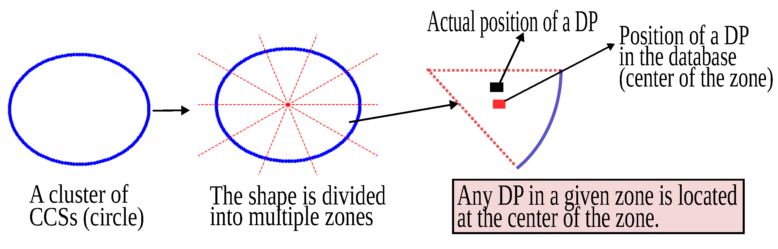
To achieve this, we normalize the location of each node, i.e., the latitude and longitude values, such that they lie in the range $[0,1]$. This is performed for a combined set of DPs and CCSs (${\mathcal{S}}_{CCS}\cup {\mathcal{S}}_{DP}$) as normalization of each set individually would distort the locations of the DPs.

We empirically estimated the size of the shapes in 50 of the largest cities in the world and observed that the maximum area of a shape among all the five basic shapes is 8.5 km${}^2$, while the minimum possible area is 1 m${}^2$. Our resolution is quite fine, even though such a granularity is almost never required. Most of the time, we can cover a roughly 3 km × 3 km section of the city in a single well-defined basic shape.

• ▸ Patterns of DP distribution in a shape: DPs denote the points at which a demand for charging exists. We place DPs manually based on the density of CCSs, the presence of public amenities like malls and hospitals, and downtown areas. To characterize the location of DPs, we subdivide all the normalized shapes into zones. If a DP falls in a zone, we assume that it is in the centroid of the zone (refer to Figure 8). This means that there is some feature of interest in the city and all the roads in the vicinity lead to it.

We ensure that our database captures all the possible locations of the DPs in a city. Let us assume that the maximum possible number of DPs associated with a shape is d and the total number of zones in a shape is z, then the total number of possible DP patterns that should be present in the database is ${\sum }_{i=0}^d{}^z{C}_i$. ${}^z{C}_i$ is the number of ways in which we can choose i elements out of z elements (number of combinations).

After successfully estimating all the possible DP distribution patterns for a given shape, we apply ILP to solve the CS placement problem for the shape and the corresponding DP distribution patterns, given a budget and a reachability radius. This generates possible sets of locations for the CSs. This procedure is conducted offline. We combine the locations of the CSs with the shape (cluster of CCSs) and the parameters (DP distribution pattern, budget, reachability radius) into one single database entry. In addition, we also compute ILP solutions for a given shape and DP distribution pattern for a range of budget and reachability radii (the range is estimated empirically) and add all the computed solutions to the database.

After creating the database, we estimate the solution for a new input map using the precomputed database. The next series of steps are all performed online.

5.2.2. Locating Potential Charging Stations in the Input Map

The first task is to identify the prospective CCSs in the input map. To identify prospective CCSs in the cities, we identify the road network of the city and place CCSs along it. We developed our in-house interactive tool $MapperCS$ that enables the filtering of the street data from a specific city map and also identifies the potential CCSs (see Section 6).

5.2.3. Clustering Algorithm

Next, we perform clustering on the CCS set to isolate the basic clusters using a topological clustering algorithm, ToMATo. It captures all the topological shapes present in a city. The computation speed of the clustering algorithm is improved by randomly reducing the number of points [53,54,55] in the CCSs using the ReducePoints function.

• ▸ Mapping DPs to clusters: In the next step, we map each DP (represented as $D{P}_i$) to its nearest cluster ${\mathcal{C}}_i\in \mathcal{C}$. A single cluster can be mapped to many DPs, creating a many-to-one mapping. To map DPs to a cluster, we first compute the convex hull for each cluster using the QuickHull algorithm [63]. We categorize the DPs into two categories based on their position relative to the convex hull. ➀ The DPs that are contained within the convex hull of a cluster ${\mathcal{C}}_i$ are automatically mapped to ${\mathcal{C}}_i$. ➁ The DPs that fall outside the convex hull of all clusters are mapped to the closest cluster ${\mathcal{C}}_i$ using the Assign function as described in Algorithm 2. Basically, the clusters are characterized by their centroids. We find the cluster closest to a DP by estimating the distance between the centroid of the cluster and the DP. We map the DP to its nearest cluster based on the minimum distance to each centroid [64].

Algorithm 2: Function $Assign(\mathcal{C},DP)$

Once we find the closest cluster (${\mathcal{C}}_j$) for a DP ($D{P}_i$), we add the DP ($D{P}_i$) to $\mathcal{M}\left[{\mathcal{C}}_j\right]$ where $\mathcal{M}$ is the demand point–cluster mapping (DCM), which stores the details of the mapping between DPs and clusters. This process is repeated until we find a mapping for every DP. After the mapping procedure is complete, we divide the total budget in proportion to the number of CCSs covered by each cluster. To achieve this, clusters ($\mathcal{C}$) are sorted in decreasing order of the cluster size. The clusters with more CCSs are allotted a greater portion of the budget ($\beta$), as described. Subsequently, we iterate over the sorted clusters $\mathcal{C}$ and process each cluster ${\mathcal{C}}_i$ individually. The next task is to identify the shape of the cluster ${\mathcal{C}}_i$.

5.2.4. Shape Identification Using a Convolutional Neural Network (CNN)

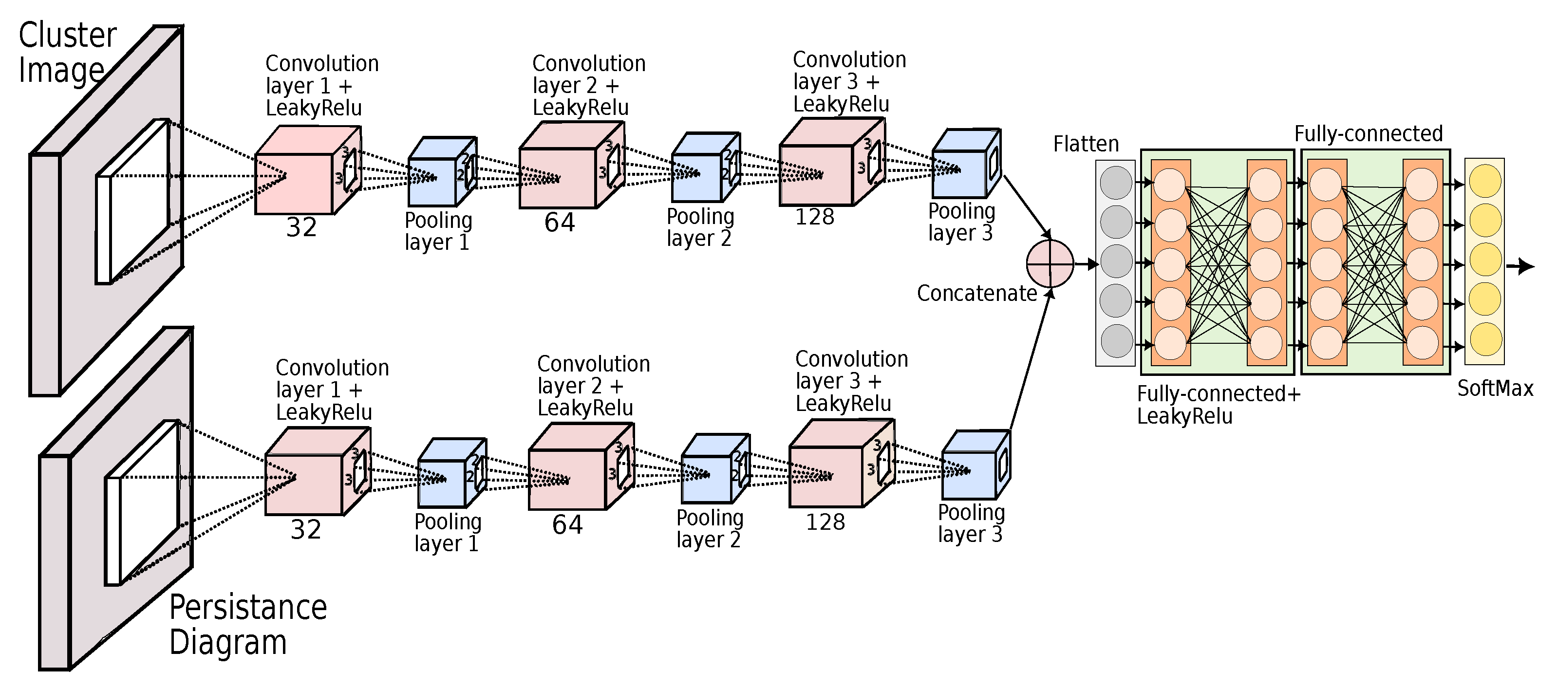
To determine the shape of a given cluster, we use a CNN model. We studied the constituent shapes of the major urban agglomerations of the world to create a realistic dataset for training and testing the CNN model. After extensive experimentation, we designed a novel CNN architecture capable of identifying shapes. The architecture is presented in Figure 9.

The input of the model is the point cloud and the PD of its MAT. The PD of the MAT of the point cloud is generated by removing holes and connected components which are less persistent by introducing a threshold, as illustrated in Figure 10. Figure 10a is a typical PD and Figure 10b is the PD of the MAT (modified PD) after thresholding. Now, let us take a deeper look at the architecture of the model.

• ▸ Model architecture: The proposed model architecture comprises two parallel CNN layers, as depicted in Figure 9. Both layers consist of an identical three-layer CNN architecture. In the three sequential convolutional layers, the number of filters increases in the sequence (32, 64, 128). Each convolutional layer is followed by a Leaky ReLU activation function and a maxpooling layer with a pool factor of $2\times 2$. Finally, we employ a regularization technique called dropout, which involves randomly deactivating the neurons within a layer. The respective dropout percentages for the three convolutional layers are $25\%$, $25\%$, and $40\%$.

The outputs of the two parallel convolutional structures are combined using a concatenate layer. Thereafter, the result of this layer is changed from a 2D matrix to a 1D vector using a flatten layer. This conversion enables the output to be processed by the fully connected layers (dense layer).

The dense layer consists of 512 neurons and a Leaky ReLU activation function, which is followed by another dropout layer that is configured to exclude 50% of the neurons. The subsequent fully connected layer has five neurons for the five basic shapes. Finally, we use the softmax activation function to predict the class of the cluster. The above-described model can identify an input shape quite accurately.

Now that we have successfully identified the shape of a cluster (IDShape function), we must query our precomputed database to discover the closest matching solution for a new input cluster.

5.2.5. Retrieval of the Precomputed Solution from the Database

The next step of PC-ILP is to identify the closest solution for a new cluster from a database of precomputed solutions using the TraverseDB function. We first need to normalize the input cluster to set it in the same scale as the clusters in the database (refer to Section 5.2.1). For the solutions of any two clusters to be broadly similar, they must be ➀ of the same shape and ➁ have similarly placed DPs with respect to the shape of the CCSs. The similarity in the DPs can be measured by finding out the zone of each demand point with respect to the shape. If the DPs in both the clusters fall in the same zones, then we can argue that the DP distribution is similar.

Next, we determine whether the solutions presented in the closest matching shape(s) are within the input budget. We choose the solution with the lowest budget (represented as $SimS$). This enables us to maintain a contingency budget that can be utilized in the event of constraint violations. A closest match will always be found in the database as we know that the database is exhaustive (as described in Section 5.2.1). Algorithm 3 describes this process in further detail.

Algorithm 3: Function $TraverseDB(S,{\mathcal{C}}_i,\mathcal{M},\mathcal{DB},b)$

5.2.6. Mapping the Precomputed Solution

The database provides the positions for the optimal locations of the CSs for the closest matching cluster ($SimS$) with the least possible budget. To apply the solution of $SimS$ to the input cluster ${\mathcal{C}}_i$, we need to relocate the CS in $SimS$ with respect to the CCSs in the input cluster. To achieve this, we find a CCS in our input cluster for each CS in $SimS$ which is within the distance threshold of T from the said CS. In the event that no such CCS satisfies this constraint, we select the one which is closest to the CS. We have empirically estimated that we can set T to be 0.1 units (where the points are normalized to the [0–1] range). Once this is complete, we denormalize the $CS$s to obtain the final solution. Algorithm 4 describes this process in detail.

Figure 11 shows a graphical illustration of the ApplySolution function. Figure 11a represents the input cluster ${\mathcal{C}}_i$, and its closest matching solution from our database $SimS$ is shown in Figure 11b. Next, we try to find the closest CCS ($CC{S}_{{\mathcal{C}}_i}$) in the input cluster for each charging station ($C{S}_S$) in $SimS$—this is shown in Figure 11c. The final solution is presented in Figure 11d.

Algorithm 4: Function $ApplySolution(SimS,{\mathcal{C}}_i,\mathcal{M},T)$

5.3. Repairing an Infeasible Solution

As with any other hierarchical solution, we must check that the assembled solution satisfies all the constraints of the original problem [28]. We observe that three of our four constraints cannot be violated due to the design of PC-ILP—each DP is associated with the CS placed closest to it. So, constraint (1c) is never violated. To ensure that constraint (1d) is not violated, we make sure that when applying the solution of $SimS$ to ${\mathcal{C}}_i$, the CSs placed for ${\mathcal{C}}_i$ are CCSs, as illustrated in Algorithm 4. We also divide the provided budget across the various shapes in order to ensure that constraint (1e) is not violated. Subsequently, a match for each cluster for a given budget is located in our database.

This leaves the reachability constraint, which may be violated, resulting in an infeasible solution. The solution to this problem is to maintain a contingency budget for use in the event of a constraint violation. This enables us to repair the infeasible solution by adding additional CSs for the demand points where a constraint violation is detected without affecting the pre-existing locations of the CSs. This simplifies the problem, allowing for a fast estimation of the feasible solution.

The initial phase is the verification step, in which we determine whether or not a constraint has been violated in the original solution. To determine this, we map all DPs within a reachability distance from a CS. This is performed for all CSs. Next, we determine if any DPs are left unmapped, which indicates that the reachability constraint has been violated (refer to Algorithm 5).

To address this issue, we solve the original optimization problem with a $15\%$ budget reduction, allowing us to use the remaining budget to fix the possibly infeasible solution. This is the surrogate optimization problem, where we use the PC-ILP algorithm, albeit with a reduced budget. First, we query the database with the unmapped DPs and a portion of the remaining budget (using the TraverseDB function). The function returns the closest matching shape for the given set of unmapped DPs and CCSs (details in Section 5.2.5). Then, we apply the solution to the matching shape using the ApplySolution function, which returns the optimal placement of the CSs for the given unmapped DPs. We recheck whether or not all the DPs are mapped using the obtained solution within the given budget. If they are not mapped, the entire procedure is repeated with a slightly increased budget.

Algorithm 5: Function $Repair(\mathcal{CS},\mathcal{DP},{\beta }_0,\mathcal{M},{\mathcal{C}}_i,S,b)$

If a feasible solution is found, to arrive at the final repaired solution we combine both the initial infeasible solution and the surrogate solution for the DPs with constraint violations. The infeasible solution consists of the locations of CSs (old CSs) that served a subset of DPs. Sadly, some DPs were left unmapped, and we used the surrogate function to add new CSs to serve those DPs using the extra budget. The final solution is essentially a union of the locations of both the sets of charging stations (new CSs and old CSs). In cases where the entire budget has been spent and no solution has been found, a solution to the problem is deemed to be impossible.

5.4. Chargers at Each Charging Station (Additional Objective)

Once a solution for the primary objective is obtained from our database, we proceed to solve an ILP problem in order to integrate the additional constraints into the estimated solution. We have referred to this as Problem 2. Our experimental observations indicate that the proposed approach has the capability to include a wide variety of additional constraints and objective functions. Nevertheless, the present version of the work presents a proof of concept by considering only the additional electrical constraints, queuing time, and traffic information. Equation (2) (see Section 3.1) introduces the concept of adding multiple chargers at each charging station, which can easily be found by solving an ILP problem. Note that the size of this problem is much smaller than our original problem, where our solution space was much larger. Here, we just have to determine the capacity (in terms of the number of chargers) of each CCS.

For our experiments, we formulate an ILP, which is in line with the equations shown in Section 3.1. The ILP problem returns the optimal number of chargers at each location (CS). We observe that the execution time for these ILPs is very small as compared to the ILP for Problem 1, due to the fact that its search space is much lower.

6. Results and Discussion

In this section, we shall discuss the evaluation methodologies that are used to compare PC-ILP to other state-of-the-art algorithms. In addition, we characterize the effect of different shapes on the performance of the solution obtained by PC-ILP for various cities.

6.1. Setup

The details of the system setup along with all the software and hardware configurations are shown in Table 1. We have developed an in-house tool named MapperCS (map-based tool using persistence homology for charging station placement), which runs on MacOS, Windows, and Ubuntu. The tool has an interactive map in the center of the screen with two side panes. MapperCS takes map data from OpenStreetMaps [35] using the overpass [65] API, filters out many details, and retains the street data, which are used to create the CCSs via a manual annotation process. Figure 12 shows a screenshot of the MapperCS tool. This highly interactive tool is designed to perform many operations on the city map using two interactive side panes. The users can not only annotate the DPs and potential CSs, but they can also perform more complex operations, such as clustering the CCSs, and run an ILP for a given set of constraints.

• ▸ Benchmarks: We consider the top 50 cities by population (source: [66]). We focus on the areas that have a high population density in the cities (35–387 km${}^2$). The details are shown in

  Table 4. The list of cities considered in our work.

  City, Country	Area (km${}^2$)	City, Country	Area (km${}^2$)	City, Country	Area (km${}^2$)
  New York, USA	386.79	Lima, Peru	241.31	Lahore, Pakistan	160.17
  Paris, France	102.34	Xian, China	220.28	Mumbai, India	291.42
  Karachi, Pakistan	153.01	Beijing, China	207.69	Moscow, Russia	128.10
  Rio de Janeiro, Brazil	171.39	Shanghai, China	157.75	Bangalore, India	125.20
  Lagos, Nigeria	165.09	Seoul, South Korea	166.19	Ahmedabad, India	147.39
  Hyderabad, India	276.80	Manila, Philippines	151.15	Chicago, USA	139.47
  Bogota, Colombia	205.81	Chennai, India	127.07	Delhi, India	257.32
  Tokyo, Japan	169.75	Sao Paulo, Brazil	240.79	Hangzhou, China	162.14
  Tianjin, China	114.95	Istanbul, Turkey	270.62	Nanjing, China	300.42
  Ho Chi Minh, Vietnam	179.39	Kinshasa, Congo	153.25	Cairo, Egypt	170.04
  Madrid, Spain	173.26	Chongqing, China	352.70	Osaka, Japan	111.54
  Jakarta, Indonesia	183.40	Kolkata, India	150.39	Chengdu, China	170.70
  Buenos Aires, Argentina	158.54	Los Angeles, USA	177.53	Dhaka, Bangladesh	185.52
  Luanda, Angola	216.53	Kuala Lumpur, Malaysia	287.39	Tehran, Iran	128.08
  London, UK	106.80	Nagoya, Japan	103.43	Hong Kong, China	316.96
  Shenzhen, China	140.79	Guangzhou, China	132.14	Mexico city, Mexico	192.33
  Wuhan, China	198.08	Bangkok, Thailand	183.51	Berlin, Germany	35.80

  . We can make some broad observations based on the maps of the cities (also visualized using our MapperCS tool). We observe that American cities have historically been laid out as grids (meshes), whereas European towns have predominantly adopted a radial organization (all the arterial roads are oriented towards the center of the city). We show two examples in Figure 13 for sections of downtown Paris and New York.
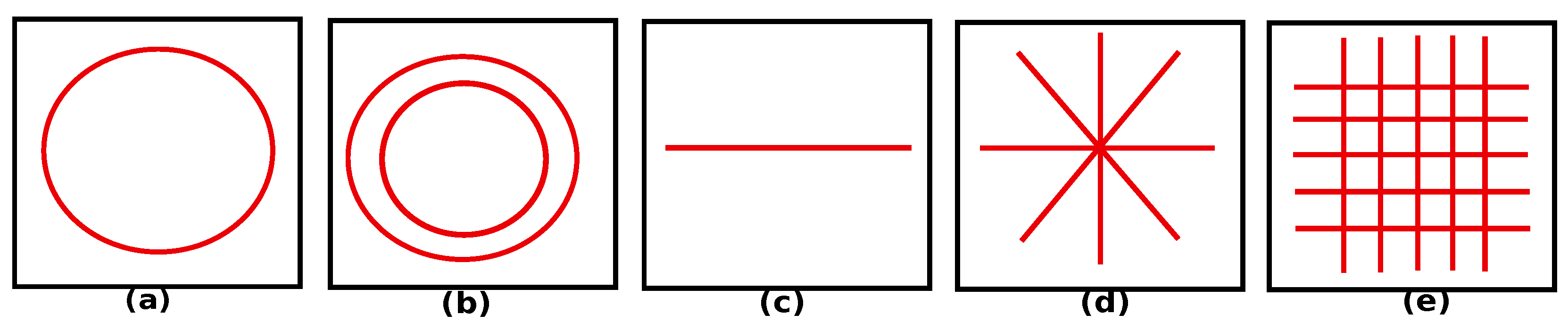
• ▸ Dataset for the CNN-based algorithm: The shapes of the clusters of CCSs are identified using a CNN model (see Section 5.2.4). The training dataset contains clusters that can be classified into five basic shapes, namely, circle, mesh, star, line, and concentric circle. Each cluster is defined by its point cloud representation and the PD of its MAT. We trained our model using synthetic data, because in this case we can generate as much as synthetic data as we want (we are not limited by the training set size or real-world constraints regarding the availability of data). For instance, if we want to generate synthetic data for a star, then we lay a random number of points out as a star, and then perturb them randomly. In this way, we can generate a lot of training examples for a given topology. The same approach can be repeated for other topologies and we can continue training our model. Note that there is no need for manual annotation here because we already know which basic shape a given point cloud corresponds to. We used the point clouds (CCS locations) in the 50 cities as test cases.

  Table 5. Shapes found in our dataset comprising 50 cities.

  Shape	Data Points
  Circle	3600
  Line	2889
  Star	2189
  Concentric circle	1248
  Mesh	203

  shows the number of shapes found across our dataset of 50 cities.

6.2. Parameters for the Creation of the Precomputed Database

6.2.1. Number of Zones in Each Shape

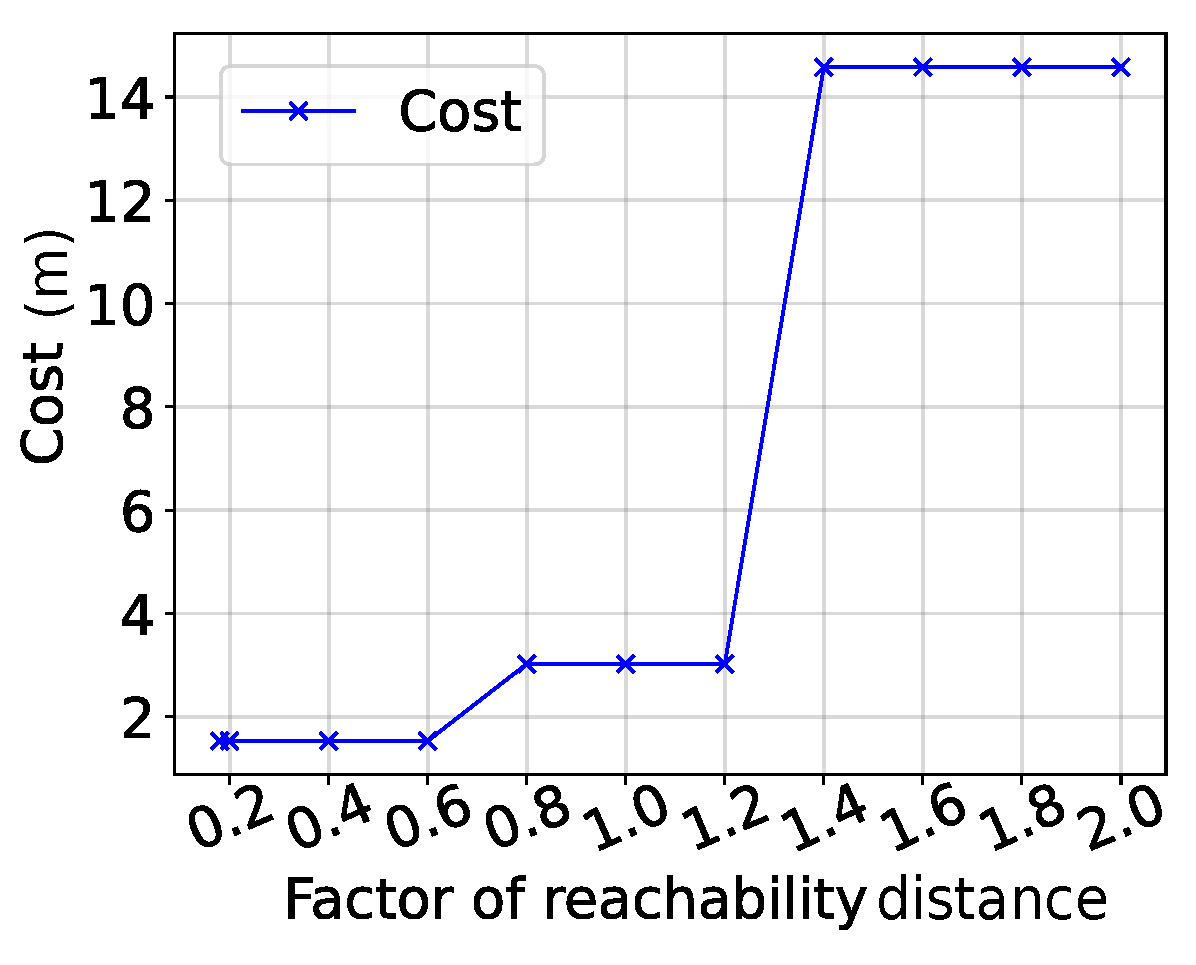
The number of zones within a shape affects the total number of DP distribution patterns, which in turn influences the size of the database. We perform extensive experiments to find the total number of zones in each basic shape. We estimate the cost (see Equation (1a)) using ILP for two scenarios: (a) when the DP is located in the centroid of the zone; and (b) when the DP is located anywhere else in the zone.

We considered 250 randomly generated patterns for DPs (for a given number of CCSs, budgets, and reachability radii) and computed the difference in the costs for the two scenarios for a given number of zones. This experiment was repeated by increasing the number of zones in a shape. The results for the average cost difference for different shapes are shown in Figure 14. We observe that after a certain limit, the difference in the cost reduces and reaches a saturation point; the knee point is used to set the number of zones in a shape. We conclude that we should divide the circles into 20 zones, whereas stars, meshes, and lines should be divided into 16 zones, and finally, concentric circles should be divided into 24 zones. In our experiments, these were found to be the optimal values.

6.2.2. Reachability Distance ($\tau$)

The reachability distance ($\tau$) denotes the maximum distance that an EV user needs to travel from the DP to the nearest CS to charge the EV. We performed exhaustive experimentation to analyze the effect of the reachability distance on the cost of the solution. For each shape, we first computed the ILP solution with $\tau ={\tau }_{input}$, where ${\tau }_{input}$ is the input reachability distance. After this, we computed the ILP with $\tau \in [0.2{\tau }_{input},2{\tau }_{input}]$. Figure 15 shows the variation in the cost function with the reachability distance for a circle with a constant budget of four CSs, 117 CCSs, and three DPs. We observe that after a certain value of the reachability distance, the cost of the solution remains nearly constant. A similar observation is highlighted by Gopalakrishnan et al. [67]. We ensure that the database has solutions for all potential values of the reachability distance prior to the saturation point for different combinations of the DP distribution and the budget.

6.2.3. Budget ($\beta$)

We allocate a budget to a city that represents the total number of CSs that can be placed in the city. However, we know that placing a CS without demand wastes resources. Therefore, the budget and the demand points are directly related. In the worst-case scenario, each DP will have its own CS. Therefore, the total number of CSs (or budget) can never exceed the number of DPs. This establishes an upper limit on the budget.

Additionally, we observe that our clusters are created in such a way that a cluster can have a maximum of three demand points. This is because big cities may consist of many small-sized clusters as the ToMATo-clustering generates many small clusters, as shown in Section 5.2.3, and demand points will be divided across these small clusters. We experimentally validated that a cluster with more than three DPs is quite unlikely. We ensure that our database contains all possible solutions within the specified budget range for each cluster.

6.3. Performance Analysis

In this section, we evaluate our schemes for a set of micro- and macrobenchmarks. We consider two metrics for evaluation: ➀ the execution time of each algorithm and ➁ the cost of the solution provided by the algorithm (see Equation (1a)).

6.3.1. Microbenchmarks

To evaluate the efficiency of PC-ILP, we compare it against the standard ILP approach [47] (timeout set to 1 h), the state-of-the-art lazy greedy with efficient gain (LGEG) algorithm [8], and a fast metaheuristic JAYA algorithm [5], which uses a genetic algorithm. As the ILP algorithm is time- and memory-intensive, we compare the algorithms on a microbenchmark, which is a section of Berlin, Germany. We select an area of 32.50 km${}^2$ which contains approximately 4100 CCSs. We reduce the number of CCSs in this area to 2500 due to the memory constraints of the ILP. We choose 30 DPs and a budget of 35 CSs. The DPs are generated uniformly at random, similar to Lam et al. [68]. Additionally, in order to run the ILP with the given setup, we set an upper bound on the execution time to avoid memory overflow. After exhaustive experimentation, we selected an upper bound of 3600 s.

• ▸ Cost vs. budget: We evaluate the performance of the algorithms by gradually increasing the allocated budget while keeping the CCSs and DPs fixed.

Figure 16 compares the solutions provided by the various algorithms against the allocated budget. Figure 16a shows that the cost of the solution provided by JAYA and LGEG is worse than both ILP and PC-ILP. Specifically, PC-ILP outperforms LGEG by 38.87% and JAYA by 5.09 times with respect to the solution cost, which is expected as LGEG is not operating exhaustively on the CCSs and DPs, and genetic algorithms are known to scale poorly against complexity due to the exponential increase in the size of the search space.

Upon closer inspection, we see that the solutions provided by PC-ILP are marginally better than the ILP solutions. Figure 16b shows that PC-ILP and LGEG are faster than standard ILP. This is expected as the ILP is more time- and memory-intensive than both LGEG and PC-ILP. We also observe that PC-ILP provides an average performance improvement of 3.27 times over LGEG and a 289.37 times speedup vis-a-vis JAYA.

• ▸ Cost vs. DPs: Next, we study the impact of gradually increasing the number of DPs while keeping the CCSs and the budget constant. We evaluate the algorithms on the same metrics as before. Figure 17 compares the three algorithms plotted against increasing DPs. Figure 17a shows that PC-ILP performs better than the standard ILP, LGEG, and JAYA over the entire range of DPs with respect to cost. We also observe that all costs rise with an increase in the number of DPs. This is due to the budget being constant.

Figure 17b shows that the performance of PC-ILP is unaffected by the number of DPs, as the execution time of PC-ILP is directly proportional to the number of clusters and the time taken to process the DPs is minimal. On the other hand, the performance of LGEG and JAYA deteriorates with a gradual increase in DPs since the execution time of LGEG depends on the number of DPs and CCSs, while the execution time of JAYA depends on the budget, CCSs, and DPs.

• Summary: We have thus established that PC-ILP performs far better than LGEG, JAYA, and standard ILP while providing marginally better solutions at the same time. Subsequently, we focus on estimating the performance of all the algorithms on a set of macrobenchmarks.

6.3.2. Macrobenchmarks: 50 Cities

Next, we evaluate the performance of PC-ILP against ILP, LGEG, and JAYA on a set of macrobenchmarks with the same hardware configurations as mentioned in Table 1. We run this code on our full set of 50 cities. Because of a lack of space, we shall only present the results for 14 cities (representative ones). Figure 18 shows the costs of the solutions provided by PC-ILP, ILP, LGEG, and JAYA along with their average performance.

We observe that, on average, PC-ILP provides a solution that is 36.62% better than ILP under the same system configurations, while providing 21.09% better solutions than LGEG and 30.34% better solutions than JAYA. Figure 19 shows the time taken to compute the solution using PC-ILP and the ILP for some cities, along with the average execution time for across all cities. We observe that PC-ILP is nearly 1.5 times faster than LGEG, 1.78 times faster than JAYA and 30 times faster than ILP.

6.4. Scalability Analysis

In this section, we evaluate the scalability of the proposed scheme with an increasing number of CCSs. We compute the execution time while increasing the total number of CCSs linearly, as shown in Figure 20. We observe that PC-ILP scales linearly with an increase in CCSs and clusters, whereas the standard ILP is known to be an NP-hard problem and will not scale in the same way. This means that the proposed scheme performs 30 times better than the standard ILP method for large-area city maps under the given system configuration and assumptions. The costs of the solutions in both the methods remain nearly the same.

6.5. Overheads of Fixing Violated Constraints

We note that when we repair the solution upon discovering the violation of any constraint, an additional cost is borne. Constraints are violated in only 6 of the 50 actual real-world cities (only 12% of cases). After repairing the solution and fixing the constraint violation, we are able to obtain a solution for all the real-world use cases (real cities). For reference, an average-sized cluster is approximately 250,000 m${}^2$. Without corrections in these cases, the average cost (i.e., cost for an average-sized cluster) is $44.94$ m (average distance from a DP to its mapped CS). After the corrections, an additional cost of 4.87 m is borne, bringing the total cost to $49.81$ m and only an additional $4\%$ of the total execution time is spent on repairing the solution.

6.6. Overheads of Adding Additional Constraints

We evaluated the proposed scheme with a set of additional constraints (detailed in Section 3.1). For this evaluation, we consider the same section of Berlin, Germany, with 500 CCSs, 10 DPs, a CSs’ budget ($\beta$) of 3, a chargers’ budget (${\beta }_a$) of 30, traffic monitoring time ($t_c$) of 24 h, and EV charging time ($t_s$) of 30 min (same as [69]). We incorporate the traffic information using the SUMO traffic simulator, as shown in Figure 21. The simulator provides us with the traffic estimate at each CS. Figure 21 depicts the total number of chargers placed at each CS using the proposed algorithm.

We observe that the cost of the PC-ILP and ILP solutions are nearly the same as both algorithms place their CSs in nearly the same locations. The time taken to generate a solution using a combination of PC-ILP along with ILP (for additional constraints) is $34.6$ s, while the time taken by standard ILP is $112.7$ s, with nearly the same cost. So, we conclude that the proposed technique can accommodate any extra constraints with minimal performance loss.

7. Related Work

We extensively analyzed prior work and classified the proposed solutions for solving the EV charging placement problem into three main families of approaches: ❶ mathematical-programming-based approaches [70,71]; ❷ heuristic- or metaheuristic-based approaches [5,21,72]; and ❸ hybrid approaches [13,73,74,75,76].

7.1. Mathematical-Programming-Based Approaches

The mathematical-programming-based approaches commonly define the task of determining the optimal placement of charging stations as an optimization problem, wherein the objective functions are created based on different criteria such as the maximum distance between a DP and CS or the number of CSs. This family of approaches includes several classical approaches such as ILP, quadratic programming, mixed-integer nonlinear programming (MINLP), etc.

Brandstatter et al. [70] propose utilizing ILP optimization models in order to find the optimal location and sizes (number of chargers) of CSs by considering the expected number of trips made by a shared EV based on the user demand and battery state. They use the IBM ILOG CPLEX solver as a means of solving this problem and show that the problem exhibits NP-hardness when either the budget or the battery capacity of EVs is constrained. However, if we assume that both the budget and the battery capacity are not constrained, the problem may be solved efficiently in polynomial time. Sadly, this is not a realistic assumption. Similarly, Ullah et al. [2] employ multiple sets of constraints with a classical ILP approach to ensure a good coverage by each CS, but this approach is extremely time-consuming and memory-intensive. Furthermore, the authors fail to take into account the queuing time and traffic density in the given region, making the implementation of the proposed strategy unfeasible for real-world settings.

Kockelman et al. [71] used mixed-integer programming techniques to optimize the problem of CS placement, taking into account the parking demand and the costs paid by users in accessing the CS. The estimation of parking demand was conducted by considering the factors such as site accessibility, local employment opportunities, and population densities. The approach only determined the ideal neighborhoods for the placement of CSs, it did not specify the exact location and size of the CSs. Additionally, the majority of mathematical-programming-based solutions have the drawback of requiring substantial computational and storage resources, which serves as the greatest barrier to their deployment in real-world scenarios.

7.2. Heuristic-Based Approaches

Heuristic-based approaches have been shown to effectively solve big and complex optimization models in an efficient manner when compared to mathematical-programming-based methods.

Lam et al. [72] propose and analyze multiple approaches to solve the CS placment problem; they highlight the fact that a greedy approach is most helpful and proves to be the most scalable if we want to solve the problem in polynomial time. However, the authors only consider the reachability distance and the coverage by the CSs; they do not account for the queuing time and traffic conditions, limiting the solution’s applicability in real-world scenarios. Zhang et al. [8] present two heuristic-based approaches, lazy greedy with direct gain (LGDG) and lazy greedy with effective gain (LGEG), utilizing a greedy algorithm to determine the ideal location of charging stations. They take into account multiple constraints like the charging demand, budget, and cruising range. They utilize real-world GPS trajectory data spanning a duration of 87 days, obtained from taxi cabs in Beijing, China, to obtain an estimate of the high-demand trajectories. However, the authors only considered parking lots to be potential CSs, which limits the applicability of their scheme. Also, the application of such approaches in large-scale road networks presents obstacles due to the computationally intensive nature of their algorithm.

Shaoyun et al. [21] proposed a method of finding the optimal locations and sizes of the charging stations by dividing a given area into small identical partitions. The number of initial partitions was estimated based on the charging demand of EVs as well as on the maximum and minimum capacity of a charging station. The loss was estimated as the sum of weighted distances from the CS to the demand points. A genetic algorithm was used to provide the final number of charging stations by minimizing the loss and adjusting the number and coverage of the partitions accordingly. Sadly, the queuing time and traffic density of the roads were not considered during the formation of the initial partition, which implies that the solution is scenario-specific and is not universal. Mohanty et al. [5] employed another population-based metaheuristic algorithm, known as JAYA, to determine the ideal sites for charging stations (CSs) with the aim of reducing both the installation and operation costs associated with the CSs. Our analyses show that PC-ILP is not only faster than the JAYA algorithm but can generate 30% better solutions.

7.3. Hybrid Approaches

Hybrid approaches are techniques where a combination of multiple schemes (greedy algorithm, genetic algorithm, ILP, MILNP, etc.) are used to solve the CS placement problem. Awasthi et al. [73] employ a hybrid approach that combines a genetic algorithm with an enhanced version of standard particle swarm optimization in order to determine the ideal placement and size of the CSs. The particle swarm optimization method is capable of optimizing the sub-optimal solution estimated using the genetic algorithm, resulting in improved algorithm functionality and enhanced solution quality.

Kavianipour et al. [13] also estimate the locations for charging stations and the number of chargers at each location by employing a decomposition-based strategy (similar to our hierarchical strategy) that minimizes the total system cost, which includes the charging station and charger installation costs. The initial subproblem uses commercially available solvers and a metaheuristic algorithm to determine the precise location of the charging stations. This subproblem also generates the information about the traffic flow and energy demand at each CS. This information is sent to the subsequent subproblem, which is a nonlinear mixed-integer mathematical model that determines the optimal number of chargers to be installed at each of these stations in order to minimize both the charger installation cost and the waiting time.

PC-ILP also employs a hybrid strategy, in which we first estimate the location of charging stations using a hierarchical decomposition framework that uses a topological clustering algorithm to divide a large city area into clusters. Then, we estimate the location of CSs in each cluster using a precomputed database. In the second phase, we estimate the optimal number of chargers in each location using ILP based on the traffic and electrical constraints. This strategy enables us to break down the large complex CS placement and sizing problem into simpler components, thus enhancing the computational speed and memory requirements while maintaining the quality of the solution.

8. Conclusions

The problem of EV charging station placement is a classical problem, which is both old and new. There are no two opinions about the fact that it is an established problem and there are numerous metaheuristic algorithms and pseudo-polynomial time algorithms that provide good solutions. However, the reason that this problem still represents an active area of research is that citizens are not in the loop and there is a lot of scope for further improvement. We need to understand that any solution for a smart city will have to take into account the unique design of the city, its history, and the will of the residents. Hence, there needs to be a way to have citizens in the loop whenever there is some kind of automated city planning. Often, it is hard to represent such desires mathematically and any attempt to achieve this using standard metrics such as reducing traffic congestion or the distance between DPs and its mapped CSs leads to either very complex solutions or very time-consuming ones that are not intuitive. Hence, we opted for a very different line of thinking in this paper. We relied on the fact that regardless of the city, it is always composed of five basic primitives (with some variation).

Using these primitives as the basic design elements, we can create intuitive methods to analyze the map of a city, partition it, propose bespoke solutions for each separate cluster, and precompute solutions for each cluster (based on the basic primitives). Precomputation leads to a large speedup and also leads to solutions that are explainable and carry a degree of intuition.

The other major design decision that we used in this paper was the use of surrogate functions and a subsequent repair-based methodology. This allowed us to hierarchically decompose both the map of the city as well as the set of constraints. We were able to compute small solutions and combine them. Whenever a constraint was violated, we were able to quickly fix the violation using our repair function. Along with speed, the advantage of this approach lies in the fact that we can accommodation an arbitrary number of complex constraints and secondary objective functions that are based on variables like the queuing time, traffic density, nature, and amount of electrical loading (discussed in Section 3.1), etc. We expect that this paper will illuminate the path of intuitive topology-driven approaches for future work in this area.

References

1. Kapustin, N.O.; Grushevenko, D.A. Long-term electric vehicles outlook and their potential impact on electric grid. Energy Policy 2020, 137, 111103. [Google Scholar] [CrossRef]
2. Ullah, I.; Liu, K.; Layeb, S.B.; Severino, A.; Jamal, A. Optimal Deployment of Electric Vehicles’ Fast-Charging Stations. J. Adv. Transp. 2023, 2023, 6103796. [Google Scholar] [CrossRef]
3. Zhong, P.; Xu, A.; Kang, Y.; Zhang, S.; Zhang, Y. An optimal deployment scheme for extremely fast charging stations. Peer-to-Peer Netw. Appl. 2022, 15, 1486–1504. [Google Scholar] [CrossRef]
4. Shafiei, M.; Ghasemi-Marzbali, A. Fast-charging station for electric vehicles, challenges and issues: A comprehensive review. J. Energy Storage 2022, 49, 104136. [Google Scholar] [CrossRef]
5. Mohanty, A.K.; Babu, P.S. Optimal Placement of Electric Vehicle Charging Stations Using JAYA Algorithm. In Proceedings of the Recent Advances in Power Systems; Gupta, O.H., Sood, V.K., Eds.; Springer: Singapore, 2021; pp. 259–266. [Google Scholar]
6. Zafar, U.; Bayram, I.S.; Bayhan, S. A GIS-based Optimal Facility Location Framework for Fast Electric Vehicle Charging Stations. In Proceedings of the 2021 IEEE 30th International Symposium on Industrial Electronics (ISIE), Kyoto, Japan, 20–23 June 2021; pp. 1–5. [Google Scholar] [CrossRef]
7. Wu, X.; Feng, Q.; Bai, C.; Lai, C.S.; Jia, Y.; Lai, L.L. A novel fast-charging stations locational planning model for electric bus transit system. Energy 2021, 224, 120106. [Google Scholar] [CrossRef]
8. Zhang, Y.; Wang, Y.; Li, F.; Wu, B.; Chiang, Y.Y.; Zhang, X. Efficient Deployment of Electric Vehicle Charging Infrastructure: Simultaneous Optimization of Charging Station Placement and Charging Pile Assignment. IEEE Trans. Intell. Transp. Syst. 2021, 22, 6654–6659. [Google Scholar] [CrossRef]
9. Fang, C.; Lu, H.; Hong, Y.; Liu, S.; Chang, J. Dynamic Pricing for Electric Vehicle Extreme Fast Charging. Trans. Intell. Transport. Syst. 2020, 22, 531–541. [Google Scholar] [CrossRef]
10. Bilal, M.; Rizwan, M.M. Electric vehicles in a smart grid: A comprehensive survey on optimal location of charging station. IET Smart Grid 2020, 3, 267–279. [Google Scholar] [CrossRef]
11. Vazifeh, M.M.; Zhang, H.; Santi, P.; Ratti, C. Optimizing the deployment of electric vehicle charging stations using pervasive mobility data. Transp. Res. Part A Policy Pract. 2019, 121, 75–91. [Google Scholar] [CrossRef]
12. Khan, W.; Ahmad, F.; Alam, M.S. Fast EV charging station integration with grid ensuring optimal and quality power exchange. Eng. Sci. Technol. Int. J. 2019, 22, 143–152. [Google Scholar] [CrossRef]
13. Kavianipour, M.; Fakhrmoosavi, F.; Singh, H.; Ghamami, M.; Zockaie, A.; Ouyang, Y.; Jackson, R. Electric vehicle fast charging infrastructure planning in urban networks considering daily travel and charging behavior. Transp. Res. Part D Transp. Environ. 2021, 93, 102769. [Google Scholar] [CrossRef]
14. Sachan, S.; Deb, S.; Singh, S.N.; Singh, P.P.; Sharma, D.D. Planning and operation of EV charging stations by chicken swarm optimization driven heuristics. Energy Convers. Econ. 2021, 2, 91–99. [Google Scholar] [CrossRef]
15. Wang, J. Optimization of Ev Charging Pile Layout on Account of Ant Colony Algorithm. In Proceedings of the Cyber Security Intelligence and Analytics; Xu, Z., Alrabaee, S., Loyola-González, O., Cahyani, N.D.W., Ab Rahman, N.H., Eds.; Springer Nature: Cham, Switzerland, 2023; pp. 450–458. [Google Scholar]
16. Garcia Alvarez, J.; González, M.Á.; Rodriguez Vela, C.; Varela, R. Electric vehicle charging scheduling by an enhanced artificial bee colony algorithm. Energies 2018, 11, 2752. [Google Scholar] [CrossRef]
17. Yang, H.; Gao, Y.; Farley, K.B.; Jerue, M.; Perry, J.; Tse, Z. EV usage and city planning of charging station installations. In Proceedings of the 2015 IEEE Wireless Power Transfer Conference (WPTC), Boulder, CO, USA, 13–15 May 2015; pp. 1–4. [Google Scholar] [CrossRef]
18. Mahadeva Iyer, V.; Gulur, S.; Gohil, G.; Bhattacharya, S. Extreme fast charging station architecture for electric vehicles with partial power processing. In Proceedings of the 2018 IEEE Applied Power Electronics Conference and Exposition (APEC), San Antonio, TX, USA, 4–8 March 2018; pp. 659–665. [Google Scholar] [CrossRef]
19. Liu, Y.; Zhu, Y.; Cui, Y. Challenges and opportunities towards fast-charging battery materials. Nat. Energy 2019, 4, 540–550. [Google Scholar] [CrossRef]
20. Chen, X.; Li, Z.; Dong, H.; Hu, Z.; Mi, C. Enabling Extreme Fast Charging Technology for Electric Vehicles. IEEE Trans. Intell. Transp. Syst. 2021, 22, 466–470. [Google Scholar] [CrossRef]
21. Ge, S.; Feng, L.; Liu, H. The planning of electric vehicle charging station based on Grid partition method. In Proceedings of the 2011 International Conference on Electrical and Control Engineering, Yichang, China, 16–18 September 2011; pp. 2726–2730. [Google Scholar] [CrossRef]
22. Du, B.; Tong, Y.; Zhou, Z.; Tao, Q.; Zhou, W. Demand-aware charger planning for electric vehicle sharing. In Proceedings of the 24th ACM SIGKDD International Conference on Knowledge Discovery & Data Mining, London, UK, 19–23 August 2018; pp. 1330–1338. [Google Scholar] [CrossRef]
23. Emelichev, V.; Girlich, E.; Nikulin, Y.; Podkopaev, D. Stability and Regularization of Vector Problems of Integer Linear Programming. Optimization 2002, 51, 645–676. [Google Scholar] [CrossRef]
24. Sriabisha, R.; Yuvaraj, T. Optimum placement of Electric Vehicle Charging Station using Particle Swarm Optimization Algorithm. In Proceedings of the 2023 9th International Conference on Electrical Energy Systems (ICEES), Tokyo, Japan, 13–14 November 2023; pp. 283–288. [Google Scholar]
25. Zhang, L.; Gao, T.; Cai, G.; Hai, K.L. Research on electric vehicle charging safety warning model based on back propagation neural network optimized by improved gray wolf algorithm. J. Energy Storage 2022, 49, 104092. [Google Scholar] [CrossRef]
26. Jordanov, I.; Jain, R. Knowledge-Based and Intelligent Information and Engineering Systems; Springer: Berlin/Heidelberg, Germany, 2010. [Google Scholar]
27. Fredriksson, H.; Dahl, M.; Holmgren, J. Optimal placement of charging stations for electric vehicles in large-scale transportation networks. Procedia Comput. Sci. 2019, 160, 77–84. [Google Scholar] [CrossRef]
28. Chaieb, M.; Jemai, J.; Mellouli, K. A hierarchical decomposition framework for modeling combinatorial optimization problems. Procedia Comput. Sci. 2015, 60, 478–487. [Google Scholar] [CrossRef]
29. Koch, P.; Bagheri, S.; Konen, W.; Foussette, C.; Krause, P.; Bäck, T. A new repair method for constrained optimization. In Proceedings of the 2015 Annual Conference on Genetic and Evolutionary Computation, Madrid, Spain, 11–15 July 2015; pp. 273–280. [Google Scholar]
30. Bagheri, S.; Konen, W.; Emmerich, M.; Bäck, T. Self-adjusting parameter control for surrogate-assisted constrained optimization under limited budgets. Appl. Soft Comput. 2017, 61, 377–393. [Google Scholar] [CrossRef]
31. Batty, M.; Longley, P.A. Fractal Cities: A Geometry of Form and Function; Academic Press: Cambridge, MA, USA, 1994. [Google Scholar]
32. Kattenborn, T.; Leitloff, J.; Schiefer, F.; Hinz, S. Review on Convolutional Neural Networks (CNN) in vegetation remote sensing. ISPRS J. Photogramm. Remote Sens. 2021, 173, 24–49. [Google Scholar] [CrossRef]
33. Amenta, N.; Choi, S.; Kolluri, R.K. The power crust, unions of balls, and the medial axis transform. Comput. Geom. 2001, 19, 127–153. [Google Scholar] [CrossRef]
34. Patel, A. Generalized persistence diagrams. J. Appl. Comput. Topol. 2018, 1, 397–419. [Google Scholar] [CrossRef]
35. OpenStreetMap Contributors. 2017. Available online: https://planet.osm.org (accessed on 16 June 2023).
36. MacQueen, J. Some methods for classification and analysis of multivariate observations. In Proceedings of the Fifth Berkeley Symposium on Mathematical Statistics and Probability, Oakland, CA, USA, 1 January 1967; pp. 281–297. [Google Scholar]
37. Ester, M.; Kriegel, H.P.; Sander, J.; Xu, X. A Density-Based Algorithm for Discovering Clusters in Large Spatial Databases with Noise. In Proceedings of the Second International Conference on Knowledge Discovery and Data Mining, Portland, OR, USA, 2–4 August 1996; pp. 226–231. [Google Scholar]
38. Ankerst, M.; Breunig, M.M.; Kriegel, H.P.; Sander, J. OPTICS: Ordering Points to Identify the Clustering Structure. SIGMOD Rec. 1999, 28, 49–60. [Google Scholar] [CrossRef]
39. Chazal, F.; Guibas, L.J.; Oudot, S.Y.; Skraba, P. Persistence-Based Clustering in Riemannian Manifolds. J. ACM 2013, 60, 1–38. [Google Scholar] [CrossRef]
40. Lee, D.T. Medial Axis Transformation of a Planar Shape. IEEE Trans. Pattern Anal. Mach. Intell. 1982, PAMI-4, 363–369. [Google Scholar] [CrossRef]
41. Chazal, F.; Michel, B. An Introduction to Topological Data Analysis: Fundamental and Practical Aspects for Data Scientists. Front. Artif. Intell. 2021, 4, 108. [Google Scholar] [CrossRef]
42. Maria, C.; Dlotko, P.; Rouvreau, V.; Glisse, M. Rips complex. In GUDHI User and Reference Manual, 3.8.0 ed.; GUDHI Editorial Board, 2023; Available online: https://gudhi.inria.fr/python/latest/rips_complex_user.html (accessed on 16 August 2023).
43. Rouvreau, V.; Montassif, H. Čech complex. In GUDHI User and Reference Manual, 3.8.0 ed.; GUDHI Editorial Board, 2023; Available online: https://gudhi.inria.fr/doc/latest/group__cech__complex.html (accessed on 16 August 2023).
44. Goričan, P.; Virk, Ž. Critical Edges in Rips Complexes and Persistence. 2023. Available online: http://xxx.lanl.gov/abs/2304.05185 (accessed on 16 August 2023).
45. Krajzewicz, D. Traffic Simulation with SUMO—Simulation of Urban Mobility. In Fundamentals of Traffic Simulation; Springer: New York, NY, USA, 2010; pp. 269–293. [Google Scholar] [CrossRef]
46. Rao, R. Jaya: A Simple and New Optimization Algorithm for Solving Constrained and Unconstrained Optimization Problems. Int. J. Ind. Eng. Comput. 2016, 7, 19–34. [Google Scholar]
47. Dilip, K.N. Optimal Placement of Electric Vehicle Charging Stations with Electricity Theft Control; Indian Institute of Technology Delhi: New Delhi, India, 2020. [Google Scholar]
48. Chen, H.; Hu, Z.; Luo, H.; Qin, J.; Rajagopal, R.; Zhang, H. Design and Planning of a Multiple-Charger Multiple-Port Charging System for PEV Charging Station. IEEE Trans. Smart Grid 2019, 10, 173–183. [Google Scholar] [CrossRef]
49. Zhang, H.; Hu, Z.; Xu, Z.; Song, Y. Optimal Planning of PEV Charging Station with Single Output Multiple Cables Charging Spots. IEEE Trans. Smart Grid 2017, 8, 2119–2128. [Google Scholar] [CrossRef]
50. Garwa, N.; Niazi, K.R. Impact of EV on integration with grid system—A review. In Proceedings of the 2019 8th International Conference on Power Systems (ICPS), Rajasthan, India, 20–22 December 2019; pp. 1–6. [Google Scholar]
51. Zhu, J.; Li, Y.; Yang, J.; Li, X.; Zeng, S.; Chen, Y. Planning of electric vehicle charging station based on queuing theory. J. Eng. 2017, 2017, 1867–1871. [Google Scholar] [CrossRef]
52. Zhao, Z.; Li, X.; Zhou, X. Distribution route optimization for electric vehicles in urban cold chain logistics for fresh products under time-varying traffic conditions. Math. Probl. Eng. 2020, 2020, 9864935. [Google Scholar] [CrossRef]
53. Sester, M. Optimization approaches for generalization and data abstraction. Int. J. Geogr. Inf. Sci. 2005, 19, 871–897. [Google Scholar] [CrossRef]
54. Sakai, T.; Imiya, A. Fast spectral clustering with random projection and sampling. In Proceedings of the International Workshop on Machine Learning and Data Mining in Pattern Recognition, Leipzig, Germany, 23–25 July 2009; pp. 372–384. [Google Scholar]
55. Yuan, F.; Sawaya, K.E.; Loeffelholz, B.C.; Bauer, M.E. Land cover classification and change analysis of the Twin Cities (Minnesota) Metropolitan Area by multitemporal Landsat remote sensing. Remote Sens. Environ. 2005, 98, 317–328. [Google Scholar] [CrossRef]
56. Yang, Q.; Sun, S.; Deng, S.; Zhao, Q.; Zhou, M. Optimal sizing of PEV fast charging stations with Markovian demand characterization. IEEE Trans. Smart Grid 2018, 10, 4457–4466. [Google Scholar] [CrossRef]
57. Sklansky, J.; Gonzalez, V. Fast polygonal approximation of digitized curves. Pattern Recognit. 1980, 12, 327–331. [Google Scholar] [CrossRef]
58. Ma, Q.; Wu, J.; He, C.; Hu, G. Spatial scaling of urban impervious surfaces across evolving landscapes: From cities to urban regions. Landsc. Urban Plan. 2018, 175, 50–61. [Google Scholar] [CrossRef]
59. Sözen, A.; Arcaklıoğlu, E.; Özalp, M.; Çağlar, N. Forecasting based on neural network approach of solar potential in Turkey. Renew. Energy 2005, 30, 1075–1090. [Google Scholar] [CrossRef]
60. Jiang, B.; Liu, X. Scaling of geographic space from the perspective of city and field blocks and using volunteered geographic information. Int. J. Geogr. Inf. Sci. 2012, 26, 215–229. [Google Scholar] [CrossRef]
61. Panakkat, A.; Adeli, H. Recurrent neural network for approximate earthquake time and location prediction using multiple seismicity indicators. Comput.-Aided Civ. Infrastruct. Eng. 2009, 24, 280–292. [Google Scholar] [CrossRef]
62. Ouammi, A.; Zejli, D.; Dagdougui, H.; Benchrifa, R. Artificial neural network analysis of Moroccan solar potential. Renew. Sustain. Energy Rev. 2012, 16, 4876–4889. [Google Scholar] [CrossRef]
63. Barber, C.B.; Dobkin, D.P.; Huhdanpaa, H. The Quickhull Algorithm for Convex Hulls. ACM Trans. Math. Softw. 1996, 22, 469–483. [Google Scholar] [CrossRef]
64. Rezaei, M. Improving a Centroid-Based Clustering by Using Suitable Centroids from Another Clustering. J. Classif. 2020, 37, 352–365. [Google Scholar] [CrossRef]
65. OpenStreetMap Wiki Contributors. Overpass API/Overpass QL. OpenStreetMap Wiki, 2023. Page Name: Overpass API/Overpass QL, Date Retrieved: 4 July 2023 12:04 UTC, Page Version ID: 2550700. Available online: https://wiki.openstreetmap.org/w/index.php?title=Overpass_API/Overpass_QL&oldid=2550700 (accessed on 15 October 2023).
66. UN. World Urbanization Prospects. 2018. Available online: https://population.un.org/wup/ (accessed on 15 October 2023).
67. Gopalakrishnan, R.; Biswas, A.; Lightwala, A.; Vasudevan, S.; Dutta, P.; Tripathi, A. Demand prediction and placement optimization for electric vehicle charging stations. arXiv 2016, arXiv:1604.05472. [Google Scholar]
68. Lam, A.Y.; Leung, Y.W.; Chu, X. Electric vehicle charging station placement. In Proceedings of the 2013 IEEE International Conference on Smart Grid Communications (SmartGridComm), Vancouver, BC, Canada, 21–24 October 2013; pp. 510–515. [Google Scholar] [CrossRef]
69. Veneri, O.; Ferraro, L.; Capasso, C.; Iannuzzi, D. Charging infrastructures for EV: Overview of technologies and issues. In Proceedings of the 2012 Electrical Systems for Aircraft, Railway and Ship Propulsion, Bologna, Italy, 16–18 October 2012; pp. 1–6. [Google Scholar] [CrossRef]
70. Brandstätter, G.; Leitner, M.; Ljubić, I. Location of charging stations in electric car sharing systems. Transp. Sci. 2020, 54, 1408–1438. [Google Scholar] [CrossRef]
71. Chen, T.D.; Kockelman, K.M.; Khan, M. The electric vehicle charging station location problem: A parking-based assignment method for Seattle. In Proceedings of the Transportation Research Board 92nd Annual Meeting, Washington, DC, USA, 13–17 January 2013; Volume 340, pp. 13–1254. [Google Scholar]
72. Lam, A.Y.S.; Leung, Y.W.; Chu, X. Electric Vehicle Charging Station Placement: Formulation, Complexity, and Solutions. IEEE Trans. Smart Grid 2014, 5, 2846–2856. [Google Scholar] [CrossRef]
73. Awasthi, A.; Venkitusamy, K.; Padmanaban, S.; Selvamuthukumaran, R.; Blaabjerg, F.; Singh, A.K. Optimal planning of electric vehicle charging station at the distribution system using hybrid optimization algorithm. Energy 2017, 133, 70–78. [Google Scholar] [CrossRef]
74. Battapothula, G.; Yammani, C.; Maheswarapu, S. Multi-objective simultaneous optimal planning of electrical vehicle fast charging stations and DGs in distribution system. J. Mod. Power Syst. Clean Energy 2019, 7, 923–934. [Google Scholar] [CrossRef]
75. Sadeghi-Barzani, P.; Rajabi-Ghahnavieh, A.; Kazemi-Karegar, H. Optimal fast charging station placing and sizing. Appl. Energy 2014, 125, 289–299. [Google Scholar] [CrossRef]
76. Rajabi-Ghahnavieh, A.; Sadeghi-Barzani, P. Optimal Zonal Fast-Charging Station Placement Considering Urban Traffic Circulation. IEEE Trans. Veh. Technol. 2017, 66, 45–56. [Google Scholar] [CrossRef]
Figure 1. A high-level comparison of different types of clustering algorithms: (a) a point cloud representation of the original data; (b) k-means clustering with 10 clusters; (c) agglomerative clustering with 10 clusters; (d) topological clustering with a radius of 80 m (note the difference—it captures the key shapes in a more intuitive manner). Clusters are formed by combining the density and topological data within the given radius.
Smartcities 06 00137 g001aSmartcities 06 00137 g001b
Figure 2. MAT of an image: (a) a point cloud representation of points. The elliptical curve is the ideal skeleton that we wish to achieve; (b) MAT of the points.
Smartcities 06 00137 g002
Figure 3. Steps to generate the PD diagram of a point cloud: (a) a point cloud representation of points; (b) Rips complex of the points; (c) PD of the points. The red points (crosses) denote the holes, whereas the blue points (filled dots) denote the connected components.
Smartcities 06 00137 g003
Figure 4. Simulated traffic of a region in Berlin, Germany, using SUMO. The black circles indicate the points on the road. (a) Points on the road network in 2D; (b) simulated traffic density for the points in 3D.
Smartcities 06 00137 g004
Figure 5. A high-level representation of the proposed scheme.
Smartcities 06 00137 g005
Figure 6. Representation of the five 2D simplexes: (a) circle, (b) concentric circle, (c) line, (d) star, (e) mesh.
Smartcities 06 00137 g006
Figure 7. A high-level diagram of the proposed scheme.
Smartcities 06 00137 g007
Figure 8. Creation of zones for a cluster.
Smartcities 06 00137 g008
Figure 9. Proposed CNN architecture.
Smartcities 06 00137 g009
Figure 10. Model input—a PD diagram with threshold and point reduction. The red crosses denote the holes present in the point cloud, and the blue circles denote the connected components present in the point cloud. (a) A typical PD diagram; (b) the PD of the MAT. All points below the threshold are removed.
Smartcities 06 00137 g010
Figure 11. A pictorial representation of the ApplySolution function: (a) the input cluster C i (query). (b) Closest matching solution ( S i m S ) from the database. CS1 is mapped to DP1 and DP2, CS2 is mapped to DP3. (c) Finding the closest C C S C i in the input cluster for each C S in S i m S . (d) Applying the closest matching solution (CSs) on the input cluster (query).
Smartcities 06 00137 g011aSmartcities 06 00137 g011b
Figure 12. A screenshot of the MapperCS tool.
Smartcities 06 00137 g012
Figure 13. Sections of cities studied using MapperCS: (a) radial (Paris, France); (b) mesh-based (New York City, USA).
Smartcities 06 00137 g013
Figure 14. Number of zones versus the average difference in the cost for different shapes (arithmetic mean): (a) circle; (b) concentric circle; (c) mesh; (d) star (e) line. The green line represents the knee point.
Smartcities 06 00137 g014
Figure 15. Variation in the cost with respect to the reachability distance.
Smartcities 06 00137 g015
Figure 16. A comparison between PC-ILP, state-of-the-art LGEG, standard ILP, and JAYA against the budget: (a) cost; (b) performance.
Smartcities 06 00137 g016
Figure 17. A comparison between PC-ILP, state-of-the-art LGEG, standard ILP, and JAYA against the number of DPs: (a) cost; (b) performance.
Smartcities 06 00137 g017
Figure 18. Comparison of the cost of the solutions for different cities.
Smartcities 06 00137 g018
Figure 19. Comparison of the performance for different cities.
Smartcities 06 00137 g019
Figure 20. Performance comparison of PC-ILP and standard ILP for different number of CCSs.
Smartcities 06 00137 g020
Figure 21. Experiment: charging station placement with additional constraints. A section of Berlin, Germany. The numeric digits represent the number of chargers placed in a charging station.
Smartcities 06 00137 g021