A Particle Swarm Optimization Algorithm for the Solution of the Transit Network Design Problem

Abstract

The research presented in this paper proposes a Particle Swarm Optimization (PSO) approach for solving the transit network design problem in large urban areas. The solving procedure is divided in two main phases: in the first step, a heuristic route generation algorithm provides a preliminary set of feasible and comparable routes, according to three different design criteria; in the second step, the optimal network configuration is found by applying a PSO-based procedure. This study presents a comparison between the results of the PSO approach and the results of a procedure based on Genetic Algorithms (GAs). Both methods were tested on a real-size network in Rome, in order to compare their efficiency and effectiveness in optimal transit network calculation. The results show that the PSO approach promises more efficiency and effectiveness than GAs in producing optimal solutions.

1. Introduction

In recent decades, many policies for urban transport planning have been proposed; these policies aim at mitigating the negative effects of the overuse of cars in urban centres with regard to air and noise pollution, energy consumption, safety, and traffic congestion.

An effective strategy to achieve sustainability is to encourage mode switching from car to public transport by increasing its accessibility and reliability. If not available, a transit network should be planned, despite its complexity. Thus, this study proposes a new procedure based on a Particle Swarm Optimization (PSO) for addressing bus transit planning.

As it is well known, the Transit Network Design Problem (TNDP) consists of determining the optimal (or near-optimal) network configuration in terms of routes (discrete variables) and frequencies (continue variables) in order to minimize the objective function (OF), representing the total costs involved with the transit system. Due to the non-linear and non-convex nature of the problem [1,2], effective and efficient solution procedures suited for real-size networks are based on metaheuristic techniques.

In the literature, studies concerning TNDP addresses strategic issues (route generation, network design, and frequency setting) and tactical issues (timetabling of transit lines and vehicle and crew scheduling); seminal works in this field are [3,4,5,6,7,8,9,10], and a recent review of the mathematical models and solution methods for the TNDP can be found in [11,12].

Several methods for the route generation problem have been proposed by [3,13,14]. In particular, Baaj and Mahmassani (1995) [3] used an Artificial Intelligence heuristic algorithm to select a given number of high-demand node pairs and to build a network based on the shortest paths connecting these node pairs; according to the performance metrics and taking into account users and operator costs, candidate routes are extended and transformed. Carrese and Gori (2002) [13] proposed a bus network design model for the development of a hierarchical transit system. The model is divided in two steps: in the first one, the base structure of the bus network, which results from the flow concentration process, is fixed; in the second step, the integrated bus network levels is defined. The network is hierarchically organized into express, main, and feeder lines.

Lee and Vuchic (2005) [14] suggest an iterative procedure that firstly creates an initial set of routes composed by the shortest paths for all the origin–destination pairs, and then tries to improve it considering the change of modal split, by realigning the routes or eliminating the less efficient ones.

As for the computational effectiveness of the procedure, the evolution of computer technology has allowed a renewed attention for new approaches based on metaheuristic techniques, such as Genetic Algorithms (GAs), Simulated Annealing, Ant Colony Optimization (ACO), and Tabu Search. Among the most remarkable researches on metaheuristic methods, it is important to mention Xiong and Schneider (1993) [15], who showed how GAs efficiently solves the transport network design problem; Chakroborty (2003) [16], who highlighted how to include problem-specific information in GA-based optimization technique and obtain optimal or near-optimal solutions with a low computational effort; Dhingra et al. (2000) [17], who used the GA technique for sequentially solving the routing and scheduling problems; and Bielli et al. (2002) [18], who proposed a new method to compute fitness function values in Genetic Algorithms for bus network optimization.

Over the last years, metaheuristic techniques also have been applied to route-generation processes. One of the most notable examples is the study by Yang et al. (2007) [19], and their application of a Course-grained Parallel Ant Colony Algorithm (CPACA) on the Dalian City small-size transit network (almost 3000 links and 2000 nodes). The main contribution of their research is the use of a parallel ACA in the route-design process. It provides lower computational times and a higher quality of solutions. Moreover, this study provides a new strategy of pheromone updating in the optimization procedure based on the OF evaluation (i.e., maximization of direct travellers’ density per unit length in the entire network). Previous research on ACO can be seen in [20]. In their application, an ACO algorithm based on the MSA (Method of Successive Averages) is applied to represent the preventive–adaptive user behaviour in the hyperpath transit assignment. The main result of this research is the equivalence in terms of path-choice behaviours between the artificial ants simulated by the proposed algorithm and the transit users obtained by the traditional algorithms.

Recently, some innovative procedures for solving TNDP have been proposed for both route-generation and final network configuration; most valuable works are proposed by [21,22,23,24,25,26]. Pattnaik et al. (1998) [21] implemented a two steps procedure for the transit network design. Firstly, a set of feasible routes is generated and then a GA selects the optimal (or near-optimal) network. Different coding schemes can be applied to represent the number of routes in the network by using a fixed or variable string length. Fan and Machemehl (2006) [22] developed a three-stage transit network design procedure. In the first one, a set of candidate routes is generated using the shortest paths between pairs of nodes. Then, a network analysis procedure is applied to compute the performance measures considering the transit demand as a variable. Lastly, a GA is performed to select the optimal set of routes.

Michaelis and Schöbel (2009) [23] introduced an integrated model by reordering this classic sequence in planning steps, i.e., line planning, timetabling, and vehicle scheduling. They started from defining vehicle routes, then splitting them into lines, and finally estimating the operative timetable. The OF used to evaluate the optimal solution is set to maximize the attractiveness of the transit network. Their work assumes that attractiveness is what may induce drivers to switch to the transit system.

Alt and Wiedmann (2011) [24] proposed a new method for small-size public transport networks; the main novelty of this approach for TND is the application of a Guided Stochastic Search Heuristic (GSSH) for designing public transport networks. The set of candidate routes is built according to the nearest shortest paths between the set of potential terminal stations; then, all these preliminary paths are suppressed, merged or shortened using an ACO algorithm while a GA optimizes service frequencies and vehicle sizes. In the last step of this methodology, on the base of a Headway-based Stochastic Multiple Route (HBSMR) assignment, all the alternative lines produced at each iteration are evaluated and the best ones are selected for the optimal network if no further improvements are possible.

Bagloee and Ceder (2011) [25] proposed a three-stage heuristic method devised to consider all the relevant features of transit networks. In the first step, a set of potential stops is created using a clustering criterion; routes are generated by applying a modified shortest-path procedure based on Newton’s gravity theory. This set of candidate routes (organized into a hierarchy of mass, feeder, and local routes) is the main input for the last step of the process: a metaheuristic technique, deriving from an ACO algorithm hybridized by a GA, finds the optimal network; both the budget constraints and level of service standards are fulfilled. Their method has been tested on the Winnipeg network and applied on the Chicago extra-urban rail network (almost 13,000 nodes, 52,000 links, 650 stops, and 500 routes).

A similar optimization method (hybrid Bee Colony Optimization) was used by Szeto and Jiang (2014) [26] to solve their bi-level model for the transit network design. In the upper level, an OF simultaneously defines the routes and operative frequencies for each transit line, aiming to minimize the transfer passengers in the study area. In the lower level the procedure simulates the passenger route choice behaviour with the set of transit lines obtained by the upper level. The simulation uses a transit assignment model based on capacity constraints and aiming at minimizing the total travel times for transit users.

In the light of these contributions, this study addresses the TNDP and shows an innovative solving procedure, based on a new approach for optimal bus network calculation for real-size cities: the PSO algorithm. To best of our knowledge, the PSO algorithm has been recently tested for the TNDP on benchmark networks [27,28], but experiments on larger networks were left for future works.

The proposed heuristic optimization technique is used to find the sub-optimal set of routes and the associated frequencies. The sub-optimal set of routes is selected among all the routes resulting from the application of a Heuristic Route Generation Algorithm, described in [29].

The remainder of this paper is organized as follow. Section 2 provides a short summary of TNDP with its mathematical formulation. Section 3 explains each step of the proposed procedure, briefly showing the Heuristic Route Generation Algorithm (HRGA) and the main features of the PSO algorithm. Section 4 shows the results of the application of the proposed methodology to the real-size network of Rome. Section 5 concludes the paper and discusses directions for future research.

2. Problem Formulation

TNDP is formulated as an optimization problem, consisting of the minimization of all resources and costs related to the public transport system with fixed demand. The optimization problem is subject to the route choice model on transit networks as well as to the bus capacity constraints, as well as to a set of feasibility constraints on route length and line frequency. As reported in [29], it can be formally defined as follows:

$$(\hat{\mathit{r}},\hat{\mathit{f}})=\mathrm{argmin}z(\mathit{r},\mathit{f},\mathit{q}*)$$

(1)

subject to:

• User equilibrium in the transit network (assignment constraint). Such a constraint corresponds to a hyperpath approach for the simulation of user choice behaviour on transit [30]:

  $$\mathit{q}*=\mathit{\Lambda }\left[{\mathit{C}}_t\left(\mathit{r},\mathit{f}\right)\right]$$

  (2)
• Bus capacity constraints:

  $$\frac{q_{hk,i}}{f_i\cdot C_v}\le f{c}_{\max }$$

  (3)
• Feasibility constraints that define both minimum and maximal values for route length and bus frequency:

  $$L_{\min }\le L_i\le L_{\max }$$

  (4a)

  $$f_{\min }\le f_i\le f_{\max }$$

  (4b)

  where $z$ is the OF; $\mathit{r}$ is the vector of routes; $\widehat{\mathit{r}}$ is the vector of optimal routes; $\mathit{f}$ is the vector of lines frequencies; $\hat{\mathit{f}}$ is the vector of optimal frequencies; ${\mathit{q}}^{*}$ is the equilibrium vector of segment loads on the transit network; $\mathit{\Lambda }$ is the user route choice model function; ${\mathit{C}}_t$ is the vector of path generalized costs on the transit network; $q_{hk,i}$ is the number of hourly passengers on segment hk of line i;$f{c}_{\max }$ is the maximum load factor; $C_v$ is the vehicle capacity; $f_i$ is the frequency of line i, $f_{\min }$ and $f_{\max }$ are its minimum and maximum value; $L_i$ is the length of line i, $L_{\min }$ and $L_{\max }$ are its minimum and maximum value.

As the performance of the transit system depends on the service frequencies, which should be optimized depending on the passenger volumes, an iterative assignment and frequency setting procedure is applied. The procedure consists of an iterative process between the transit demand assignment and the route frequency setting equation:

$$f_i=\frac{q_{hk,i}}{f{c}_{\max }\cdot C_v}$$

(5)

If the frequency $f_i$ exceeds its maximum operational value, $f_{\max }$ will be the final frequency of line i and an overload for some sections hk will occur (a higher load factor will be accepted). The frequency must not also be lower than a minimum value, since in an urban context it would be perceived by users as no service availability.

The OF $z$ is defined as the sum of the operator’s costs $z_1$, users’ costs $z_2$, and an additional penalty related to the level of unsatisfied demand $z_3$:

$$z(r,f,q*)=z_1(r,f)+z_2(r,f,q*)+z_3(r,f,q*)$$

(6)

Transit operator’s costs $z_1$ are computed as a combination of total bus travel distance and total bus travel time. The transit users’ costs $z_2$ are a weighted sum of in-vehicle travel time, access time, waiting time, and a transfer penalty. In order to provide transit services to as many transit users as possible, another additional component is included in the OF. This supplementary term $z_3$ represents a penalty that is proportional to the unsatisfied transit demand of the network; the third term reflects the need to reject the banal solution of minimum cost (zero users and zero service). Thus, the OF formulation is developed to represent specific needs of the transit network and its three terms, measured per hour, can be written as follows:

$$z_1=W_1\cdot \left(C_{km}\cdot {\displaystyle \sum _{i\in I_i}{L}_i{f}_i}+C_h\cdot {\displaystyle \sum _{i\in I_i}{\displaystyle \sum _{hk,i\in I_{w,i}}t{p}_{hk,i}{f}_i}}\right)$$

(7a)

$$z_2=W_2\cdot C_u\cdot \left({\displaystyle \sum _{i\in I_i}{\displaystyle \sum _{hk,i\in I_{w,i}}t{p}_{hk,i}{q}_{hk,i}}+{\displaystyle \sum _{i\in I_i}{\displaystyle \sum _{hk,i\in I_{w,i}}t{w}_{hk,i}q{w}_{hk,i}}+p_t\cdot {\displaystyle \sum _{n\in I_n}n{t}_n}+}}{\displaystyle \sum _{hk\in Ia}t{a}_{hk}q{a}_{hk}}\right)$$

(7b)

$$z_3=W_3\cdot C_u\cdot \left(p_u\cdot D_u\right)$$

(7c)

where:

I_a, I_i, I_w,i, I_n are the set of links hk of the road network, the set of the network lines i, the set of the segments (hk,i) of line i, and the set of the nodes of the transit network, respectively;

qw_hk,i shows the boarding passengers on segment (hk,i) of line i;

tp_hk,i and tw_hk,i indicate the travel time and the waiting time for segment (hk,i) of line i, respectively;

nt_n is the number of transfers at node n;

p_t is the time penalty associated to a transfer;

qa_hk shows the pedestrians flow on link hk of the road network;

ta_hk indicates the access travel time on link hk of the road network;

p_u is the time penalty associated with an unsatisfied transit user;

D_u is the unsatisfied transit demand;

C_km is the unit cost factor depending on the total bus distance travelled, namely the vehicle operating cost;

C_h is the unit cost factor depending on the total time of bus service, namely the travelling personnel’s cost;

C_u is the average monetary value of time for the users; and

W₁, W₂, and W₃ are a set of weights that reflect the relative importance that the decision-maker assigns to each of the three cost components.

The input data are the public transport AM peak-hour demand matrix, the characteristics of the road network available for bus service, and the operating and users’ unit costs. The outputs are optimal bus routes, the associated frequencies, the total costs, and the vector of loads on the public transport network.

Given the well-known non-convexity of the problem and the heuristic nature of the method, there is no guarantee that the solution found, indicated as $\left[\widehat{r},\widehat{f}\right]$, will be the global minimum.

3. Methodology

The proposed solution framework consists of two main stages:

• HRGA generates a large and rational set of feasible routes, by applying different design criteria and practical rules.
• The PSO algorithm finds the optimal network of routes and their frequencies.

The first phase of the procedure is taken from Cipriani et al. (2012) [29], but the novelty proposed in this study consist of the use of the PSO algorithm to solve the optimization problem (Step 2). Note that the hyperpath assignment procedure, mentioned in Section 2, is a subprocess of Step 2.

In the first step of the procedure (Stage 1), a heuristic algorithm generates three different and complementary sets of rational and realistic routes (A-, B-, and C-type routes), which are built according to different design criteria; the A-type routes are direct paths connecting higher demand origin–destination pairs not served by railways; the B-type routes connect the main transit hubs (preferably rail stations) and links carrying high passenger volumes; the C-type routes consist of paths of the already-existing bus network.

The second stage of the solution framework (Step 2) uses a PSO algorithm to find the optimal sub-set of routes and their frequencies.

PSO is a stochastic optimization approach inspired by the choreography of a bird flock [31]. Introduced by Kennedy and Eberhart (1995) [32], the algorithm is currently used to solve many optimization problems.

PSO optimizes a problem by creating a population (called swarm) of candidate solutions (called particles); these particles move around the solution space according to mathematical relations based on a particle’s position and speed. Specifically, each particle’s movement is influenced by its local best-known position and by the best positions found by other particles. By repeating the process iteratively, it is expected to move the swarm towards the best global solutions in the whole search space.

A comprehensive review of the most effective variants of PSO can be found in [31,32,33,34]. Progress has been made in single aspects of the algorithm framework (e.g., different ways to initialize particles and velocities) for application in multi-objective problems (introducing Pareto dominance) and in performance optimization, such as convergence rapidity (e.g., PSO combined with other metaheuristic techniques, as in [35,36]). This aspect is significant since the basic PSO can easily converge to the local minimum, neutralising the algorithm’s optimizing effectiveness. Several studies have been made to avoid this premature convergence, revealing how choices and calibrations of parameters have a large impact on optimization performance. Therefore, parameters must be chosen balancing the best solution search in a broader region of the solution space. This avoids a premature convergence to a local minimum and ensures the algorithm’s effectiveness with a good rate of convergence.

The algorithm first generates a set $S^0$ (population) of candidate transit networks $P_a^0$, called swarm and particles, respectively. Each particle is obtained by randomly selecting a predetermined number of lines ($N_L$) among those available in the set of feasible routes, previously described in the HRGA section. Each candidate network configuration (particle) within the population (swarm) is identified by the index a. At every iteration k, each particle $P_a^k$ is evaluated in terms of OF computation (see Section 2) in order to identify the particles implying the minimum OF values; then, $N_S$ “partial best” particles (PBEST, matrix of dimension $N_S\times N_L$) are identified; each of them (PBEST_a, row of dimension $1\times N_L$) is computed among the k a-th particles for each set value of a ranging from 1 to $N_S$. Besides, the best “partial best” is the “global best” (GBEST, row of dimension $1\times N_L$) among the $k\times N_S$ particles. By doing so, PSO introduces the concept of “memory” of each particle that allows individuals to store their successful past practices. The fastness of the convergence of particles towards the “partial” or “global best” is controlled in the sixth step according to some constraints to be satisfied.

The speed of each particle is calculated in order to update the best-known position for the single particle (i.e., “PBEST”) or even for the entire swarm (i.e., “GBEST”). This update is completed if several constraints are not satisfied; these constraints concern the algorithm convergence to a local or global minimum, and they are introduced to represent the impact of the local and global best-known position towards the optimal solution search. All these three conditions are checked after the first 50 iterations in order to create a preliminary set of potential solutions not affected by the behaviours of other particles of the swarm.

The PSO algorithm used in this paper is based on three parameters (“CR1”, “CR2”, and “CR3”), which differently affect the optimal solution search; e.g., an increase of “CR1” leads the particles towards the corresponding partial best solution found before. These parameters $CR\in \left[0,1\right]$, which control the crossover operations [37], were initially set to 0.55, 065, and 0.53, respectively.

For any set value of a, a high CR1 value implies a higher probability of duplicating the elements (lines) of the a-th partial best in the swarm, which corresponds to a higher number of particles in the swarm moving towards the partial best solution. Moreover, if no improvement of the OF is detected in the last 10 iterations (from k-10 to k-1) with respect to the previous 10 ones (from k-20 to k-11), then CR1 increases by a small amount (equal to 0.36% of its initial value).

CR1 may grow until a certain threshold (equal to 36% of its initial value) beyond which it is set to its initial value.

The parameter CR2 allows the particles to be influenced by the best global solution found before.

A low CR2 value implies a lower probability of duplicating the elements (lines) of the global best in the swarm; this translates into to a lower number of particles in the swarm moving towards the global best solution. In addition, CR2 decreases by a small amount (equal to 0.31% of its initial value) if the two following conditions are both satisfied: (i) no improvement of the OF is detected in (a wider range if compared to CR1) the last 15 iterations (from k-15 to k-1) with respect to the previous 15 ones (from k-30 to k-16); and (ii) the difference between the mean and the best values of the OF in the current iteration is lower than 20%.

CR2 may decrease until a certain threshold is reached (equal to 7.7% of its initial value) beyond which it is set to its initial value.

Finally, “CR3” is the parameter that increases or decreases the randomness of the procedure. A high CR3 value implies a higher probability of randomly generating a particle in the swarm. It corresponds to a lower number of particles in the swarm moving towards the global best solution or the partial best. Furthermore, if no improvement of the OF is detected in (a wider range if compared to CR1 and CR2) the last 20 iterations (from k-20 to k-1) with respect to the previous 20 ones (from k-40 to k-21), CR3 increases by a small amount (equal to 3.7% of its initial value).

CR3 may increase until a certain threshold is reached (equal to 22.6% of its initial value) beyond which it is set to its initial value.

Taking advantage of the whole architecture previously described, PSO allows the behaviour of each particle to be affected by either the local or the global best individual. This allows to explore broader regions of the solution space, thus avoiding local convergence of the algorithm. Moreover, PSO algorithms allow individuals to remember past experiences differently from evolutionary algorithms like GAs, where the “memory” of each individual is represented by the current population at each iteration. These features of PSO can be considered similar to GAs. Recording into an array called “GBEST”, the historical best solution found by a particle can be considered similar to what is performed by the genetic operator called “elitism” used in GAs.

In the application (Section 5), resulting from the HRGA procedure, there are about 500 routes of the three types A, B, and C. From this set PSO builds up a network. For example, in case of 40-line networks, the initial population (swarm) of the PSO is composed of 50 networks (particles); any network is composed of 40 lines randomly picked from 500 lines; any route is identified by a code (line number); and any network is represented as a string (in this example, 40 characters long). For any individual (network) the objective function value is computed.

The PSO was implemented in the MATLAB language and EMME by INRO was used to perform the transit assignments required for the evaluation of the objective function. The procedure, described by Baaj and Mahmassani (1991) [2], consists of an iterative process between the transit demand assignment and the route frequency setting equation.

PSO Algorithm for the Optimization of the Bus Network

The PSO algorithm used in the model is organized in the following steps:

• Initialization
  • Initialization of the swarm $S^0$ of size $N_S$ by randomly generating particles $P_a^0$, each one composed by $N_L$ elements; dim($S^0$) = $N_S\times N_L$; dim$(P_a^0)=1\times N_L$;
  • Initialization of particles speed:
    • CR1 = CR1IN, CR2 = CR2IN, CR3 = CR3IN;
  • Initialization of particles memory:
    • PBEST_a = $P_a^0$, a = 1, …, $N_S$; dim(PBEST_a) = $1\times N_L$;
  • Initialization of the iteration counter: k = 0
• Evaluation
  • OF evaluation $z(P_a^k)$ for any particle $P_a^k$ of the swarm $S^k$;
• Memory update (Partial best update)
  • Identification of the $N_S$ partial best solutions; they are the particles implying the best OF values among the k a-th particles:
    • PBEST_a = argmin $z(P_a^k)$, $\forall k$, a = 1, …, $N_S$
  • Update the matrix PBEST;
    • PBEST = (PBEST_a); dim(PBEST) = $N_S\times N_L$
• Global best update
  • Identification of the global best solution; it is the particle implying the best OF value for any iteration k:
  • GBEST = argmin $z(P_a^k)$, $\forall k$, $\forall a$; dim(GBEST) = $1\times N_L$
• Spread update
  • Spread of partial best solution within the swarm:
    • If round (CR1 · rand) = 0; a = 1, …, $N_S$; n = 1, …., $N_L$;
    • ${\mathrm{PAUX}1}_a^k(n)=P_a^k(n)$;
    • else
    • ${\mathrm{PAUX}1}_a^k(n)={\mathrm{PBEST}}_a(n)$; ${\mathrm{PAUX}1}_a^k(n)$: element in position n of auxiliary matrix ${\mathrm{PAUX}1}_a^k$
  • Spread of local solution within the swarm:
    • If round (CR2 × rand) = 0; a = 1, …, $N_S$; n = 1, …., $N_L$;
    • ${\mathrm{PAUX}2}_a^k(n)={\mathrm{PAUX}1}_a^k(n)$,
    • else
    • ${\mathrm{PAUX}2}_a^k(n)=\mathrm{GBEST}(n)$; ${\mathrm{PAUX}2}_a^k(n)$: element in position n of auxiliary matrix ${\mathrm{PAUX}2}_a^k$
  • Spread of randomness within the swarm:
    • If round (CR3 × rand) = 0; a = 1, …., $N_S$; n = 1, …., $N_L$;
    • ${\mathrm{PAUX}3}_a^k(n)={\mathrm{PAUX}2}_a^k(n)$,
    • else
    • ${\mathrm{PAUX}3}_a^k(n)$ is randomly selected among basin lines; ${\mathrm{PAUX}3}_a^k(n)$: element in position n of auxiliary matrix ${\mathrm{PAUX}3}_a^k$
• Iteration update
  • Set k = k +1
• Swarm update
  • $P_a^k(n)={\mathrm{PAUX}3}_a^k(n)$
• Speed update
  • Speed update for each particle, verifying if several constraints are satisfied or not, for k > 50
• Convergence check
  • Return to Step 2 or stop if the fixed number of iterations is reached.

4. Real Size Test Network Application

The proposed procedure has been applied on the large real-size network of the city of Rome. An overview of mobility-related information of Rome, including initiatives to promote the use of public transport as well as innovative solutions for sustainable mobility, can be found in [38,39,40,41].

The performances of the final optimal network have been compared with the existing transit network: the study area is divided in 450 traffic zones; the network counts more than 4000 nodes and 7000 bidirectional links; the existing transit network is composed of more than 200 bus lines, with many overlapping routes and low frequency service (average headway is about 15 min); besides, the transit supply comprises two subway and five rail lines; the transit demand considered in the applications amounts to about 230,000 trips in the morning peak hour and it includes a potential component; this is equal to the current transit demand plus an amount of car demand that has been previously computed in an a priori modal-split estimation process.

The application of the HRGA procedure on the Rome network has allowed the identification of a set of about 500 feasible routes: 100 A-type routes, 338 B-type routes, and 99 C-type routes.

The PSO and Genetic Algorithms optimize an OF whose terms have been weighted in order to make any term homogeneous. The OF also reflect the trade-offs between the different subjects involved (users, operators, and public administration).

Both PSO and GA run for 250 iterations, and computational times are largely affected by the number of OF evaluations required in any iteration. In order to investigate the efficiency of the two solving procedures, comparable tests were carried out. Specifically, 50 particles were evaluated in any swarm of the PSO algorithm, and equivalently 50 individuals were evaluated in any generation of the GA one. The adopted stopping criterion was based on the total number of required iterations; it was set to 500.

Five different scenarios were defined, varying the number of lines ($N_L$ ) composing each transit network: 40, 55, 85, 100, and 130 lines, respectively.

Results relative to efficiency and effectiveness of the two procedures are reported in

Table 1. Objective function (OF) values in the five different scenarios, for both the optimization techniques.

SCENARIO	ALGORITHM	ITER = 1	ITER = 10	ITER = 50	ITER = 100	ITER = 250	ITER = 500
40 LINES	PSO	1,074,267	1,051,914	1,017,672	1,003,923	995,499	989,290
	GA	1,069,351	1,041,039	1,015,565	1,005,095	993,503	984,260
	(PSO-GA)/PSO (%)	0.46%	1.03%	0.21%	−0.12%	0.20%	0.51%
55 LINES	PSO	1,050,306	1,026,737	1,000,541	987,277	972,614	963,467
	GA	1,048,322	1,030,895	1,006,451	996,670	980,814	977,757
	(PSO-GA)/PSO	0.19%	−0.41%	−0.59%	−0.95%	−0.84%	−1.48%
85 LINES	PSO	1,020,711	1,001,708	993,070	982,987	965,285	956,967
	GA	1,028,344	1,012,388	997,786	985,752	974,862	965,661
	(PSO-GA)/PSO	−0.75%	−1.07%	−0.47%	−0.28%	−0.99%	−0.91%
110 LINES	PSO	1,016,509	1,003,617	987,110	981,690	965,924	956,751
	GA	1,018,004	997,120	989,749	980,939	968,848	961,299
	(PSO-GA)/PSO	−0.15%	0.65 %	−0.27%	0.08%	−0.30%	−0.48%
130 LINES	PSO	1,005,612	998,011	980,368	977,090	957,987	952,837
	GA	1,006,506	998,140	980,201	972,560	964,664	956,224
	(PSO-GA)/PSO	−0.09%	−0.01%	0.02%	0.46%	−0.70%	−0.36%

and in Figure 1, Figure 2 and Figure 3. For any scenario and for specific values of the iteration counter (iteration #1, 10, 50, 100, 250, and 500), Table 1 shows the corresponding PSO and GA objective function values, and the relative difference. As one can observe, the PSO implies a final OF value always lower than the GA one, except for the scenario with 40 lines. As for the effectiveness, the difference is quite negligible; conversely, results are more interesting in terms of efficiency. In fact, the final OF value obtained with the GA is reached by the PSO in nearly half the iterations; explicitly, the PSO allows halving the computational times for gaining the same final OF value (or slightly better). The number of iterations being equal, there is no significant computational effort difference between the procedures, which ran on an Intel Core i7 (1.6 GHz) processor performing on average 100 iterations per day.

Among all the five scenarios, the lowest OF value was the one provided by applying the PSO to the scenario composed of 130 lines. It can be observed that the final OF value decreases as the number of lines in the transit network increases. This is due to the weights adopted for users and operator terms in the OF definition. 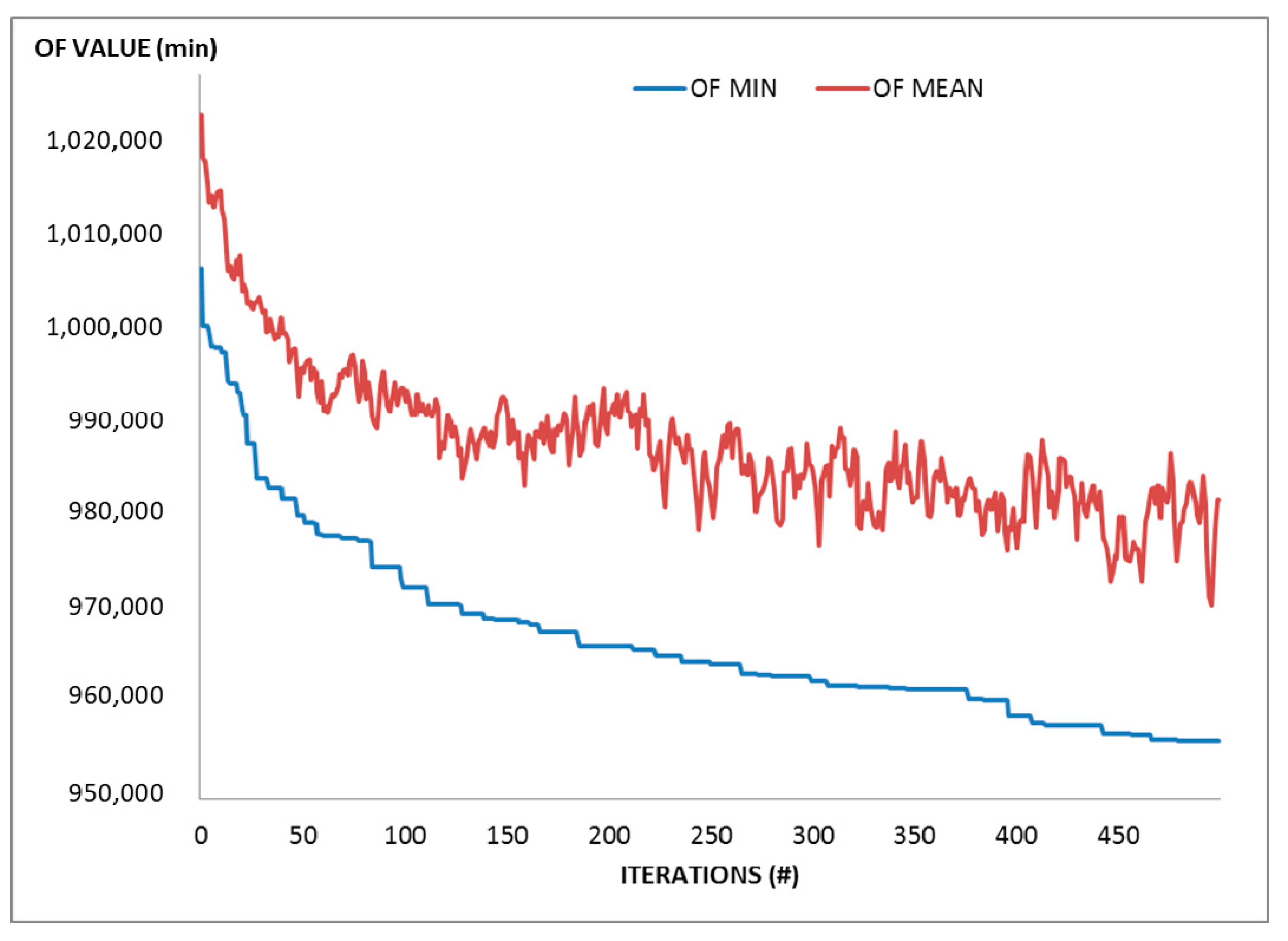For this scenario, a detailed comparison between the two algorithms is reported in the figures below: Figure 1 and Figure 2 show the trend of the OF minimum and mean value for the PSO and GA, respectively. The trend obtained by PSO algorithm is characterized by sudden increases of the mean value due to the speed updating procedure that adds random properties to the optimization method to investigate new valleys of the searching space without being trapped in local minima. Such high peaks are missing in the OF trend of the GA (Figure 2), underlining a smoother contribution of the random component to the search process.

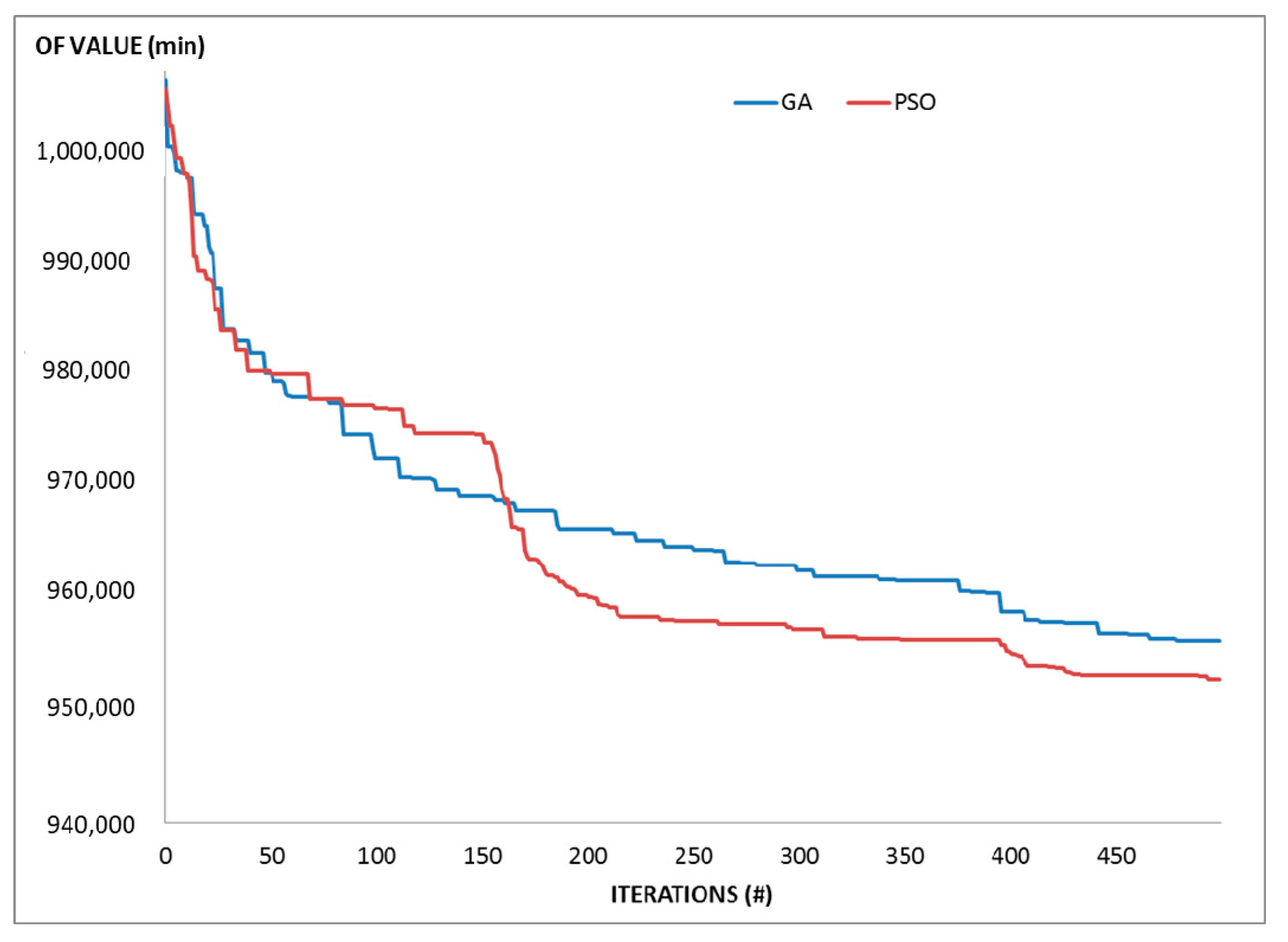
Figure 3 shows a straight comparison between trends of the GA and PSO OF minimum values. It allows to appreciate how PSO is more efficient than GA. The trend clearly shows that, after about the 150th iteration, the minimum OF value found by the PSO is lower than that of the GA. Moreover, this value is very close to the one reached by the GA in its last 100 iterations (from iteration #400 on). The results of the remaining scenarios confirmed the efficiency properties of the PSO algorithm.

The analysis of the transport effectiveness of the results obtained by the two optimization procedures is reported in

Table 2. OF terms for the different design networks (PSO and GA application).

Scenario	Algorithm	OF min	Veh.∙km	Uns. Demand (pax)	Boardings (pax)	Access Time (h)	Waiting. Time (h)	In-veh. Time (h)
EXISTING NETWORK (214 LINES)		1,102,602	18,912	14,206	320,817	101,656	33,131	99,906
40 LINES	PSO	989,290	11,094	6,982	323,477	104,809	22,583	80,493
	GA	984,260	11,583	6,958	322,612	103,419	22,765	81,681
55 LINES	PSO	963,467	12,745	5,896	320,388	100,296	22,406	82,100
	GA	977,757	12,347	6,878	328,919	101,236	22,822	82,215
85 LINES	PSO	956,967	15,174	5,311	324,706	97,522	22,014	82,361
	GA	965,661	14,997	5,651	325,823	97,336	22,155	83,031
110 LINES	PSO	956,751	15,671	5,354	334,851	95,802	22,725	83,299
	GA	961,299	16,583	5,634	333,625	95,734	22,301	83,962
130 LINES	PSO	952,837	16,994	5,121	330,065	95,099	22,083	83,497
	GA	956,228	16,816	5,044	329,120	95,774	22,293	82,858

and

Table 3. Comparison among OF parameters for different design networks with respect to the existing one.

Scenario	Algorithm	OF min	Veh.∙km	Uns. Demand (pax)	Boardings (pax)	Access Time (h)	Waiting. Time (h)	In-veh. Time (h)
EXISTING NETWORK (214 LINES)		-	-	-	-	-	-	-
40 LINES	PSO	−10.3%	−41.3%	−50.9%	0.8%	3.1%	−31.8%	−19.4%
	GA	−10.7%	−38.8%	−51.0%	0.6%	1.7%	−31.3%	−18.2%
55 LINES	PSO	−12.6%	−32.6%	−58.5%	−0.1%	−1.3%	−32.4%	−17.8%
	GA	−11.3%	−34.7%	−51.6%	2.5%	−0.4%	−31.1%	−17.7%
85 LINES	PSO	−13.2%	−19.8%	−62.6%	1.2%	−4.1%	−33.6%	−17.6%
	GA	−12.4%	−20.7%	−60.2%	1.6%	−4.2%	−33.1%	−16.9%
110 LINES	PSO	−13.2%	−17.1%	−62.3%	4.4%	−5.8%	−31.4%	−16.6%
	GA	−12.8%	−12.3%	−60.3%	4.0%	−5.8%	−32.7%	−16.0%
130 LINES	PSO	−13.6%	−10.1%	−63.9%	2.9%	−6.5%	−33.3%	−16.4%
	GA	−13.3%	−11.1%	−64.5%	2.6%	−5.8%	−32.7%	−17.1%

for any term of the objective function. The results are compared with current transit network (absolute values and percentages).

As shown in Table 3, among all the scenarios the OF terms vary in a limited range, except for the operator costs (vehicle∙kilometres) and the unsatisfied demand. In fact, the first term decreases with the reduction of the number of lines composing the network: the difference between the 40-bus-lines network and the 130-bus-lines network amounts to about −30%. The unsatisfied demand increases with the reduction of the number of lines composing the network: the difference between the 40-bus-lines network and the 130-bus-lines network amounts to about +15%. This is due to the large size of the entire network and reflects the need for a high number of lines to serve all 230,000 trips composing the potential transit demand in the morning peak hour. The remaining terms of the objective function indicate that design networks with few lines highly rely on a rapid rail system.

The comparison between the existing network and the best design network (130 lines networks) shows that Rome’s transit demand can be served effectively (reduction of 30% of the waiting time) by a bus network composed of a lower number of lines (reduction of almost 40%) in a more efficient way (reduction of 10% of the operating costs), still guaranteeing the same service area coverage as the current system.

It is important to underline that the designed network provides significant improvements in terms of in-vehicle time (reduction equal to about 16%) due to the increase of direct lines. A small increase is recorded for the number of transfers.

5. Conclusions

This paper proposes a PSO approach procedure for solving the bus network design problem. The solving procedure consists of a set of heuristics, which includes a first routine for route generation based on the flow concentration process, and a PSO algorithm to find an optimal or near-optimal network of routes with the associated frequencies. The main novelty introduced is the use of this optimal solution calculation technique and its application to a transit network design methodology. It was developed for a large urban area (the city of Rome), characterized by three aspects: (a) a complex road network topology, not simply represented as radial or grid network; (b) a multimodal public transport system (a rapid rail transit system, buses, and tramways lines); and (c) a many-to-many transit demand.

The robustness and effectiveness of the model in producing optimal solutions was proved and the PSO approach was demonstrated as suitable if combined with the HRGA. The application of the PSO algorithm to the set of routes created in the route generation step, from which the solving procedure created the swarm and particles for the optimal solution, highlighted that PSO is more efficient and effective than GAs. The analysis of the optimal solutions showed that PSO provides a lower minimum value of OF than the GA in most of the five created scenarios. These minimum values were also reached in a lower number of iterations. The best solution among the five provided scenarios (composed of 130 lines) shows the expected results also in the comparison between the OF components. In fact, transit demand can be served effectively (a reduction of 33% in waiting time) by a bus network composed of a lower number of lines (a reduction of 40%) in a more efficient way (a reduction of 10% in the operating costs), still guaranteeing the same area coverage as the current system.

Further developments might focus on a multi-objective approach in the definition of the OF terms and on the use of different optimization techniques, such as ACO algorithms. It would be worth testing this solving technique to feeder bus network design problems. The research agenda also includes an application of this procedure to a different version of Rome’s current network, with almost 1330 traffic zones. Finally, additional refinements and improvements of the PSO structure and parameters could be necessary for a further decrease in computational times.