Using Smart City Tools to Evaluate the Effectiveness of a Low Emissions Zone in Spain: Madrid Central

Abstract

Population concentration in cities brings new risks as an increase in pollution, which causes urban health problems. In order to address this problem, traffic reduction measures are being implemented as pedestrianization areas; they are the definition of Low Emissions Zones (LEZs). When the effectiveness of these types of measures is in doubt, smart city tools provide data that can be used to scientifically asses their impact. This article analyzes the situation of Madrid Central (Spain), a LEZ subject to controversy. We apply statistical and regression analyses to evaluate the effectiveness of this measure to reduce air pollution and outdoor noise. According to the results, this LEZ was able to significantly reduce NO${}_2$, PM${}_{2.5}$, and PM${}_{10}$ concentration locally, having the same positive impact in the rest of the city. In terms of noise, this measure was able to mitigate background noise levels generated by road traffic.

1. Introduction

Urbanization trends worldwide show a clear preference of the population to live in urban areas: Today, 55% of the world’s population lives in urban places and this proportion is expected to increase to 68% by 2050 [1]. The attraction of the city lies in the numerous opportunities resulting from the agglomeration of human capital and the associated economic dynamism. However, while it is true that urban areas are key for social change, wealth generation, and innovation, the concentration of people in cities also leads to new risks from an economic, social, and environmental point of view.

It is not uncommon for cities to be car-use oriented, with a design characterized by lack of safe public spaces that tend to discourage physical activity [2]. Nonetheless, the major concern derived from the rapid development of car-oriented cities is the high generation of emissions (air pollutants and noise) and their impact on the inhabitants’ health [3]. Another related problem is the increase of environmental noise, which gives rise to a range of health problems including annoyance, sleep disturbance, increasing hypertension, and cardiovascular diseases [4]. In this regard, the speed of urbanization has outpaced the ability of governments to build essential infrastructures that make life in cities safe, rewarding, and healthy [5].

As about 80% of this pollution associated with health problems is produced by cars [6], reducing traffic seems to be an efficient strategy to improve urban livability and inhabitants’ health. Thus, many cities around the world have started to shift toward non-car friendly access (pedestrianization measures) because it is an effective and non-expensive way to reduce air pollution and noise [3,7,8,9,10].

According to the European Commission, a smart city goes beyond the use of information and communication technologies (ICT) for better resource use and less emissions [11]. In fact, different smart city tools and smart city management can be invaluable for fulfilling the government’s commitment to the citizen. Taking advantage of this approach and, in order to measure effectiveness or even to scientifically guide the process, we can benefit from putting into use air quality monitoring and other tools that a smart city provides, e.g., internet of things (IoT) and open data.

In this work we analyze with smart city tools the effectiveness of the implementation of Madrid Central (MC), a Low Emissions Zone (LEZ) in Madrid, Spain. This approach is specifically needed there because of the controversy around MC and its use as a political symbol. Despite the fact that this LEZ was actually an extension and continuation of previous measures with the goal to comply with a European air quality requirement, MC encountered strong opposition. Those claiming the supposed right to go by car claimed this measure is ineffective concerning the reduction of pollutants and claim it is a cause of border effect (pollution displacement). Fulfilling its electoral promise, after the elections the new government decided to reverse the MC measures.

This article is an extension of a preliminary study in which this pedestrianization measure was locally evaluated in terms of its impact on the LEZ on a subset of pollutants [12]. The data used in that study comprises a time frame of 30 months (between December 2016 and May 2019), even if MC was active just during six months. According to the results obtained, the research concluded that MC was effective in reducing the concentration of NO${}_2$ and noise in the area.

This new analysis considers a longer amount of time and a more comprehensive range of pollutants. This piece also takes into consideration a bigger area of the city in order to check potential side effects. Therefore, in this article, we face the following research questions: RQ1: Is the deployment of MC effective at reducing the concentration of NO${}_2$ and so improving the air quality in this area? RQ2: Is the implementation of an LEZ an effective measure to reduce environmental noise levels?. RQ3: Do pedestrianization policies in a given area of the city produce a pollution displacement to other zones of the city?. RQ4: Are smart city tools effective for evaluating urban health policies and other measures implemented in the city?.

The main contributions of this study are: (i) It evaluates the effectiveness of traffic limitation measures in reducing emissions harmful to health; (ii) it analyzes the impact of such measures on environmental noise, which is also associated with poorer urban health; (iii) it checks whether the claim of pollution displacement (border effect) has any basis according to results; and (iv) it appraises the usefulness of smart city tools as an appliance for evaluating urban measures and policies to reduce pollution.

The paper is organized as follows: First, the impact of pollutants on health is reviewed, MC is contextualized, and related research is introduced. Section 3 introduces the materials and methods used in this analysis. Air quality and noise reduction are evaluated first locally (in the LEZ) and in the whole city in Section 4 and Section 5. Finally, Section 6 presents the conclusions and the main lines of future work.

2. Background

This section introduces first the main effects of car-use oriented cities on health. Next, it presents the EU directives on air pollution and the main aspects of the implementation of MC, including the municipal regulations on which it is based. Finally, it reviews relevant related work.

2.1. Are We Designing Cities for Cars or for People? The Effects on Health and Well-Being

The urban design of most cities prioritizes the use of motorized vehicles, thus relegating pedestrian travel. This approach to the city has a variety of negative impacts on safety and health, as well as on the general quality of life. An urban design focused on car use has a negative effect on the quality of the social space, forgetting that the physical and spatial context has a deep influence on people throughout the whole course of life. It has been proved how the growth of car use reduces children’s access to public space in urban contexts due to traffic and lack of infrastructure for pedestrians [13,14]. Restricting mobility is critical for the development of children’s spatial awareness and spatial activity, thus affecting their social and physical development [15]. Other groups, such as the elderly, could benefit too from environments with safe walking access, improving their independence and well-being [16].

Moreover, traffic and car use cause a high generation of emissions, both air pollutants and noise. This leads to a range of urban health problems: It reduces life expectancy, produces loss of years of a healthy life, and diminishes the quality of health [3]. Air pollution, which caused more than 400,000 premature deaths in 2016, is considered the top health hazard in the European Union (EU) [17,18]. It has proved to be associated with heart disease and strokes, lung diseases, and lung cancer, besides reducing lung capacity and aggravating asthma. Air pollution has been also pointed out as carcinogenic and causes infertility and diabetes type 2 [19]. Other studies link air pollution to obesity, systemic inflammation, ageing, Alzheimer’s disease, and dementia [20]. It also affects the brain in the same way that Alzheimer’s does as it causes changes in the structure of the brain [21]. While pollution affects all ages, some population groups are more vulnerable to pollution problems, such as pregnant women, newborns, children, and the elderly. It also can exacerbate preexisting conditions at all ages.

Environmental noise is the major preventable cause of hearing loss [4]. It can also cause a range of non-auditory problems. To begin with, the evidence for the effects of environmental noise on health is strongest for annoyance, sleep disturbance, and cognitive performance in both adults and children [22]. Sound pollution also affects the cardiovascular system and causes hypertension [4,22]. Among children, it generates cognition problems, such as communication difficulties, impaired attention, increased arousal, frustration, and worse performance [23,24]. Last but not least, noise pollution causes annually at least 16,600 cases of premature death in Europe [25].

These risks could be reduced by limiting car use. Among different approaches to reducing car use, pedestrianization and LEZ have been proved as some of the most effective strategies against emissions. Absolute pedestrianization is difficult to implement (and expensive) but LEZs have proved to be successful in different European Member States. These are the cases for the LEZ (“Umweltzone”) for trucks and cars in the center of Berlin inside the S-Bahn ring (Germany); the LEZ in the Lombardy Region for motorcycles, buses (whole year), and vehicles during wintertime, e.g., in Milan (Italy); or the LEZ for vans and lorries in Greater London (United Kingdom). All of these experiences have registered good results in terms of improving air quality.

2.2. Reducing Pollution: International Directives and the Low Emissions Zone in Madrid

While cities are related to social and economic progress, the increase of air pollution and noise can be considered a modern plague [26] decreasing the quality of life in cities [27]. In Europe (where 74% of the population lives in urban areas) the concern on this matter has led to the creation of a common set of environmental rules. These directives could not just safeguard EU citizens from environment-related pressures and risks to health and well being, but also reduce significantly different expenses: An adequate implementation of environmental legislation could save 50 billion euro every year in health and environment costs to the EU economy [20].

Because of this, a Clean Air Policy Package is adopted in 2013 by the the European Commission. This air quality policy, based on Directives 2008/50/EC [28] and 2004/107/EC [29] rests on three pillars: (i) Air quality standards; (ii) national emission reduction targets established in the National Emissions Ceiling Directive; and (iii) emissions standards for key sources of pollution (such as cars).

Noise being another harmful hazard, the EU regulation (Directive 2002/49/EC) [30], for every Member State: (i) Establishes the creation of noise mapping to determinate exposure levels to environmental noise; (ii) makes environmental noise information available to the citizens; (iii) establishes adoption of action plans, based upon noise-mapping results, to prevent and reduce environmental noise where necessary.

The referred to directive points out that road traffic is a majors source of noise; it has also been noted as the largest contributor to nitrogen oxide emissions [31]. For the reasons alluded to previously, NO${}_2$ is one of the main concerns of the EU: Exposure to air pollution from road transport costs about 137 billion per year in Europe [32] but, more important, it produced around 76,000 premature deaths in 2015 [33]. Despite this, a number of countries keep exceeding the maximum established PM${}_{10}$ and NO${}_2$ levels. Spain is one of them, with several urban areas under surveillance by the EU because of their poor air quality. The European Commission required the reduction of these air pollutants under the threat of penalties.

Madrid City Council decided to reduce transit traffic in a delimited area of the downtown, replicating other European experiences. Madrid Central is an LEZ in Madrid, consisting of a number of car access restrictions for non-residents, independent from the current pollution level of the air.

The clarity in the perimeter of MC is one of their virtues, so facilitating the understanding of zonal delimitation and helping to introduce a behavioral change in the city.

MC is created by the Ordenanza de Movilidad Sostenible (5 October 2018) and it covers almost the entire Centro district, which is formed by the neighborhoods of Palacio, Embajadores, Cortes, Justicia, Universidad, and Sol. In this area, of 4,720,000 m${}^2$, Centro contains 134,881 people, of which 21.6% are over 65 years old and 9.2% are less than 17 years old. Children and the the elderly are the age groups which can benefit more from the reduction of noise and pollutants.

The goal of MC is to improve air quality, but also to respond to the idea of changing the uses of spaces in the city center, prioritizing the pedestrian one and reducing noise pollution. However, as we said, its conformation mainly responds to ensuring the objectives demanded by the EU. The traffic restriction started on 30 November 2018, and the fines for noncompliance did not start until 16 March 2019. Thanks to this straightforward measure, Spain avoided being brought to the European Court of Justice and so, the economic fine.

However, the measure raised strong opposition from some political parties. After the elections (held on 26 May 2019) and qualifying the MC measures as inefficient and even unnecessary, the newly elected government approved article 247 of the Ordenanza de Movilidad Sostenible, applying with it a moratorium on fines from 1 July to 30 September 2019. Besides a warning from the EU, the decision raised social protests, especially from environmental groups. This suspension led to the emergence of social movements claiming the paralysis of this reversal based on the negative effects on health and environment, and a warning from the EU. Finally, after a contentious administrative appeal filed by the Platform in Defense of Central Madrid, a judge reactivated MC, suspending the moratorium on fines.

2.3. Related Works

The proliferation of pedestrianization measures and policies in different cities has led to a number of studies to evaluate their efficacy. A brief review of the related literature is presented next.

The impact of the rapid growth of car ownership in Beijing, China was analyzed in terms of transportation, energy efficiency, and environmental pollution [34,35] A set of measures were applied in Beijing in 2010 to mitigate the effects of traffic congestion and reduce air pollution. Liguang et al. [34] analyzed data from Beijing Municipal Committee of Transport to evaluate the implementation of car use restriction measures. Fairly good effects on improving urban transportation and air quality were achieved according to the results reported. Liu et al. [35] proposed an indirect approach to evaluate the impact of car restrictions and air quality, by applying a generalized additive model to explore the association of driving restrictions and daily hospital admissions for respiratory diseases. Several interesting facts were obtained from the analysis, including higher daily hospital admissions for respiratory disease for some days, and the stronger effect on cold season. Females and people older than 65 years benefited more from the applied environmental policy. Overall, the authors found positive effects on the improvement of public health. More research had been performed addressing the LEZ analysis in China [36,37,38].

In Europe, more than 200 LEZ have been deployed in recent years [39]. Studies on their impact on urban air quality have been performed in several countries: Netherlands [40,41], Denmark [42], United Kingdom [43,44], Germany [45,46], Italy [47], and Portugal [48,49]. Most of them analyzed and acknowledged the reduction of two hazardous pollutants: Nitrogen dioxide (NO${}_2$) and particulate matter (PM).

Regarding noise pollution, there is a body of work on analyzing urban noise and its impact on the population’s health [50,51,52,53,54,55]. There are only a few studies done in this regard [12,56]. However, most of the studies presented above studied also some variables related to noise pollution.

Focusing on Madrid, air quality has been a health issue over recent decades. Thus, there are several studies dealing with air pollution in this city. Borge et al. [57] reported the modeling activities carried out in Madrid, emphasizing the atmospheric emission inventory development, which comprises the combination of models and real data. They showed that Madrid required a reduction in NO${}_x$ emissions in order to meet the NO${}_2$ European standards, which was the main motivation behind the implementation of MC. Different models were used to simulate and evaluate a short-term action plan to mitigate pollution emissions [58,59]. More recently, after the application of MC, Lebrusán and Toutouh [12] evaluated the effectiveness of this measure in reducing pollution inside the LEZ. Another study applied computational intelligence (deep neural networks and regression analysis) to evaluate the evolution of NO${}_2$ concentration in the air, but again only locally (inside the MC area) [60]. Both reported a decrease in NO${}_2$ concentration. Our article contributes to this line of research by extending the set of pollutants studied by adding PM, among others, taking into account a longer time frame, and including 24 areas of study in order to get a more general idea of the impact of this type of measures in the whole of Madrid.

3. Materials and Methods

The primary goal of this study is to take advantage of smart city tools, such as a sensor network and open data, to evaluate the effects of an LEZ on environmental pollution and noise. We address such an analysis, first locally, evaluating the impact of this measure at the MC area, and globally, by assessing the same in different areas of the city (Madrid).

Madrid City Council installed different sensors (see Figure 1) that gather data on the ambient concentration of different pollutants and measure the output noise levels. The data is available on the Open Data Portal (ODP) Madrid City Council (URL: https://datos.madrid.es/). We use such open data in this research.

The analysis is performed considering a temporal frame of six years (72 months), from December 2013 to November 2019. Two periods are distinguished: Pre-MC, i.e., the period of five years before implementing MC (from December 2013 to November 2018), and Post-MC, i.e., the period of one year after implementing the mobility measure (from December 2018 to November 2019). The main idea is to compare both periods to asses the effect of the measures applied in MC.

In the following, we introduce the air pollutants analyzed, the outdoor noise metrics studied, and the methodology applied in the evaluation.

3.1. Air Quality Evaluation

The Open Data Portal (OPD) provides the hourly mean concentration of several air pollutants. In this study we focus on six: Sulfur dioxide (SO${}_2$), nitrogen dioxide (NO${}_2$), ozone (O${}_3$), carbon monoxide (CO), particulate matter 10 micrometers or less in diameter (PM${}_{10}$), and particulate matter 2.5 micrometers or less in diameter (PM${}_{2.5}$).

Table 1. Maximum concentration allowed of pollutants in the air by the WHO and EU regulations.

Pollutant	Averaging Period	WHO Theshold Concentration	EU Theshold Concentration
${\mathrm{SO}}_2$	24 h	20 $\mathsf{\mu }$g/m${}^3$	125 $\mathsf{\mu }$g/m${}^3$
	1 h	-	350 $\mathsf{\mu }$g/m${}^3$
	10 min	500 $\mathsf{\mu }$g/m${}^3$	-
${\mathrm{NO}}_2$	1 year	40 $\mathsf{\mu }$g/m${}^3$	40 $\mathsf{\mu }$g/m${}^3$
	1 h	200 $\mathsf{\mu }$g/m${}^3$	200 $\mathsf{\mu }$g/m${}^3$
${\mathrm{O}}_3$	8 h	100 $\mathsf{\mu }$g/m${}^3$	120 $\mathsf{\mu }$g/m${}^3$
$\mathrm{CO}$	8 h	10 mg/m${}^3$	10 mg/m${}^3$
${\mathrm{PM}}_{10}$	24 h	50 $\mathsf{\mu }$g/m${}^3$	50 $\mathsf{\mu }$g/m${}^3$
	1 year	20 $\mathsf{\mu }$g/m${}^3$	40 $\mathsf{\mu }$g/m${}^3$
${\mathrm{PM}}_{2.5}$	24 h	25 $\mathsf{\mu }$g/m${}^3$	25 $\mathsf{\mu }$g/m${}^3$
	1 year	10 $\mathsf{\mu }$g/m${}^3$	-

summarizes the maximum concentration allowed in the studied pollutants established by WHO and EU directives.

3.2. Noise Evaluation

It is not trivial to chose the right parameters to evaluate noise pollution and its impact on the people. The sound-meters return measures that describe the physical attributes of the sound, but not the subjective response and the extent of the physiological and psycho-social harm done to the public. The noise pollution data provided by the OPD include the daily mean of the equivalent sound pressure levels, the percentile noise levels [61], and the noise pollution level (NPL) [62]:

• Equivalent sound pressure levels (L${}_{eq}$) can be described as the average sound level for the measurement. The data analyzed include the L${}_{eq24}$ that corresponds to the noise measured during the whole day (24 h). In addition, three L${}_{eq}$ are returned by taking into account the period of the day: L${}_{eqD}$, L${}_{eqE}$, and L${}_{eqN}$, which are evaluated during the day (from 7:00 h to 19:00 h), evening (from 19:00 h to 23:00 h), and night (from 23:00 h to 7:00 h), respectively.
• Percentile noise levels (L${}_x$) are the levels exceeded for x percent of the time, where x is between 0.1% and 99.9%. L${}_x$ is calculated by applying statistical analysis. We evaluate the L${}_{10}$, L${}_{50}$, and L${}_{90}$. The L${}_{10}$ and L${}_{90}$ are extensively used for rating any annoying traffic noise and background noise, respectively.
• NPL was developed to estimate the dissatisfaction caused by road traffic noise comprising the continuous noise level (L${}_{eq}$) and the annoyance caused by fluctuations in that level. NPL is equal to L${}_{eq}$ plus 2.56 times the standard deviation of the noise distribution and it is generally approximated by Equation (1).

$$NPL\approx L_{eq}+(L_{10}-L_{90})$$

(1)

All sound levels referred to in this article are measured in terms of an A-weighted decibel (dBA), which corresponds to the A-weighted sound level readings to replicate the response of the human ear to the annoyance caused by road traffic noise.

The Guideline Development Group (GDG) of WHO strongly recommends reducing L${}_{eq}$ noise levels produced by road traffic below 53 dBA. Road traffic noise above this level is associated with adverse health effects. Specifically, for night noise exposure (L${}_{eqN}$), the GDG strongly recommends reducing noise levels produced by traffic flows below 45 dBA, since road traffic noise above this level is associated with adverse effects on sleep [63]. According to the Community of Madrid regulations presented in the Normativa de ruido diurno y vibraciones [64], the L${}_{eq}$ levels should be between 50 and 65 dBA during the daytime and between 40 and 55 dBA during the night.

3.3. Methodology

In order to asses the effectiveness of the LEZ (see Section 2.2), we evaluate the air pollution and the noise in the LEZ and in different areas of the city. Thus, we asses the local effect on the LEZ area and whether it is possible that a border effect is occurring as a result of potential traffic diversion (i.e., check the existence or absence of the border effect). The analysis performed in this article mainly considers:

• The pollutant concentration or level of noise itself during both periods Pre-MC and Post-MC, which is measured and averaged for periods of one hour and one day.
• The average difference between the pollutant concentration or level of noise x during Post-MC ($x_{Post-MC}^m$) and Pre-MC ($x_{Pre-MC}^m$), taking into account different months (M). We denote this metric by $\Delta$ (see Equation (2)). Negative values of $\Delta$ denote reduction/improvement of x.
• The percentage of the time the population is exposed to air pollutant concentration or noise levels below the thresholds defined by EU denoted by $\tau$. These thresholds are shown in Table 1. The value of $\tau$ allows the assessment of the effectiveness of MC to potentially improve urban health because there may be situations where the pollution or noise is reduced but the situation is still unhealthy according to the EU regulations (e.g., NO${}_2$ concentration > 40 $\mathsf{\mu }$g/m${}^3$).
• Polynomial regression is applied to evaluate the general trend in air pollution concentration or levels of noise with and without the implementation of the road traffic restrictions in Madrid Central. While it is one of the simplest methods for analysis and estimation of time series, it is frequently used in the related literature [12,35,38] In this article, two polynomial regression methods are studied: Linear and polynomial of grade 10.

$$\Delta =\frac{1}{\left|M\right|}\sum _{m\in M}{x}_{Pre-MC}^m-x_{Pre-MC}^m$$

(2)

In order to determine the statistical significance of the results obtained, Shapiro–Wilks statistical test is applied to check the normality of the distributions and, as the results are not normally distributed, Mann–Whitney U rank test is used to asses if the pollutant is statistically reduced during Post-MC.

4. Pollution Evaluation at the LEZ Area

This section analyzes the information gathered by the sensor located in Pza. del Carmen (id. 35), which is the one inside the LEZ. When evaluating the pollution in MC, we face two main drawbacks: fFrst, the sensor does not gather information about PM${}_{2.5}$ and PM${}_{10}$, and second the noise data shared through ODP does not provide complete data for 2013. Thus, we do not include in this section the analysis of these two air pollutants and the Pre-MC period is defined from December 2014 to November 2018 when the noise is evaluated.

4.1. Air Quality

Table 2. Summary of the air pollutants sensed. Negative values of $\Delta$ indicate a reduction of pollution and check-mark (✓) illustrates that there is statistical difference (p-value < 0.01).

Season		Pre-MC					Post-MC					$\Delta$
		Min	Median	Iqr	Max		Min	Median	Iqr	Max
SO${}_2$ concentration in $\mathsf{\mu }$g/m${}^3$
spring		1.00	7.33	4.39	37.00		6.76	12.11	1.42	24.00		39.45
summer		1.00	8.90	5.94	50.00		1.00	10.49	1.98	17.00		15.19
autumn		1.00	8.33	5.53	53.00		1.00	11.69	6.38	35.00		28.70
winter		1.00	7.92	5.08	53.00		6.34	15.25	4.70	68.00		48.06
NO${}_2$ concentration in $\mathsf{\mu }$g/m${}^3$
spring		5.00	38.39	20.30	162.00		1.00	23.92	16.39	131.00		✓ −60.47
summer		3.00	39.79	22.74	196.00		8.00	34.33	19.46	139.00		✓ −15.88
autumn		1.00	56.37	26.31	224.00		5.00	41.68	23.93	123.00		✓ −35.25
winter		4.00	51.05	25.43	196.00		1.00	49.63	26.00	147.00		−2.86
O${}_3$ concentration in $\mathsf{\mu }$g/m${}^3$
spring		1.00	55.05	27.35	157.00		4.00	59.94	21.91	131.00		8.16
summer		1.00	63.40	32.83	215.00		1.00	52.74	26.45	135.00		✓ −20.20
autumn		1.00	26.49	22.80	134.00		1.00	31.77	21.26	112.00		16.61
winter		1.00	26.99	19.97	102.00		2.00	31.47	24.06	98.00		14.24
CO concentration in mg/m${}^3$
spring		0.10	0.31	0.13	1.90		0.10	0.54	0.24	3.00		43.06
summer		0.10	0.33	0.21	2.30		0.10	0.27	0.28	3.00		✓ −21.38
autumn		0.10	0.47	0.30	2.60		0.10	0.50	0.26	2.00		5.31
winter		0.10	0.45	0.27	2.90		0.10	0.45	0.34	4.10		✓ 0.17

reports the minimum (Min), the maximum (Max), the median (median), and the interquartile range (Iqr) for the concentration of the pollutants sensed in MC during the two periods analyzed here. The last column includes the value of $\Delta$, and the check-mark (✓) indicates that there is a statistical difference according to the Mann–Whitney U test in such a pollutant for the periods analyzed (i.e., p-value < 0.01).

Table 3. Percentage of time $\tau$ the air pollutant concentration is lower than the EU thresholds.

Period	SO${}_2$	NO${}_2$	O${}_3$	CO
Pre-MC	95.81	46.88	97.96	100.00
Post-MC	94.48	62.17	99.63	100.00

presents the percentage of time $\tau$ that the air pollutant concentration is lower than the threshold defined by the EU.

The evaluated measures are grouped by season because the meteorological conditions (i.e., wind direction and speed, atmospheric pressure, temperature, and relative humidity) affect the chemical behavior of the evaluated pollutants [65].

Figure 2 and Figure 3 show the mean concentration of SO${}_2$ and NO${}_2$ by month, respectively. Notice that Pre-MC covers a longer amount of time. These figures also illustrate the boxplot of the concentration of the air pollutants for Pre-MC and Post-MC periods and the probability density function (PDF) of the whole data grouped by periods, i.e., Pre-MC and Post-MC. Figure 4 illustrates the regression analysis to evaluate the general trend of NO${}_2$ through the time. Finally, Figure 5 and Figure 6 show also the mean concentration of O${}_3$ and CO by month, respectively.

The concentration of ${\mathrm{SO}}_2$ in the air is higher during Post-MC than during Pre-MC for all seasons (i.e., $\Delta >0$). Figure 2 illustrates this increase. This is principally due to the largest sources of SO${}_2$ emissions being fossil fuel combustion at power plants and other industrial facilities [65]. Thus, mobility-related measures or policies are not appropriate for reducing SO${}_2$ concentration in the air.

For both periods, the mean concentration does not exceed the threshold defined by the EU (20 $\mathsf{\mu }$g/m${}^3$); however, the maxima values do (see Table 2). Table 3 shows that the population is under an SO${}_2$ concentration lower than the UE threshold during 95.81% of the time for Pre-MC and 94.48% for Post-MC. Thus, the excess of this pollutant is exceptional and negligible, so it is not considered problematic in Spain.

Focusing on NO${}_2$, which is the pollutant that almost led Spain to the European Court and the excess of which is a public health concern, its concentration is significantly reduced for all seasons, except winter (i.e., Mann–Whitney U statistical test p-value < 0.01). The decrease of NO${}_2$ concentration is lower during winter because of the heavier use of combustion power plants for wintertime home heating (therefore, road traffic may not be the main source of NO${}_2$), and also because of the fact that NO${}_2$ stays in the air longer in the winter [65]. Figure 3b confirms that warmer seasons have better air quality.

As can be seen in Figure 3a, the concentration of NO${}_2$ exceeds, during several months, the maximum one allowed by the EU for both periods (Pre-MC and Post-MC) but with important differences. Thus, Table 3 results indicate that the population had healthier air for 15.29% longer duration during Post-MC as compared to Pre-MC circumstances (62.17%-46.88%). Figure 3c confirms that MC is under lower concentration of NO${}_2$ in the air during Post-MC.

It is noticeable that there is a clear downward trend in the concentration of NO${}_2$ after the application of the car restrictions (see Figure 3a). We apply regression analysis to evaluate the general trend of this pollutant. Figure 4 illustrates two different experiments: First, we take into account all the hourly concentration values during the last two years to see the trend of the closest time (a), and second the sensed values are averaged by month and the trends for the five years previous to the MC measurements (from 2014 to 2018) and also for the last five years (from 2015 to 2019) are evaluated (b). This last experiment analyzes the possible change of trend due to the new mobility policies.

In Figure 4a, the polynomial regression of grade 10 (black line) shows, first, how NO${}_2$ concentration increases during colder seasons and decreases in warmer ones and, second, that the pollution values during Post-MC are lower than Pre-MC. In turn, the linear regression (black dashed line) displays a declined trend over time for this air pollutant. In Figure 4b, the black dashed line that represents the linear regression of NO${}_2$ concentration before applying MC (five years) has a positive slope (i.e., the NO${}_2$ concentration tends to increase). The solid black line that represents the general trend after applying MC measures has a negative slope, which indicates that NO${}_2$ concentration in the air tends to be reduced. Thus, the behavior of the concentration of NO${}_2$ in the air under the application of MC measures points out that the traffic restriction has a positive effect on air quality.

The concentration of O${}_3$ shows a similar behavior for both periods (see Figure 5 and Table 3). The results in Table 2 show that the concentration of this pollutant increased after the application of MC during spring, autumn, and winter, but it decreased during summer. All the monthly average O${}_3$ values are lower than the maximum defined by the EU (120 $\mathsf{\mu }$g/m${}^3$). According to Table 3 values, the population is almost all the time experiencing air without an excess of O${}_3$ during Post-MC.

The increment of O${}_3$ that we illustrate in our analysis could be due to the oxidation of NO, i.e., the chemical reaction of O${}_3$ and NO that forms NO${}_2$ and O${}_2$, which occurs in urban areas [66]. As the road traffic limitation reduces the concentration of NO, the portion of O${}_3$ that reacts with NO is lower. Therefore, the levels of O${}_3$ do not decrease, and subsequently the concentration of NO${}_2$ produced by the oxidation of NO is lower. In short, this upturn can be a chemical consequence of the reduction in the air of other components’ concentrations.

Regarding CO, as it occurs with O${}_3$, the concentration of this pollutant decreases during summer, but increases during the other seasons (see Table 2 and Figure 6). While one of the major sources of this pollutant concerning outdoor air is road traffic vehicles or machinery that burn fossil fuels, it seems that the reduction of road traffic does not lead to a decrease of CO in this case. However, according to EU regulations, there is not a need to reduce CO since during the time frame analyzed in this article there is not any measurement over the threshold stipulated by the EU (10 mg/m${}^3$).

Finally, the evaluation of SO${}_2$, NO${}_2$, O${}_3$, and CO indicates that the final environmental balance may not always coincide with what was intuitively expected. However, it is important to remark that MC measures are highly effective in reducing NO${}_2$ concentration, which was one of the major motivations for making this move. Therefore the answer to RQ1 (is the deployment of MC effective at reducing the concentration of NO${}_2$ and so improving the air quality in this area?) is yes. The restriction to the road traffic applied in MC has significantly reduced NO${}_2$ concentration.

4.2. Outdoor Noise in MC Area

Table 4. Summary of the levels of noise (in dBA). Negative values of $\Delta$ indicate a reduction of pollution and check-mark (✓) illustrates that there is statistical difference between the periods analyzed (p-value <  0.01).

Season		Pre-MC					Post-MC					$\Delta$
		Min	Median	Iqr	Max		Min	Median	Iqr	Max
L${}_{eq24}$		59.30	67.50	1.70	95.80		62.30	66.70	1.62	77.30		✓ −0.34
L${}_{eqD}$		58.80	68.20	2.20	84.00		60.70	67.50	2.22	80.10		✓ −0.22
L${}_{eqE}$		57.10	67.80	1.67	82.00		57.80	67.20	1.50	82.60		✓ −0.46
L${}_{eqN}$		55.10	64.90	2.50	80.70		58.50	64.40	2.33	78.40		✓ −0.55
L${}_{10}$		62.70	70.70	1.70	81.50		66.40	70.00	1.60	86.70		✓ −0.37
L${}_{50}$		55.00	65.30	2.00	71.60		57.50	64.40	2.10	71.50		✓ −0.71
L${}_{90}$		47.30	56.90	2.50	66.30		49.80	56.20	2.50	63.40		✓ −0.77
$NPL$		68.70	80.90	3.00	108.40		74.90	80.10	2.80	100.50		✓ −0.00

reports the minimum (Min), the maximum (Max), the median (median), and the interquartile range (Iqr) of the levels of noise sensed in MC during the two periods analyzed here. The last column includes the value of $\Delta$ and the check-mark (✓) indicates that there is a statistical reduction in such a noise level between Pre-MC and Post-MC according to the Mann–Whitney U test (i.e., p-value < 0.01).

Table 5. Percentage of time $\tau$ the levels of noise are lower than the EU thresholds.

Period	L${}_{\mathit{eqE}}$	L${}_{\mathit{eqD}}$	L${}_{\mathit{eqN}}$
Pre-MC	4.94 (3.04)	8.30 (3.47)	0.00 (9.93)
Post-MC	3.02 (2.39)	9.89 (3.22)	0.00 (9.38)

presents the percentage of time $\tau$ that the outdoor noise levels are lower than the threshold values defined by Madrid City Council [64] (see Section 3.2). Figure 7 and Figure 8, and show the mean of the noise level evaluated here grouped by month.

Regarding the equivalent sound pressure levels (L${}_{eq24}$, L${}_{eqD}$, L${}_{eqE}$, and L${}_{eqN}$), the level the noise is higher during the hours between 7:00 h and 23:00 h than during the night time (see Table 4 and Figure 9). This is mainly due to the MC neighborhood being located in a commercial area and the business hours in Madrid usually ending at 22:00 h; thus, there is road traffic until late hours. There is a reduction in the median of all these noise levels during Post-MC. Therefore, in general, the noise is lower during this period. The highest differences between the two evaluated periods are given by the evening (L${}_{eqE}$) and night (L${}_{eqN}$) noise levels (see Table 4).

Focusing on Post-MC time, the levels of noise decrease during the first months but they experience an increase after June, i.e., when MC suffered from the reversal (see Figure 7). If we focus on L${}_{eq24}$ and L${}_{eqD}$, this increment is important. Taking into account the noise levels before the reversal, the reduction $\Delta$ for these two levels of noise is significantly higher, i.e., $\Delta \left(L_{eq24}\right)$ = −0.52 dBA and $\Delta \left(L_{eqD}\right)$ = −0.45 dBA. Thus, we can observe a negative impact on the noise pollution of the reversal that is mainly experienced at the time between 7:00h and 19:00h.

Evaluating $\tau$ during Pre-MC and Post-MC, Table 5 shows that the outdoor levels of noise practically always surpass the thresholds of the city council. During the night the levels of noise are never lower than 55 dBA, which is the threshold for these hours. Notice that we are evaluating equivalent sound pressure levels averaged for every day. Figure 7 also illustrates how the noise levels generally exceed the thresholds, i.e., the monthly average levels of noise are higher than 65 dBA for L${}_{eqD}$ and L${}_{eqE}$ and higher than 55 dBA for L${}_{eqN}$. Therefore, other measures must be applied to further reduce outdoor noise in this area.

Focusing on the percentile noise levels (L${}_{10}$, L${}_{50}$, and L${}_{90}$), Pre-MC and Post-MC differences are statistically significant. The best improvement $\Delta$ is shown by L${}_{90}$ (see Table 4), which represents the residual background levels of noise of the urban area analyzed. As the continuous road traffic flow is one of the main sources of the background noise, the reduction of traffic transit provokes a decrease in this type of noise.

L${}_{50}$, which statistically represents the median of the fluctuating levels of noise, is also reduced, i.e., $\Delta \left(L_{50}\right)$ = −0.71. The reduction of the annoying peaks in noise (i.e., L${}_{10}$) is lower than for the other two percentile levels ($\Delta \left(L_{10}\right)$ = −0.37). This represents a limited decrease of 0.5% regarding the median value of this noise during Pre-MC (70.70 dBA).

There is not a statistically significant reduction of NPL (see Table 4) and the average improvement is 0.00. Besides, as the computation of this metric depends on L${}_{eq24}$, it undergoes the same increase during the last months of Post-MC after the reversal of MC (see Figure 10).

Figure 11, Figure 12 and Figure 13 illustrate the trend of some representative levels of sound (L${}_{eq24}$, L${}_{eqD}$, and L${}_{90}$). When evaluating the trend of the last two years (on top of each figure), we observe similar behavior: (a) The polynomial regression of grade 10 (black line) illustrates the most marked reduction of the levels of noise during Post-MC until June 2019 when the MC was reversed, and (b) the linear regression (black dashed line) shows that the noise in MC is marginally reduced over time (i.e., the function presents negative slopes but close to zero).

At the bottom of Figure 11, Figure 12 and Figure 13, the black dashed lines that represents the linear regression of the levels of noise before applying MC (from 2014 to 2018) have slopes close to zero or even positive in the case of L${}_{eqD}$, i.e., there is an increase of outdoor noise in the area. The solid black line that represents the general trend after applying MC measures (last four years) has a steeper negative slope, which is higher in the case of L${}_{90}$. Thus, the car restrictions tend to improve the background noise generated by road traffic.

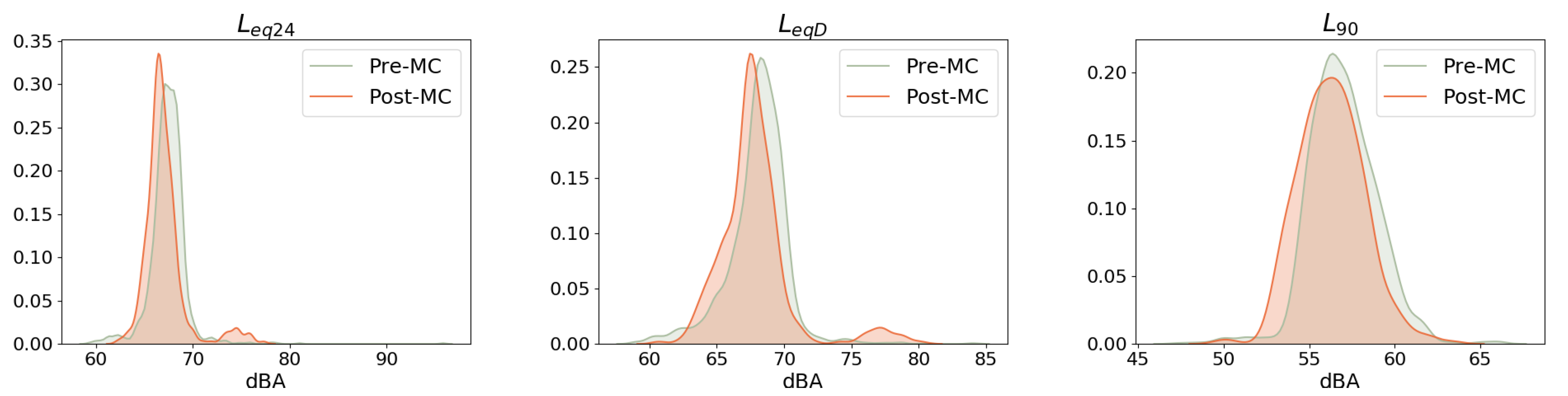
Finally, we have computed the PDF of the L${}_{eq24}$, L${}_{eqD}$, and L${}_{90}$ noise values to confirm that there is a slight reduction in the outdoor levels of noise in the area of MC. Figure 14 illustrates that the distributions of values detected Post-MC are more likely to be lower than the Pre-MC ones (the Post-MC distribution is lightly shifted to the left). However, while there is such a reduction, it is notorious that other types of measures are needed to mitigate this source of health problems and discomfort because the levels of noise exceed the thresholds set by the institutions nearly all the time during both evaluated periods, Pre-MC and Post-MC.

According to these results, we answer RQ2: Is the definition of an LEZ an effective measure to reduce environmental noise levels?. MC slightly reduces the outdoor levels of noise, mainly the background noise produced by road traffic. However, this decrease is not enough to keep the noise in the range of healthy levels.

5. Indirect Repercussion on the Pollution of the Whole City

According to the WHO and the EU, NO${}_2$ and particulate matter (PM${}_{2.5}$ and PM${}_{10}$) are the main culprits in public health problems due to pollution. This section aims at taking advantage of the sensors network installed in Madrid to:

• First, confirm that the important reduction of NO${}_2$ emissions in the MC area does not lead to an increase of that pollutant in other zones due to a hypothetical redirection of traffic to other areas of the city, i.e., to investigate the possible border effect of MC, and
• second, analyze the concentration of the particulate matter in the areas where the sensors gather such information in order to asses the possible impact on this aspect of the city due to MC measures.

The data provided by the ODP is incomplete and contains errors for several of the areas covered by the sensors. Only the data coming from sensors that correctly registered values for the whole time frame analyzed here are used in this analysis. Therefore, this section discusses data about NO${}_2$ from 23 sensors, PM${}_{2.5}$ from six, and PM${}_{10}$ from 12. This limits the areas of Madrid analyzed in our article. However, it ensures that the data reflect reliably the concentration in the air of the pollutants analyzed.

5.1. Temporal Variation in the Air Pollutants

In order to better understand the impact of NO${}_2$, PM${}_{2.5}$, and PM${}_{10}$ in Madrid, we evaluate their monthly trends that are shown in Figure 15. As seen in Section 4.1, NO${}_2$ exhibits seasonal variations, with the highest concentrations in winter and the lowest in summer. During warmer months (from March to September) the median NO${}_2$ concentration is lower than the EU threshold (40 $\mathsf{\mu }$g/m${}^3$). The highest NO${}_2$ concentration occurs during December and the lowest one during August.

This seasonal variation is mainly due to two different factors: The meteorological conditions and the emissions patterns. For example, temperature inversions and lower boundary layer heights in winter can cause NO${}_2$ not to be ventilated from the boundary layer, leading to higher concentrations in European cities. In contrast, the increase of photochemical activity, solar radiation, etc., during summer lowers NO${}_2$ concentration [67]. In addition, fossil fuel combustion sources such as residential coal and biomass combustion for heating also contributed to the formation of high NO${}_2$ concentration in wintertime.

Focusing on PM${}_{2.5}$, the highest concentration of this pollutant occurs in December (as with NO${}_2$). This pollutant presents a decreasing trend from December to May, springtime being the least polluted season. March, April, and May median values are the only ones that are lower than the threshold marked by the EU. For the months between June and November, the PM${}_{2.5}$ concentrations tend to be slightly higher than the EU threshold and similar to each other. PM${}_{10}$ shows a similar seasonal variation to PM${}_{2.5}$; from December to May there is a decrease in the concentration of this pollutant. July is the month with the highest PM${}_{10}$ concentration and May the month with the lowest one. In the case of this pollutant, June, July, August, and October median values surpass the EU threshold (40 $\mathsf{\mu }$g/m${}^3$).

5.2. Effect of Mobility Restrictions on NO${}_2$ Concentration in Other Areas of the City

The application of restrictions to vehicles in accessing a street or area affects the mobility patterns of the inhabitants in the whole city [3], and therefore impacts on the pollution in different areas of that city. One of the main motivations of the deployment of MC was the reduction of this pollutant (see Section 2.2). In order to asses the effect of MC on the rest of the city of Madrid, we study NO${}_2$ concentration measured by sensors located through Madrid that gather the ODP data (see Figure 1). Thus, we evaluate the concentration of this pollutant during Pre-MC and Post-MC. Thus, we compute the difference between these two periods for each one of the sensed areas.

Table 6. Median NO${}_2$ concentration and $\Delta$ values for the sensors analyzed. The minimum median concentration for each sensor is marked in bold.

Sensor Location		Years																		$\Delta$
		2014			2015			2016			2017			2018			2019
		Med	Iqr		Med	Iqr		Med	Iqr		Med	Iqr		Med	Iqr		Med	Iqr
Pza. del Carmen		34.0	34.0		44.0	37.0		44.0	31.0		44.0	32.0		41.0	28.0		31.0	32.0		✓ −8.87
Pza. de España		34.0	31.0		44.7	34.0		41.0	37.0		43.0	39.0		38.0	34.0		35.0	35.0		✓ −5.48
Avd. Ramón y C.		31.0	38.0		38.0	39.0		38.5	37.0		36.0	38.6		35.0	38.0		33.0	37.0		✓ −2.50
Arturo Soria		29.0	33.0		33.0	40.0		32.0	34.0		32.0	38.0		28.0	33.0		27.0	33.2		✓ −3.51
Villaverde		27.0	36.0		31.0	46.0		33.0	41.0		35.0	49.0		27.0	38.0		27.0	44.0		✓ −2.12
Farolillo		26.0	32.0		31.0	39.0		32.0	39.0		32.0	40.0		26.0	33.0		25.0	35.0		✓ −3.86
Casa de Campo		12.0	24.0		15.0	28.0		15.0	26.0		16.3	28.0		12.0	24.0		12.0	26.0		✓ −0.94
Barajas Pueblo		25.0	33.0		26.0	36.0		31.0	39.0		31.0	42.0		29.0	36.0		28.0	38.0		1.04
Moratalaz		28.0	30.0		33.0	36.0		34.0	33.0		33.0	36.0		30.5	34.0		29.0	36.0		✓ −1.48
Cuatro Caminos		35.0	35.0		36.0	41.0		35.0	37.0		37.0	40.0		34.0	37.0		31.0	38.0		✓ −3.13
Barrio del Pilar		31.0	36.0		32.0	40.1		33.0	35.0		32.0	39.0		30.0	35.0		26.5	38.0		✓ −3.79
Vallecas		33.0	35.0		29.0	37.0		32.0	38.0		32.0	39.0		28.0	33.0		28.0	36.0		✓ −2.93
Mendez Alvaro		24.0	35.0		29.0	41.0		30.0	41.0		33.0	45.0		26.0	36.0		26.0	37.0		✓ −2.89
Castellana		34.0	34.0		33.0	36.0		35.0	34.0		32.0	37.0		32.0	35.0		28.0	36.0		−3.30
Par. del Retiro		19.0	22.0		25.0	31.0		26.0	33.0		23.2	35.0		22.0	27.0		18.0	29.0		✓ −4.34
Plaza Castilla		39.0	38.0		40.0	43.0		40.0	36.0		34.0	36.0		33.0	36.0		31.0	35.0		✓ −4.76
Ens. de Vallecas		21.0	28.0		31.0	43.0		27.0	40.0		28.0	40.0		27.0	33.0		27.0	37.0		0.75
Urb. Embajada		31.0	39.0		37.0	44.0		37.0	40.2		39.0	47.0		33.0	41.0		31.0	43.0		✓ −2.89
Pza. Elíptica		46.0	42.0		49.0	41.0		49.0	41.0		48.0	45.0		46.0	42.0		47.0	42.0		✓ −0.97
Sanchinarro		24.0	28.0		24.0	33.0		27.0	30.0		23.0	32.0		21.0	29.0		23.0	30.0		✓ −0.86
El Pardo		9.0	15.0		13.0	18.0		14.0	17.0		13.0	19.0		10.0	16.0		12.0	16.0		✓ −0.02
Juan Carlos I		14.0	22.0		16.0	26.0		16.0	23.0		18.0	28.0		17.0	26.0		18.0	28.0		3.74
Tres Olivos		21.0	29.0		27.0	38.0		27.0	36.0		25.0	37.0		20.0	29.0		18.0	22.0		✓ −8.45

shows the median (Med) and interquartile range (Iqr) of the daily sensed NO${}_2$ concentration for each sensor grouped by year (these values are selected because the distributions are not normally distributed). The last column presents the $\Delta$ values. The minimum median concentration for each sensor is marked in bold. Finally, Figure 16a illustrates the boxplots of the concentration for all the sensors for each year.

According to the results in Table 6, the median NO${}_2$ concentration in the air during the year 2019 (i.e., Post-MC period) is the minimum for 14 of the 23 areas sensed. It is noticeable that 2014 is the year that recorded the minimum median concentration of this pollutant (for 11 of the 23 sensors). Thus, the years with lowest NO${}_2$ concentration are first 2019 and second 2014 (see Figure 16a).

During the period 2015 to 2018, several areas suffered from median NO${}_2$ concentrations higher than 40 $\mathsf{\mu }$g/m${}^3$ (the EU threshold), which motivated the EU to fine Spain and to apply the subsequent measures to define MC to avoid it. In 2019 and 2014 only the Pza. Elíptica sensor exceeded this threshold. The main problem in this area is that it suffers from heavy traffic and congestion because its main road, the A-41 highway, connects Madrid with the southern towns.

As shown in the last column of Table 6, the highest reduction of NO${}_2$ concentration was detected in Pza. del Carmen, which is in the MC area. As expected, another important reduction occurred in the area monitored by the sensor installed in Pza. España (sensor id 4), which is the closest sensor to the MC area. It experienced a reduction in NO${}_2$ concentration of 5.48 $\mathsf{\mu }$g/m${}^3$. In addition, there was a reduction in the average NO${}_2$ concentration for all the sensed areas but three exceptions (Barajas Pueblo, Ens. de Vallecas, and Juan Carlos I, which are suburb areas far from the center of Madrid).

The results in Table 6 and Figure 16a indicate that, in general, the deployment of the LEZ has a positive impact on the whole city because, after its implementation, the air in Madrid generally is healthier (contains less NO${}_2$). These results are in line with the study that acknowledged that NO${}_2$ concentration levels in Madrid are dominated by local traffic (up to 90%) [57]. Thus, reducing the road traffic leads to a reduction in NO${}_2$ concentration in this city.

5.3. Repercussion on the Particulate Matter Concentration in Other Areas of Madrid

As the sensor located at MC does not gather particulate matter concentration data, we analyze the effect of MC on this type of pollutant in different areas of the city. The number of sensors that gather trustworthy data during the time frame of our study is only six for PM${}_{2.5}$ and 12 for PM${}_{10}$. Figure 17 shows the location of these sensors. This limits the outcomes of this section about the concentration of these pollutants in the whole city.

Table 7. Median PM${}_{2.5}$ concentration and $\Delta$ values for the sensors analyzed. The minimum median concentration for each sensor is marked in bold.

Sensor Location		Years																		$\Delta$
		2014			2015			2016			2017			2018			2019
		b	Iqr		Med	Iqr		Med	Iqr		Med	Iqr		Med	Iqr		Med	Iqr
Casa de Campo		7.0	6.0		8.0	9.0		8.0	9.0		9.0	9.0		6.0	8.0		8.0	8.0		−0.06
Cuatro Caminos		10.0	11.0		9.6	8.0		9.0	9.0		9.0	8.0		8.0	8.0		8.0	8.0		✓ −0.49
Mendez Alvaro		9.0	8.0		9.0	9.0		9.0	11.0		10.0	10.0		9.0	10.0		9.0	9.0		✓ −0.68
Castellana		8.0	9.0		9.0	4.0		9.0	9.0		8.0	7.0		8.0	8.0		8.0	8.0		✓ −0.05
Plaza Castilla		10.0	7.0		9.0	8.0		9.0	9.0		8.0	7.0		8.0	8.0		7.0	8.0		✓ −0.75
Escuelas Aguirre		10.0	7.6		11.0	9.0		10.0	10.0		10.0	8.6		9.0	9.0		9.0	10.0		✓ −0.80

and

Table 8. Median PM${}_{10}$ concentration and $\Delta$ values for the sensors analyzed. The minimum median concentration for each sensor is marked in bold.

Sensor Location		Years																		$\Delta$
		2014			2015			2016			2017			2018			2019
		Med	Iqr		Med	Iqr		Med	Iqr		Med	Iqr		Med	Iqr		Med	Iqr
Farolillo		15.0	15.0		18.0	16.0		15.0	16.0		22.0	20.0		14.0	17.0		13.9	13.0		✓ −4.12
Casa de Campo		13.0	12.0		15.5	14.0		14.0	16.0		17.0	16.0		12.0	14.1		11.0	12.0		✓ −4.19
Moratalaz		17.0	21.0		18.0	21.0		17.0	20.0		20.0	17.0		18.0	17.0		17.0	16.7		−1.00
Cuatro Caminos		14.0	12.0		16.0	13.0		16.0	17.0		16.0	15.0		14.0	16.7		17.0	16.0		1.10
Vallecas		14.0	14.0		15.0	18.0		13.0	17.0		15.0	19.0		14.0	17.0		13.0	16.0		✓ −1.82
Mendez Alvaro		15.0	14.0		16.0	15.0		16.0	17.0		16.0	14.0		13.0	15.0		16.0	15.5		−0.48
Castellana		16.0	19.0		15.0	13.0		15.0	16.0		14.0	13.0		12.0	15.0		15.0	15.0		0.11
Plaza Castilla		16.0	14.0		14.0	15.0		13.0	17.0		11.0	13.0		13.0	14.0		16.0	15.0		2.24
Urb. Embajada		14.0	17.0		16.0	21.0		16.0	21.0		19.0	20.0		17.0	18.0		19.0	20.0		1.27
Sanchinarro		13.0	16.0		14.0	20.0		14.0	20.0		15.0	21.0		12.0	16.0		12.0	13.0		✓ −4.48
Tres Olivos		11.0	17.0		14.0	21.0		13.0	19.0		13.0	22.0		13.0	18.0		10.0	14.0		✓ −4.76
Escuelas Aguirre		19.0	16.0		20.0	17.0		18.0	19.0		18.0	15.0		15.0	18.0		19.0	18.0		−0.62

present the median (Med) and interquartile range (Iqr) of the daily sensed concentrations of PM${}_{2.5}$ and PM${}_{10}$, respectively, for each sensor grouped by year. The last column presents the $\Delta$ values (difference between Pre-MC and Post-MC). The minimum median concentration for each sensor is marked in bold. Finally, Figure 16b,c show the boxplots of the concentration for all the sensors for each year for PM${}_{2.5}$ and PM${}_{10}$, respectively.

There are only six sensors able to trustworthily provide data about PM${}_{2.5}$ during the time frame of our study and they are located in the downtown of the city (see Figure 17a). Five of these six sensed areas show the minimum concentration of of this pollutant during 2019 (see Table 7). The sensor that does not presentsits minimum during 2019 (Casa de Campo sensor id 24) is located in the center of a large park (green area). In addition, Casa de Campo presents the lowest PM${}_{2.5}$ concentration in comparison with the others. Among the analyzed years, the median of the PM${}_{2.5}$ concentration during 2019 is the lowest (see Figure 16b). For all the evaluated areas, there is a decrease in the concentration of this pollutant, which is statistically significant for five of them. This is expected because the main source of PM${}_{2.5}$ in Madrid is the road traffic according to the Screening for High Emission Reduction Potentials for Air quality tool (SHERPA) developed by the Joint Research Centre to quantify the origins of air pollution in cities and regions [68].

The PM${}_{10}$ concentration in the air for the 12 sensed areas does not show a clear trend. Six of these 12 areas show the minimum concentration of of this pollutant during 2019 and five during 2018 (see Table 8). The concentration of PM${}_{10}$ during these two years (2018 and 2019) shows lower distributions similar to the other periods of time (see Figure 16c). When comparing Pre-MC and Post-MC, eight areas present a decrease in PM${}_{10}$ after the deployment of MC, five of which are statistically lower.

According to the results about NO${}_2$, PM${}_{2.5}$, and PM${}_{10}$ concentrations in the whole city of Madrid, the answer to RQ3 (do pedestrianization policies in a given area of the city produce a pollution displacement to other zones of the city?) is that they do not produce pollution displacement. These pedestrianization policies positively impact on the whole city because there is a general reduction in the concentration of these three pollutants.

Finally, after the whole study we answer RQ4: Are smart city tools effective for evaluating urban health policies and other measures implemented in the city?. As we have seen throughout the article, the application of smart city tools proves to be an effective way of assessing the effectiveness of measures against urban pollution. In this sense, the evolution towards the smart city would improve the local capacity to deal with the risks arising from rapid urbanization. The application of Internet of Things to policy implementation allows us to avoid wrong, subjective, or biased appraisal, offering an objective assessment of their effectiveness. Furthermore, the smart city paradigm proves to be the best way to monitor compliance with international emission requirements. However, we have faced the issue of dealing with non-homogeneous and incomplete data for our study. This may limit the outcomes of the analysis carried out: Data analyses only can be as trustworthy as the data source. Thus, it is mandatory to provide a platform able to gather and share complete and accurate data.

6. Conclusions

The growth of car-oriented cities is raising new urban health problems resulting from the pollution increase. This requires quick responses to create sustainable environments from an environmental point of view. Several initiatives are being taken into account to address this challenge but some have been questioned in terms of their effectiveness. Smart city related technologies provide invaluable tools of analysis, helping decision making, and leading to the best outcome for the city. In this article, we evaluate the LEZ deployed in Madrid (Spain), applying smart city tools in order to objectively asses the reduction of the pollution of this measure and the potential side-effects.

Real data provided by the Madrid City Council was processed to get time series of air pollutant concentrations and levels of noise in different areas of the city. According to the statistical and regression analyses, MC was able to significantly reduce NO${}_2$ concentration locally, having the same positive impact on the rest of the city. In addition, a decrease in PM${}_{2.5}$ and PM${}_{10}$ has occurred in most of the analyzed zones of the city. Thus, this LEZ effectively improves the air quality and does not provoke the border effect. In terms of noise, this measure is able to slightly reduce outdoor noise levels, mainly the background ones generated by road traffic.

We found difficulties in terms of the quantity, quality, and reliability of the open data shared by the city council. Despite these limitations, smart city tools in Madrid have proved to be an invaluable resource to evaluate the effectiveness of this type of environmental measure.

The main lines for future work include extending the analysis, performing a multivariate analysis by taking into account related data (e.g., wind speed, temperature, etc.); evaluating the impact on other relevant indicators (e.g., economical impact, mobility behavior, citizens’ health, etc.); and applying other time series analysis methods and models (e.g., Markov Chains and recurrent neural networks) to characterize the pollution.

References

1. United Nations. World Urbanization Prospects: The 2018 Revision: Key Facts. 2018. Available online: https://population.un.org/wup/Publications/Files/WUP2018-KeyFacts.pdf (accessed on 7 July 2019).
2. World Health Organization. Promoting Physical Activity and Active Living in Urban Environments; World Health Organization: Geneva, Switzerland, 2006. [Google Scholar]
3. Soni, N.; Soni, N. Benefits of pedestrianization and warrants to pedestrianize an area. Land Use Policy 2016, 57, 139–150. [Google Scholar] [CrossRef]
4. Basner, M.; Babisch, W.; Davis, A.; Brink, M.; Clark, C.; Janssen, S.; Stansfeld, S. Auditory and non-auditory effects of noise on health. Lancet 2014, 383, 1325–1332. [Google Scholar] [CrossRef] [Green Version]
5. City, B.L.; Assessment, E. Urbanization and health. Bull. World Health Organ. 2010, 88, 245–246. [Google Scholar]
6. Steele, C. A critical review of some traffic noise prediction models. Appl. Acoust. 2001, 62, 271–287. [Google Scholar] [CrossRef]
7. Parajuli, A.; Pojani, D. Barriers to the pedestrianization of city centres: Perspectives from the Global North and the Global South. J. Urban Des. 2018, 23, 142–160. [Google Scholar] [CrossRef] [Green Version]
8. Ward, S.V. What did the Germans ever do for us? A century of British learning about and imagining modern town planning. Plan. Perspect. 2010, 25, 117–140. [Google Scholar] [CrossRef]
9. Tobon, M.; Jaramillo, J.P.; Sarmiento, I. Pedestrianization and semi-pedestrianization: A model for recovery public space in the Medellín downtown. In Proceedings of the MOVICI-MOYCOT 2018: Joint Conference for Urban Mobility in the Smart City, Medellin, Colombia, 18–20 April 2018; pp. 1–7. [Google Scholar] [CrossRef]
10. Sobková, L.F.; Čertickỳ, M. Urban Mobility and Influence Factors: A Case Study of Prague. WIT Trans. Built Environ. 2017, 176, 207–217. [Google Scholar]
11. EU regional and Urban Development, European Commission. Smart Cities. 2018. Available online: https://ec.europa.eu/info/eu-regional-and-urban-development/topics/cities-and-urban-development/city-initiatives/smart-cities_en (accessed on 5 January 2020).
12. Lebrusán, I.; Toutouh, J. Assessing the Environmental Impact of Car Restrictions Policies: Madrid Central Case; Ibero-American Congress on Information Management and Big Data; Springer: Berlin, Germany, 2019; pp. 9–24. [Google Scholar]
13. Lynch, K.; Banerjee, T. Growing up in cities: Studies of the spatial environment of Adolescence in Cracow, Melbourne, Mexico City, Salta, Toluca, and Warszawa; MIT Press: Cambridge, MA, USA, 1977. [Google Scholar]
14. Tonucci, F. Citizen child: Play as welfare parameter for urban life. Topoi 2005, 24, 183–195. [Google Scholar] [CrossRef] [Green Version]
15. Fotel, T.; Thomsen, T.U. The Surveillance of Children’s Mobility. Surveill. Soc. 2003, 1. [Google Scholar] [CrossRef]
16. Lawton, M.P.; Nahemow, L. Ecology and the Aging Process; American Psychological Association: Washington, DC, USA, 1973. [Google Scholar]
17. World Health Organization. Ambient (Outdoor) Air Quality and Health. 2018. Available online: https://www.who.int/en/news-room/fact-sheets/detail/ambient-(outdoor)-air-quality-and-health (accessed on 7 July 2019).
18. European Environment Agency. Air Quality in Europe—2018. 2018. Available online: https://www.eea.europa.eu/publications/air-quality-in-europe-2018 (accessed on 7 July 2019).
19. Raaschou-Nielsen, O.; Andersen, Z.J.; Beelen, R.; Samoli, E.; Stafoggia, M.; Weinmayr, G.; Hoffmann, B.; Fischer, P.; Nieuwenhuijsen, M.J.; Brunekreef, B.; et al. Air pollution and lung cancer incidence in 17 European cohorts: Prospective analyses from the European Study of Cohorts for Air Pollution Effects (ESCAPE). Lancet Oncol. 2013, 14, 813–822. [Google Scholar] [CrossRef]
20. Brivio, E.; Meder, S. Environmental Implementation Review: Commission Helps Member States to Better Apply EU Environment Rules to Protect Citizens and Enhance Their Quality of Life. 2019. Available online: https://europa.eu/rapid/press-release_IP-19-1934_en.htm (accessed on 7 September 2019).
21. Younan, D.; Petkus, A.J.; Widaman, K.F.; Wang, X.; Casanova, R.; Espeland, M.A.; Gatz, M.; Henderson, V.W.; Manson, J.E.; Rapp, S.R.; et al. Particulate matter and episodic memory decline mediated by early neuroanatomic biomarkers of Alzheimer’s disease. Brain 2020, 143, 289–302. [Google Scholar] [CrossRef] [Green Version]
22. Stansfeld, S.A.; Matheson, M.P. Noise pollution: Non-auditory effects on health. Br. Med Bull. 2003, 68, 243–257. [Google Scholar] [CrossRef]
23. Evans, G.W. Child development and the physical environment. Annu. Rev. Psychol. 2006, 57, 423–451. [Google Scholar] [CrossRef] [Green Version]
24. Luxon L., M.; Prasher, D. Noise and Its Effects; Wiley: New York, NY, USA, 2007. [Google Scholar]
25. European Environment Agency. Noise Pollution Is a Major Environmental Health Concern in Europe. 2016. Available online: https://www.eea.europa.eu/themes/human/noise (accessed on 7 July 2019).
26. Goines, L.; Hagler, L.C.M. Noise Pollution: A Modern Plague. South Med. J. 2007, 100, 287–294. [Google Scholar] [CrossRef]
27. Silva, L.T.; Mendes, J.F. City Noise-Air: An environmental quality index for cities. Sustain. Cities Soc. 2012, 4, 1–11. [Google Scholar] [CrossRef]
28. European Commission. Directive 2008/50/EC of the European Parliament and of the Council of 21 May 2008 on ambient air quality and cleaner air for Europe. Off. J. Eur. Union L 2008, 152, 1–44. [Google Scholar]
29. European Commission. Directive 2004/107/EC of the European Parliament and of the Council of 15 December 2004 relating to arsenic, cadmium, mercury, nickel and polycyclic aromatic hydrocarbons in ambient air. Off. J. Eur. Union, L 2004, 23, 3–16. [Google Scholar]
30. European Commission. Directive 2002/49/EC of the European parliament and the Council of 25 June 2002 relating to the assessment and management of environmental noise. Off. J. Eur. Union L 2002, 189, 2002. [Google Scholar]
31. Ministerio de Agricultura y Pesca, Alimentación y Medio Ambiente. Evaluación de la Calidad del Aire de Espa na 2016. 2017. Available online: https://tinyurl.com/y2jch2qb (accessed on 7 July 2019).
32. Emerging Issues Update Air Pollution: World’S Worst Environmental Health Risk; UNEP Year Book; United Nations Environment Programme: Nairobi, Kenya, 2014.
33. European Environment Agency. Air quality in Europe: 2018 Report; European Environment Agency: Copenhagen, Denmark, 2018; Available online: https://www.eea.europa.eu/publications/air-quality-in-europe-2018 (accessed on 7 July 2019).
34. Feng, L.; Zhang, H.; Jiang, Y.; Wang, Z. Evaluation on the Effect of Car Use Restriction Measures in Beijing. In Proceedings of the 51st Annual Transportation Research Forum, Arlington, Virginia, 11–13 March 2010; pp. 1–10. [Google Scholar]
35. Liu, Y.; Yan, Z.; Liu, S.; Wu, Y.; Gan, Q.; Dong, C. The effect of the driving restriction policy on public health in Beijing. Nat. Hazards 2016, 85, 751–762. [Google Scholar] [CrossRef]
36. Wang, L.; Xu, J.; Zheng, X.; Qin, P. Will a Driving Restriction Policy Reduce Car Trips? A Case Study of Beijing, China. In Environment for Development; Resources for the Future: Washington, DC, USA, 2013; pp. 1–19. [Google Scholar]
37. Viard, V.; Fu, S. The effect of Beijing’s driving restrictions on pollution and economic activity. J. Public Econ. 2015, 125, 98–115. [Google Scholar] [CrossRef] [Green Version]
38. Li, J.; Li, X.B.; Li, B.; Peng, Z.R. The Effect of Nonlocal Vehicle Restriction Policy on Air Quality in Shanghai. Atmosphere 2018, 9, 299. [Google Scholar] [CrossRef] [Green Version]
39. Holman, C.; Harrison, R.; Querol, X. Review of the efficacy of low emission zones to improve urban air quality in European cities. Atmos. Environ. 2015, 111, 161–169. [Google Scholar] [CrossRef]
40. Panteliadis, P.; Strak, M.; Hoek, G.; Weijers, E.; van der Zee, S.; Dijkema, M. Implementation of a low emission zone and evaluation of effects on air quality by long-term monitoring. Atmos. Environ. 2014, 86, 113–119. [Google Scholar] [CrossRef]
41. Boogaard, H.; Janssen, N.A.; Fischer, P.H.; Kos, G.P.; Weijers, E.P.; Cassee, F.R.; van der Zee, S.C.; de Hartog, J.J.; Meliefste, K.; Wang, M.; et al. Impact of low emission zones and local traffic policies on ambient air pollution concentrations. Sci. Total Environ. 2012, 435, 132–140. [Google Scholar] [CrossRef]
42. Jensen, S.S.; Ketzel, M.; Nøjgaard, J.K.; Becker, T. What are the impacts on air quality of low emission zones in Denmark. In Proceedings of the Annual Transport Conference at Aalborg University, Aalborg, Denmark, 22 August 2011. [Google Scholar]
43. Ellison, R.B.; Greaves, S.P.; Hensher, D.A. Five years of London’s low emission zone: Effects on vehicle fleet composition and air quality. Transp. Res. Part D Transp. Environ. 2013, 23, 25–33. [Google Scholar] [CrossRef]
44. Jones, A.M.; Harrison, R.M.; Barratt, B.; Fuller, G. A large reduction in airborne particle number concentrations at the time of the introduction of “sulphur free” diesel and the London Low Emission Zone. Atmos. Environ. 2012, 50, 129–138. [Google Scholar] [CrossRef]
45. Morfeld, P.; Groneberg, D.A.; Spallek, M.F. Effectiveness of low emission zones: Large scale analysis of changes in environmental NO2, NO and NOx concentrations in 17 German cities. PLoS ONE 2014, 9. [Google Scholar] [CrossRef] [Green Version]
46. Cyrys, J.; Peters, A.; Soentgen, J.; Wichmann, H.E. Low emission zones reduce PM10 mass concentrations and diesel soot in German cities. J. Air Waste Manag. Assoc. 2014, 64, 481–487. [Google Scholar] [CrossRef]
47. Invernizzi, G.; Ruprecht, A.; Mazza, R.; De Marco, C.; Močnik, G.; Sioutas, C.; Westerdahl, D. Measurement of black carbon concentration as an indicator of air quality benefits of traffic restriction policies within the ecopass zone in Milan, Italy. Atmos. Environ. 2011, 45, 3522–3527. [Google Scholar] [CrossRef]
48. Ferreira, F.; Gomes, P.; Tente, H.; Carvalho, A.; Pereira, P.; Monjardino, J. Air quality improvements following implementation of Lisbon’s Low Emission Zone. Atmos. Environ. 2015, 122, 373–381. [Google Scholar] [CrossRef]
49. Santos, F.M.; Gómez-Losada, Á.; Pires, J.C. Impact of the implementation of Lisbon low emission zone on air quality. J. Hazard. Mater. 2019, 365, 632–641. [Google Scholar] [CrossRef] [PubMed]
50. da Paz, E.C.; Vieira, T.J.; Zannin, P.H.T. Urban Noise as an Environmental Impact Factor in the Urban Planning Process. In An Overview of Urban and Regional Planning; IntechOpen: London, UK, 2018. [Google Scholar]
51. Han, X.; Huang, X.; Liang, H.; Ma, S.; Gong, J. Analysis of the relationships between environmental noise and urban morphology. Environ. Pollut. 2018, 233, 755–763. [Google Scholar] [CrossRef] [PubMed]
52. Labairu, A.; Alsina-Pages, R.M.; Orga, F.; Foraster, M. Noise Annoyance in Urban Life: The Citizen as a Key Point of the Directives. Proceedings 2019, 6, 5648. [Google Scholar] [CrossRef] [Green Version]
53. Paneto, G.G.; de Alvarez, C.E.; Zannin, P.H.T. Relationship between urban noise and the health of users of public spaces—A case study in Vitoria, ES, Brazil. J. Build. Constr. Plan. Res. 2017, 5, 45. [Google Scholar] [CrossRef] [Green Version]
54. Xu, Y.; Zhu, Y.; Qin, Z. Urban noise mapping with a crowd sensing system. Wirel. Netw. 2019, 25, 2351–2364. [Google Scholar] [CrossRef]
55. Recio, A.; Linares, C.; Banegas, J.R.; Díaz, J. Impact of road traffic noise on cause-specific mortality in Madrid (Spain). Sci. Total Environ. 2017, 590, 171–173. [Google Scholar] [CrossRef]
56. Amistad, F.T. Assessment of the pedestrianization policy in Vigan City: UNESCO world heritage site. J. Urban Plan. Dev. 2010, 136, 11–22. [Google Scholar] [CrossRef]
57. Borge, R.; Lumbreras, J.; Pérez, J.; de la Paz, D.; Vedrenne, M.; de Andrés, J.M.; Rodríguez, M.E. Emission inventories and modeling requirements for the development of air quality plans. Application to Madrid (Spain). Sci. Total Environ. 2014, 466, 809–819. [Google Scholar] [CrossRef] [Green Version]
58. Borge, R.; Artíñano, B.; Yagüe, C.; Gomez-Moreno, F.J.; Saiz-Lopez, A.; Sastre, M.; Narros, A.; García-Nieto, D.; Benavent, N.; Maqueda, G.; et al. Application of a short term air quality action plan in Madrid (Spain) under a high-pollution episode-Part I: Diagnostic and analysis from observations. Sci. Total Environ. 2018, 635, 1561–1573. [Google Scholar] [CrossRef]
59. Borge, R.; Santiago, J.L.; de la Paz, D.; Martín, F.; Domingo, J.; Valdés, C.; Sánchez, B.; Rivas, E.; Rozas, M.T.; Lázaro, S.; et al. Application of a short term air quality action plan in Madrid (Spain) under a high-pollution episode-Part II: Assessment from multi-scale modelling. Sci. Total Environ. 2018, 635, 1574–1584. [Google Scholar] [CrossRef]
60. Toutouh, J.; Lebrusán, I.; Nesmachnow, S. Computational Intelligence for Evaluating the Air Quality in the Center of Madrid, Spain. In Proceedings of the International Conference on Optimization and Learning, Cádiz, Spain, 17–19 February 2020; pp. 115–127. [Google Scholar]
61. Cohn, I.; McVoy, G. Environmental Analysis in Transportation Systems; John Wiley & Sons: Hoboken, NJ, USA, 1982. [Google Scholar]
62. Robinson, D.W. The concept of noise pollution level. J. Occup. Environ. Med. 1971, 13, 602. [Google Scholar] [CrossRef]
63. World Health Organization. Environmental Noise Guidelines for the European Region. 2018. Available online: http://www.euro.who.int/en/health-topics/environment-and-health/noise/publications/2018/environmental-noise-guidelines-for-the-european-region-2018 (accessed on 7 July 2019).
64. Counidad de Madrid. Compendio de Normativa de Ruido y Vibraciones. 2004. Available online: http://www.madrid.org/bdccm/normativa/PDF/Ruidos%20y%20vibraciones/Compilacion/CPRUID.pdf (accessed on 7 July 2019).
65. Chen, W.; Yan, L.; Zhao, H. Seasonal variations of atmospheric pollution and air quality in Beijing. Atmosphere 2015, 6, 1753–1770. [Google Scholar] [CrossRef] [Green Version]
66. Palmgren, F.; Berkowicz, R.; Hertel, O.; Vignati, E. Effects of reduction of NOx on the NO2 levels in urban streets. Sci. Total. Environ. 1996, 189–190, 409–415, Highway and Urban Pollution. [Google Scholar] [CrossRef]
67. Xiao, K.; Wang, Y.; Wu, G.; Fu, B.; Zhu, Y. Spatiotemporal characteristics of air pollutants (PM10, PM2.5, SO2, NO2, O3, and CO) in the inland basin city of Chengdu, southwest China. Atmosphere 2018, 9, 74. [Google Scholar] [CrossRef] [Green Version]
68. Thunis, P.; Degraeuwe, B.; Pisoni, E.; Trombetti, M.; Peduzzi, E.; Belis, C.; Wilson, J.; Clappier, A.; Vignati, E. PM2.5 source allocation in European cities: A SHERPA modelling study. Atmos. Environ. 2018, 187, 93–106. [Google Scholar] [CrossRef]
Figure 1. Location of the sensors that gather the pollution information shared through the ODP. The shaded area represents the Low Emissions Zone (LEZ) analyzed in this article.
Smartcities 03 00025 g001
Figure 2. Madrid Central SO 2 : (a) Monthly mean concentration, (b) whole data concentration boxplot grouped by season, and (c) whole data PDF.
Smartcities 03 00025 g002
Figure 3. Madrid Central NO 2 : (a) Monthly mean concentration, (b) whole data concentration boxplot grouped by season, and (c) whole data PDF.
Smartcities 03 00025 g003
Figure 4. NO 2 values sensed at MC and the regression fitting.
Smartcities 03 00025 g004
Figure 5. Madrid Central O 3 : Mean concentration grouped by month (left side) and whole data concentration boxplot grouped by season (right side).
Smartcities 03 00025 g005
Figure 6. Madrid Central CO data: Mean concentration grouped by month (left side) and whole data concentration boxplot grouped by season (right side).
Smartcities 03 00025 g006
Figure 7. Mean levels of noise grouped by month.
Smartcities 03 00025 g007
Figure 8. Mean percentile levels of noise grouped by month.
Smartcities 03 00025 g008
Figure 9. Boxplots of the levels of noise evaluated gruoped by periods.
Smartcities 03 00025 g009
Figure 10. Madrid Central noise pollution level (NPL) monthly levels of noise.
Smartcities 03 00025 g010
Figure 11. Madrid Central sensor data. L e q 24 values sensed and regression fitting.
Smartcities 03 00025 g011
Figure 12. Madrid Central sensor data. L e q D values sensed and regression fitting.
Smartcities 03 00025 g012
Figure 13. Madrid Central sensor data. L 90 values sensed and regression fitting.
Smartcities 03 00025 g013
Figure 14. Madrid Central noise. PDF of the L e q 24 , L e q D , and L 90 noise levels.
Smartcities 03 00025 g014
Figure 15. Monthly variations of NO 2 , PM 2.5 , and PM 10 . The black horizontal lines represent the limits specified by the EU.
Smartcities 03 00025 g015
Figure 16. The city-wide daily concentrations of the evaluated pollutants during the study period grouped by year. The black horizontal lines represent the limits specified by the EU.
Smartcities 03 00025 g016
Figure 17. Location of the sensors that gather particulate matter concentration data.
Smartcities 03 00025 g017