Abstract
The smart active residential buildings play a vital role to realize intelligent energy systems by harnessing energy flexibility from loads and storage units. This is imperative to integrate higher proportions of variable renewable energy generation and implement economically attractive demand-side participation schemes. The purpose of this paper is to develop an energy management scheme for smart sustainable buildings and analyze its efficacy when subjected to variable generation, energy storage management, and flexible demand control. This work estimate the flexibility range that can be reached utilizing deferrable/controllable energy system units such as heat pump (HP) in combination with on-site renewable energy sources (RESs), namely photovoltaic (PV) panels and wind turbine (WT), and in-house thermal and electric energy storages, namely hot water storage tank (HWST) and electric battery as back up units. A detailed HP model in combination with the storage tank is developed that accounts for thermal comforts and requirements, and defrost mode. Data analytics is applied to generate demand and generation profiles, and a hybrid energy management and a HP control algorithm is developed in this work. This is to integrate all active components of a building within a single complex-set of energy management solution to be able to apply demand response (DR) signals, as well as to execute all necessary computation and evaluation. Different capacity scenarios of the HWST and battery are used to prioritize the maximum use of renewable energy and consumer comfort preferences. A flexibility range of 22.3% is achieved for the scenario with the largest HWST considered without a battery, while 10.1% in the worst-case scenario with the smallest HWST considered and the largest battery. The results show that the active management and scheduling scheme developed to combine and prioritize thermal, electrical and storage units in buildings is essential to be studied to demonstrate the adequacy of sustainable energy buildings.
1. Introduction
In connection with the more stringent environmental mandates, and, as a consequence, with increasing generation of electricity from distributed and intermittent energy sources, such as wind turbines (WTs) and photovoltaic (PV) panels, the power system is faced with a number of challenges. Power generations in times of maximum wind or solar activity in combination with uncontrolled and low energy consumption may lead to issues like overvoltage, reverse power flow and, as a result, to further tripping of protection devices of the network and frequency imbalance [1]. One of the most convincing paradigms to solve these issues is found in shifting from traditional supply control (where electricity generation follows the demand) to demand control (where the increasing demand will be constantly adjusted to follow a fluctuating electricity generation) [2]. This leads to an increased need for flexibility on the demand side (where power-intensive flexible loads and robust energy management schemes will play a crucial role) [3] and the need for storage capacity [4] to guarantee the balance of electricity demand and generation. One of the methods for maintaining such flexibility is the use of demand response (DR) programs. The demand response is already far from being new to date. A wide range of DR programs is described in multiple research works [5,6,7] and has already been offered by utilities. Two main classifications of these programs exist nowadays: price-based (where users are encouraged to individually manage their own loads in peak hours based on, for instance, a pre-specified extra-high rate, or real-time wholesale energy market pricing) and incentive-based, that is selected for this study. These DR activities are based on cooperation agreements between end-use customers and utility companies or aggregators, where customers receive incentive payments for providing load reduction when the system needs it (in response to the received information signal from the system). By reference [8] describes each program in detail. Thus, demand-side flexibility is becoming a golden key for a reliable operation of the future power systems with very high penetration of renewable energy sources (RESs). The technical report “Global Energy System based on 100% Renewable Energy—Power Sector” demonstrate prospective of a new 100% renewable electricity system with total losses of 26% between primary energy production and total final energy consumption, compared to the current system in which about 58% of the primary energy input is lost [9]. According to [10], almost 50% of the EU’s final energy consumption is used for heating and cooling, of which 80% is used in buildings.
Buildings are responsible for approximately 40% of total final energy consumption, 55% of electricity consumption, and 36% of CO2 emissions in the EU-28 in 2012, making them the single largest energy consumer in Europe [11]. The residential sector accounts for around 75% of EU’s building stock. However, at present, about 35% of the European buildings are over 50 years old and almost 75% of the existing buildings are energy inefficient, where, at the same time, only 0.4–1.2% of them (depending on the country) are renovated each year [12].
Around ten–fifteen years ago, the creation of so-called “Smart” buildings was mostly driven by the desire of homeowners to obtain a certain level of comfort, security, resource-saving and some financial benefits by automating certain devices or processes (such as lighting, heating/cooling, ventilation) that basically only gave an idea of energy consumption or energy savings that has been achieved. This was not so demanded by the ordinary occupant of the house for different reasons. With the advent of documents such as The Energy Performance of Buildings Directive (EPBD) [10], the Energy Efficiency Directive in Europe [13] (which became main legislative instruments to promote the energy performance of buildings and to boost renovation within the EU), the creation of the non-profit Green Building Council (GBC) organizations worldwide and their green building rating system LEED, establishing formal independent quality control systems for energy performance certificates and inspection reports in the EU, the building’s energy efficiency, performance, ecology, and greenhouse gas emission indicators have obtained a real value and at the same time understanding of the importance of the whole greenness of the planet by human beings.
Nowadays the existing energy systems in buildings are considered not only from the consumption point of view but also from energy production, supply, and, to some extent, energy storage (i.e., rooftop PV panels or WT with battery backup, solar collectors or heat pumps in combination with thermal energy storage). These buildings are generalized as Prosumers. According to EPBD, any new public building since 1 January 2019 and any other new building after 2021 should be Nearly Zero Energy Building (nZEB). This basically means an energy efficient and a very high energy performance building (as determined in amended Annex I in [14]), with very low or nearly zero primary energy needs (amount of kWh/m2 per annum though it varies, dependent on country). The energy required should be derived to a significant extent from on-site or local RESs.
However, since there was no clear rating of the smartness of the building at that time as well as specific requirements in terms of RESs management and grid interaction, this kind of building lacks proper control schemas and algorithms for RESs, as well as the ability to intelligently interact with grid operator’s control centers through demand response, thus making the grid operation process even more complicated. A large number of published papers have already demonstrated many studies proposing interesting and unique solutions in the last decade. As an example [15] proposed a dynamic programming algorithm for optimal power flow management for grid-connected PV systems with batteries. [16] proposed a home EMS to limit the household peak demand in order to realize residential DR programs. They made an accent on controlling the multiple power-intensive loads in a house, considering owner’s pre-set load priority and comfort preferences.
In 2018, the amended EPBD [14] introduced a general framework for rating the smart readiness of buildings, highlighting the flexibility of a building’s overall electricity demand, including its ability to interact with the grid (i.e., demand response and load shifting capacities) as one of three key functionalities in the methodology. Therefore, buildings are becoming even more relevant and create an ideal platform to develop, demonstrate, and implement smarter solutions and integrated energy systems to increase renewable energy supply, flexible load control and energy efficiency, to thereby facilitate solving the grid issues. Nevertheless, in order to implement all abovementioned, the intelligence schemes, data management, responsiveness, and activation of energy assets of the existing buildings still must be significantly improved.
Different papers have already demonstrated different capabilities and challenges of energy flexibility introduction for smart grid purposes. The review article [17] summarizes different methodologies to quantify the energy flexibility of buildings, that is, possibility to shift or deviate the consumption of a certain amount of electrical energy in time with the help of different types of domestic electrical devices such as heat pumps, electric vehicles, and power-intensive appliances such as washing machines, dishwashers, tumble dryers, electric boilers. N. J. Hewitt in his article [18] discusses the possibilities and challenges of individual heat pumps (HPs) and thermal storage utilization for system flexibility enabling. References [19,20,21,22,23] analyze possibilities and propose methodologies for flexible HP operation on a single building level, while [24,25,26] are devoted to much larger perspective that is, national scale energy system models with heat pump utilization. Reference [2] summarize that a potential flexibility that can be provided by heat pumps depends on different factors such as, to the greatest extent, appropriate control and communication interfaces between the HP unit, the building’s EMS, and the power system, and secondly (when the abovementioned are established), it is mainly influenced by the thermal demand, the HP size, the storage type and size, the dynamic system properties, and the flexibility requirements from the power system side.
Even though a large number of papers are already published, these factors in active buildings have not been analyzed as a complex set case study nowadays. Moreover, when considering papers related to residential buildings, most of the existing solutions are initially intended to manage a combination of few separate components of the integrated thermal or electrical system within the building, such as PV arrays/wind turbine with battery or PV arrays/wind turbine with heat pump and different types of thermal storage. There is a lack of papers demonstrating solutions to manage all components including RESs, heat pump, thermal and electrical energy storage as well as demand response applications as a complex integrated solution.
The general idea of this study is to combine these components within one system, to be able to manage them within a single management algorithm, and to graphically and numerically demonstrate and evaluate how the flexibility of the HP in combination with a hot water storage tank (HWST) enables the flexibility in electrical energy use in a household without jeopardizing the occupants’ thermal comfort as well as annual electrical energy needs by applying artificially simulated DR request signals. The paper analyses the battery and the HWST sizes impact on the amount of annually imported electricity, RES utilized, and exported energy, when having own RES generation on-site.
The performance of the integrated electrical and thermal systems, flexibility range, as well as the load-shifting potential and hence the ability to reduce peak loads will be evaluated by the following criteria in this paper:
- The number of hours for backup heat supply that can be provided by the HWST during the heating season comparing various volume scenarios (0.25, 0.5, and 1 cubic meter).
- The annual amount of thermal energy lost in the HWST.
- The coefficient of performance (COP) of the HP on annual bases.
- The annual amount of thermal and electrical energy used for defrosting cycles of the HP.
- Maximal peak power output from RESs appeared during simulation on annual bases.
- The annual amount of electrical energy derived from on-site RESs.
- The amount of RES produced energy that has been consumed, stored in batteries by applying three different battery capacity scenarios, and the excess that has been exported to the grid.
- The amount of shortage energy imported (delivered) from the grid.
- The amount of building’s primary electrical energy use in kWh/m2.per annum.
- The HWST volume impact on the amount of energy exported/imported to/from the grid (without considering the DR signal).
- The number of loads above a certain limit on an annual basis, and consequently, the number of DR signals requested.
- The share of DR signals which can be responded and, accordingly, peak loads shifted.
The article will first define the elements of the created model (Section 2.1). This is followed by a control strategy and an interaction algorithm between the smart building including on-site RESs, flexible demand unit (viz. heat pump), in-house back up thermal and electric energy storage (battery and HWST) units, and the electrical grid (demand response application), Section 2.2. The load-shifting potential and hence the ability to reduce peak loads applying different scenarios within a single household, amount of annually imported/exported energy from/to the grid, amount of demand requested and responded signals, as well as other results achieved will be tabulated and graphically presented in Section 3 and discussed in Section 4 respectively. The paper closes with conclusions, and proposal for further investigations in Section 5.
2. Materials and Methods
The smart active residential building model and the analysis of the integrated systems are based on the following approach, shown in Figure 1. The electricity, generated by the rooftop PV panels and the on-site small wind turbine is directly used to supply the household’s demand. The excess of the electrical energy is firstly feeding a li–ion battery storage, and if the state of charge (SOC) of the battery reaches the maximal level, electricity is exported to the grid. When the PV and WT production is not sufficient to feed the household’s demand, the energy will firstly be discharged from the battery storage, and if any deficit still appears—it will be met by grid supply (import). The heat pump’s electrical consumption (that fully depends on thermal demand of the household, external air temperature, state of energy (SOE) of the HWST, defrost cycles, and DR signals) is added to the household’s electrical load profile. This modification will finally give the residual profile after the effect of integration of RESs and battery, HP with HWST and DR for household and the general overview of the flexibility achieved. For the model, 15 min time step, based on thermal and electrical energy distribution profiles of the household, historically measured weather data (irradiance, wind speed, and air temperature), as well as PV’s, WT’s, battery’s, HP’s and HWST’s characteristics are required.
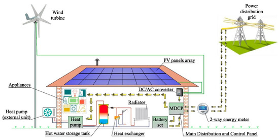
Figure 1.
Overall overview of the systems.
Figure 2 represents the framework of the created system.
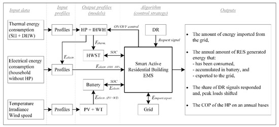
Figure 2.
System framework of the smart active residential building home energy management system.
The first step “Input data” is dedicated to obtaining all the necessary data for creating models. In this step sets of raw data are being processed, and all errors eliminated.
When all raw data is already processed, the “Input profiles” that reflect particular time frames (necessary for the creation of the system components models) are created in Section 2.1.2 and Section 2.1.3.
In the third step, all necessary power output profiles and state of charge models are created using fundamental mathematical equations and specific methods (Section 2.1.4, Section 2.1.5 and Section 2.1.6).
This is followed by the control strategy (Section 2.2) which is, based on pre-set conditions of the created algorithm and input data, evaluates the ability of the system to respond to the DR signals requested, charge/discharge storages to its maximal/minimal levels, as well as to manage energy import/export to and from the grid.
In the final fifths step the results are obtained (Section 3).
2.1. Model Components
2.1.1. Input Data and Time Frames
Making an analysis of the measured data obtained from 25 buildings located in the Northern Jylland region of Denmark (i.e., electric power demand and thermal demand for space heating (SH) and domestic hot water (DHW)), an average statistical single-family detached household with the District Heating (DH) heat supply is chosen as a basis. The area of the household is around 120 sq. m.
Weather data (i.e., solar irradiance, wind speed, air temperature) were derived for the same location from two different sources, namely, the weather forecasting station based at Aalborg University laboratory, and the EnergyPRO software. The data from each source were carefully analyzed, compared, and some very minor errors were interpolated and eventually eliminated.
All data sets were selected for the same year (namely, 2013) and the same location (Nordjylland, Denmark). All the following input load profiles were created, and the simulations were executed with a time step of 15 min, and an observation period of one calendar year.
2.1.2. Household’s Thermal Load Profile
The study made by [24], covers almost 25% of the Danish building stock, where the combination of the district heating schemes and individual residential heat pumps in overall gradual expansion perspective offer the best solution to transform the residential heating sector towards reduced CO2 emission. It is assumed in this study, that DH network’s supply will be replaced with an individual HP in combination with HWST. Figure 3 illustrates the household’s total monthly (a) and an average daily (b) thermal energy consumption by highlighting shares of space heating and domestic hot water. The data show that the share of energy consumption directed on SH is significantly increased during the heating season (which lasts from 1 October to 30 April), while the DHW’s share is more or less stable throughout the year. The summarized numerical data are presented in Table 1.
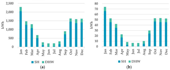
Figure 3.
Household’s thermal load profile: (a) Monthly consumption; (b) average daily consumption in specific months.

Table 1.
Household’s thermal load profile.
2.1.3. Household’s Electrical Load Profile
Figure 4 illustrates the household’s total monthly (a), and average daily (b) electrical energy consumption by highlighting the share of energy that has been consumed by the household itself (this load profile is taken as a basis, without any other electrical heating source, to execute all the following calculations) and the HP’s share (which is calculated using the algorithm, described in Section 2.2). Observed from the Figure 4 that the household’s consumption share (without HP) is mainly stable throughout the year (except February and March). While HP’s consumption is significantly increased during the heating season due to the high space heating demand and the numerical data are shown in Table 2.
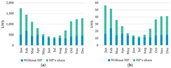
Figure 4.
Household’s electrical load profile: (a) Monthly consumption; (b) average daily consumption in specific months.
Table 2.
Household’s electrical load profile.
2.1.4. PV, WT, and Battery
The process of the creation of PV, WT power output profiles, as well as the SOC algorithm of the Li–Ion Battery storage is described in [27]. These models are taken as a basis. The size of renewable energy sources is chosen considering the ratio of maximum production for self-utilization and minimum energy excess (export to the grid), as well as the minimum shortage of energy (import from the grid). After analyzing a dozen scenarios combining different sizes of the PV array and WT, the best combination in terms of the optimal amount of imported and exported energy from/to the grid is chosen as follows. Table 3 and Table 4 below summarize the parameters of the PV arrays and WT such as rated power, size, efficiency, that have been used to create a building model.
Table 3.
Photo voltaic (PV) panel parameters 1.
Table 4.
Water Tank (WT) parameters 1.
Three different capacity of battery storage is compared. As demonstrated in [28] a typical size of a backup battery for domestic application is in a range of 4.5–12 kWh. The rated power and the energy capacity of the smallest size battery are chosen with respect to a maximal peak demand of the household without HP application and are considered as a scenario, just to visually examine how the size of the battery may affect the results. No specific criteria are applicable in this case. The medium-size battery is chosen considering the ability to accommodate maximal peak power production from RESs (both PV arrays and WT,) during one hour. The rated power of the largest size battery is chosen to meet the maximal peak power demand of the household (incl. HP), and the rated energy capacity is selected to provide one hour of islanded off-grid power supply for the household in these conditions. Table 5 summarizes the parameters for all three batteries. The round-trip efficiency, calendar ageing (degradation), and self-discharging per hour are neglected in this study. It is assumed that the efficiency of charging and discharging cycles is constant 100% despite the fact that this coefficient varies between 75–77%, according to [29]. A more detailed justification of such neglect will be provided in the results and discussion sections.
Table 5.
Battery parameters.
2.1.5. HP, IHWH, and HWST
In residential sector, heat pumps are used to fulfill building’s heat demand by transferring thermal energy from an external low-temperature renewable heat source such as ambient air, ground, fresh or seawater to higher temperature useful for space heating and/or domestic hot water (which are in most cases water or in-building air). The transferring process is realized by evaporating, compressing, condensing and expansion of the working fluid (refrigerant liquid).
A basic vapor compression heat pump cycle is realized as follows. The working fluid, turning itself into a gas within the “evaporator”, absorbs the heat from the external low-temperature heat source (the evaporator, in this case, works as a first heat exchanger). The compressor then raises up the pressure of the gas, increasing thereby its temperature. The hot gas, flowing through “condenser” and being hotter than the secondary source (water or in-building air), dissipates its heat to this source and condenses thus back into a liquid (the “condenser coils”, in this cycle, work as a second heat exchanger). The liquid finally flows back through the expansion valve, reducing thus its pressure and cooling down, then, enters back the evaporator, turning itself again into gas, and the cycle repeats. Figure 5 demonstrates a general overview of the heating system in the household, including the heat pump’s cycle.
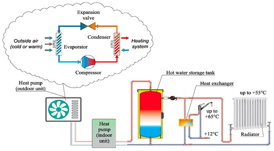
Figure 5.
Overall overview of the household’s heating systems.
This paper investigates the capabilities of an electrically driven air-to-water type vapor compression heat pump for heating application consisting of two units:
- Compact mono-block indoor unit with circulation pump, three-way diverter valve (heating/DHW heating), instantaneous heating water heater, control unit, and
- Outdoor unit that contains evaporator, compressor, condenser, diverter and expansion valves, and variable speed fans. The HP is considered with output-dependent/inverter-controlled scroll type compressor (that uses an external variable-frequency drive to control the speed).
The size of the heat pump was chosen considering the average ambient temperature during the heating season +3.8 °C, the water flow temperature limit +65 °C, and the average household’s thermal demand during the heating season 2.1 kW. The rated electric power of the HP was selected considering manufacturers technical data as reference information (to narrow the range), however, the COP, as well as thermal energy output and electrical energy input were calculated using the equations and the algorithm below. In order to cover household’s maximal thermal peak demand (i.e., 11.5 kW) and to supply the heat outside HP’s working temperature limits an instantaneous heating water heater (IHWH) with the rated power of 6 kW and a buffer thermal storage (viz. HWST) is applied. The HP’s parameters containing rated electrical power, air intake working temperature limits, the secondary circuit water flow temperature limit are derived from the Viessmann’s technical guide paper [30] and are shown in Table 6.
Table 6.
Heat pump (HP) parameters.
Thermal power output from the HP is calculated, using following equation:
where: —rated electric power, (kW), —coefficient of performance or, in other words, transformation coefficient from electrical to thermal energy, —time step (which is 0.25 h in the current model).
The maximal theoretical COP is determined by the inverse Carnot efficiency [31]. The Carnot cycle demonstrates an ideal process of energy transformation, however, taking into account performance and efficiency of different components, declared by a variety of manufacturers, such as compressor (hermetically sealed scroll, oiled/dry, frequency/inverter-controlled types), different coatings of evaporator, fans, circulation pumps, valves, working liquids, and losses appeared during operation, this cycle becoming far from ideal. The empirical examination results provided by [32] demonstrates corresponding real COP for different types of HPs. M. Bruner at al. in their study [33] show that for air to water types HP an averaged empirical factor (which is deviation from the ideal Carnot cycle incl. all losses) is equal to 0.38. Thus, the practical COP is calculated by the equation below:
where: —Carnot efficiency, —outlet (flow) water temperature (K), —inlet air temperature (K), —time step (hour), —deviation factor from the ideal Carnot cycle (dimensionless).
If the heat pump cannot meet the heat demand in mono mode, or when the ambient temperature falls to near or below freezing, the condenser is in a very big risk of being icing up, causing significant damage to the heat pump. To meet the heat demand, the HP must be operated in mono energetic mode (with instantaneous heating water heater), and to prevent potential condenser icing up, the defrost mode must be operated. The defrost mode plays a very important role in HP’s operation process, and can significantly reduce the household’s heat supply by distributing a great share of the total heat produced to melt the frost appeared on the external condenser coils. A detailed explanation of this process is presented in [34]. In this model, the defrost cycle is implemented by turning it “ON” for 5 min hourly. The annual share of thermal energy spent on defrosting, as well as electrical energy consumption share, will be presented in the result section.
To protect the compressor from high pressure caused by the change in the flow of refrigerant at the reversing valve, a five-minute starting time delay is introduced. Thus, having a model with a 15 min time step, the energy output for each first HP’s “ON” loop will be counted for the rest 10 min only. Accordingly, thermal energy outputs, incl. delay time and defrost time are calculated by the following equations.
where: —thermal power output, (kW), —time step (h), , —time reduction coefficients (that are equal to in this model, dimensionless).
The literature demonstrates various heat storage technologies [35]. A comparison of active and passive storage technologies (namely, the storage tank and the building’s thermal mass) is presented in [36]. Even though building’s thermal mass can offer a better cost-effective solution (based on the mentioned-above comparison results), this study is devoted to the most commonly used HP’s system for domestic application nowadays—the hot water storage tank (HWST) [2,37]. A variety of HWST models have been presented in many studies. A few examples can be found in [33,38,39].
In this model, the thermal energy capacity of the HWST (kWh) is calculated using the specific heat conversion equation [31]:
where: —heat capacity of water (J/kg⋅°C), —mass (kg), —temperature difference (°C), —volume (m3), —density of water (kg/m3).
As one can see from the above equation, the decision-making parameters are temperature and volume. It is considered that the minimum possible cold-water inlet temperature is +12 °C, while the outlet (flow) water temperature is +65 °C (see Figure 5). These temperature indicators are considered as set points for calculating energy capacity.
The model of HWST in this case study has been created without taking into consideration the stratification (neither highly nor moderately), as well as thermal cline effect as described in [37]. It is assumed that water inside the storage tank is constantly mixed and the temperature is uniform. The controlled (min/max) hot water temperature boundaries of the HWST are set in the range from +55 °C to +65 °C. Thus, using the Equation (6) difference is 10 °C for this volume and is equivalent to 5.8 kWh of thermal energy. When the temperature increases from +12 °C to +65 °C, water accumulates 30.8 kWh of thermal energy (for 0.5 cubic meter tank. See Table 7 below). It is also a fairly obvious phenomenon, that thermal storage loses some part of energy over a period of time. In this study, it is assumed that HWST loses one percent of its State of Energy per every 24 h (or 1/24 percent per hour). Thus, the amount of thermal losses in this model for each time step is calculated by the equation below.
where: —state of energy of the HWST for each time step (kWh), —time step (h).
Table 7.
Hot water storage tank (HWST) parameters.
The State of Energy of the HWST for each time step t is calculated using the following approach.
where: —initial state of energy of the HWST (kWh), —thermal energy output from the heat pump (kWh), —thermal energy consumption of the household (kWh), —thermal energy losses of the HWST (kWh), —time step (h).
The electrical energy consumption, based on the SOE of HWST, household’s thermal demand and HWST’s losses for each time step will finally be converted back using the equation below.
Three different volumes and, accordingly, energy capacity scenarios of the HWST are evaluated in this study. Namely, 0.25, 0.5 and 1 cubic meter hot water storage tanks. Since theoretically, the flow water temperature within the HWST cannot fall below +12 °C (it is assumed that the HWST is placed in-house with higher space air temperature), and consequently, no thermal energy can be extracted from the water below this limit, the parameters will look as follows. Table 7 represents energy capacity and its percentage equivalent in relation to the temperature difference for the three HWST volume scenarios.
The amount of thermal energy controlled in kWh and it’s equivalent in reserve hours provided, as well as the amount of energy lost will be presented for each scenario in Section 3 (Results).
2.1.6. Demand Response Signal
Artificial DR request signal is simulated following the logic below. Analyzing the electricity balance data provided in public by [40], it is investigated that, as of 2018, Denmark’s Annual Gross Consumption (i.e., the sum of the consumption incl. transmission loss) is 34,168 GWh, the highest hourly peak load is 6089 MWh, while an average hourly demand is 3900 MWh. Thus, the highest peak-hour demand in Denmark appearing during a year is 56% higher than the average hourly demand.
Taking into account the hourly consumption profile and the annual mean value, the number of appearances above the mean value in each particular hour of a day during a year has been investigated and counted (e.g., 300 times from total 365 days has appeared at 17:00, and 298 times out of 365 days at 18:00). The percentages of the appearance of average consumption are presented in Figure 6a.
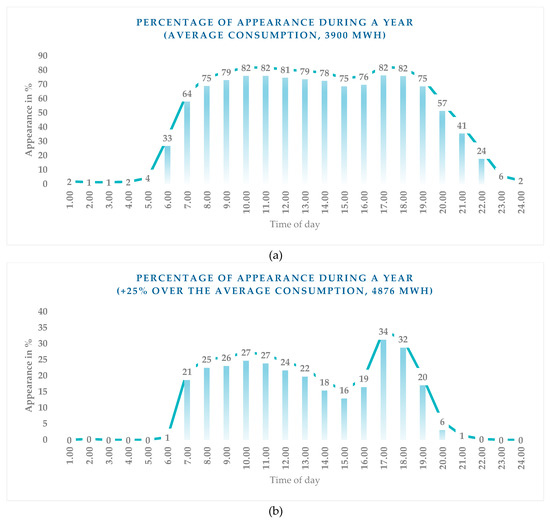
Figure 6.
Peak hours distribution curve of Denmark’s electricity grid in 2018: (a) average consumption; (b) 25 percent over the average limit.
In the next step, it was decided to increase the limit to 25% above the annual mean value and then it gives the percentages of appearance of the value that is greater or equal to 4876 MWh. The results are shown in Figure 6b.
The case with the limit set to 25% above yearly mean value is used in the rest of the paper, as an example for peak shaping. This value might be a realistic threshold for the future application of demand response depending on actual local conditions for transformer loading, line loading etc. However, the method set up here can be applied for any chosen limit, so this is just to be seen as an example. Based on the above, it is decided to simulate the DR request signals using random distribution function with percentage probability shown in the case (b). According to that, having one-year model with 35,040 (15-min) time steps, 4668 DR request signals were simulated.
2.2. Control Strategy
The control strategy is organized as follows. Figure 7 and Figure 8 below should be considered as two inseparable components of hybrid energy flow and control algorithm for energy management of active buildings. Based on the initialized weather forecast data and the created power output models of renewable energy sources, the energy derived from the PV arrays and WT during a first 15-minute time step period is calculated. The energy produced by RESs will be consumed by the household and the heat pump as a first priority step. These two blocks are shown separately due to fact that the household’s consumption is considered as fixed (i.e., uncontrollable) in this case study, and the main flexibility is obtained from the second, red outlined, block, the HP. Following the conditions shown in Figure 8 (such as working temperature limits, SOE of the HWST, defrost mode and the availability of the DR request signals), the HP and an additional heat source can be turned either ON or OFF. The total electrical energy consumption is then summarized and subtracted from RES calculated value. The excessive RES energy production (if any) will, depending on the SOC of the battery, either be accumulated in the battery (as a second priority) or be exported to the grid. In the event of a shortage of on-site production, energy will be delivered from the grid based on the total consumption needs and state of charge as well. A detailed control strategy of RESs utilization, the SOC of the battery storage, charge/discharge schedule managing, and the grid import/export power, including all equation, is described in [31].
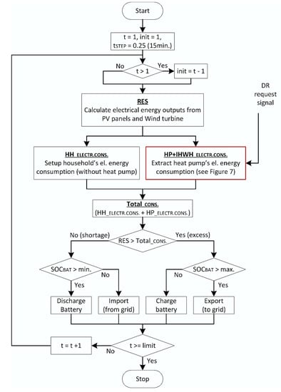
Figure 7.
The flowchart represents a general overview of the energy flow of the created model, as well as the simplified battery state of charge (SOC) control algorithm in active buildings.
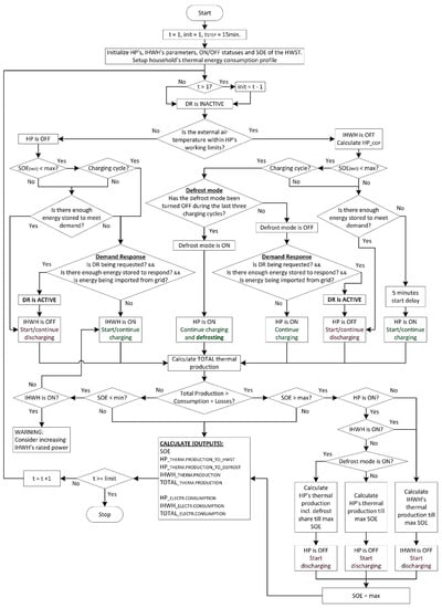
Figure 8.
Combined flowchart for energy management of the HP, IHWH, and the state of energy of the HWST, including the demand response application in active buildings.
3. Results
The results shown in Table 8, Figure 9, and Table 9 represent the performance of the integrated thermal energy system. Table 8 shows energy data and the performance of HWST, namely a number of backup heat supply hours that HWST can provide within the controlled temperature boundaries for three different volume scenarios (0.25, 0.5 and 1 cubic meter), as well as the amount of energy which is lost within the HWST during a year.
Table 8.
Ability of the HWST to accumulate thermal energy.
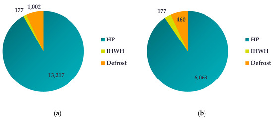
Figure 9.
The performance of the heat pump with medium size HWST (without demand response (DR) application) on an annual basis: (a) Thermal energy production, kWh; (b) electrical energy consumption, kWh.
Table 9.
Thermal system performance on an annual basis without and with DR application.
A ratio of the thermal energy produced, and electrical energy used to produce this thermal energy (by the HP and an IHWH) on an annual basis, as well as shares of energies spent for defrosting cycle (which is highly important to operate the HP technologically properly, but can be said wastefully for household’s needs), as a performance indicator, are illustrated in Figure 9a,b. It is observed, for the production of 13,217 kWh of heat, 6063 kWh of electricity have to be used, thus, in accordance with Equation (1) the annual COP of the HP is equal to 2.18, while the share of 7,6% of the total thermal energy produced (namely 1002 kWh). As well as electrical energy used (namely 460 kWh), was spent on defrosting, which is a rather wasteful amount. At the same time, the very insignificant amount of 177 kWh of electrical energy used by the IHWH, indicates that the HP covers most of the heat demand (i.e., 97%) in mono mode and that the size of the HP is chosen properly.
A comparison of two different scenarios (namely without and with DR application) for three different HWST’s volumes using the same data indicators are summarized in Table 9 to analyze the deviation and to investigate the DR impact on final performance. The results show that the DR application has no impact on overall performance (the HP’s COP is equal to 2.18 in all cases). However, the smaller size of the HWST, the more energy is used by IHWH, which generally means that the small volume of the HWST is insufficient to support HP to cover the heat demand in mono mode for a long time, thus IHWH turns ON more frequently and the total COP decreases.
The curves that demonstrate the maximum and average values of the power produced by the PV array and the WT, as well as total energy produced during particular months are given in Figure 10a–c. Having 3.15 kW rated power of the PV array and 6 kW rated power of the WT, it is observed (Figure 10a) that PV production has not reached its maximum power output throughout the year (showing its maximum of 2.6 kW in the late spring and summertime), while the WT’s power output of 6 kW observed very often due to windy weather condition in Denmark (see Figure 10b). Figure 10c illustrates the pre-dominant PV production in the summer, and early autumn seasons, while the share of WT prevails in the rest of the year. Nevertheless, the low total RES production (which is due to the weather conditions) is observed in the period of September–November, January–February, and a high production is observed in a period of March–August and December. It is expected that this discrepancy will be compensated by the battery and the energy import from the grid.
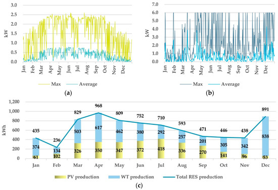
Figure 10.
Power output profiles of the renewable energy sources: (a) PV array power output profile; (b) wind turbine power output profile; (c) total RES energy production.
The utilization of the renewable energy produced on-site, renewable energy exported, and the grid imported energy (which are, to a greater extent, affiliated with the size and efficiency of the battery, as well as the presence of load at a specific time) is demonstrated for two different battery and HWST scenarios in Figure 11a,b below. A large energy import from the grid is observed between September and April (which is mainly due to a shortage of RES energy production and high demand, as shown in Figure 4a and Figure 10c above), while export of energy is observed in a period of March - August and December. This phenomenon can be explained as an excess of RES production and low demand in the summertime, as well as the insufficient battery storage capacity in both scenarios.
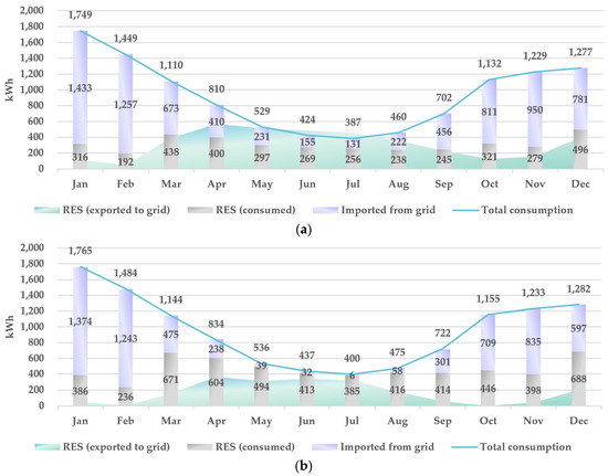
Figure 11.
RES energy utilization and the exchange with the grid: (a) scenario with the smallest battery and the smallest HWST’s size; (b) scenario with the largest battery and the largest HWST’s size.
One of the interesting findings by making an analysis of results obtained from 24 simulations is the difference between values of total annual energy imported from the grid under various battery scenarios. Regardless of all expectations and more than a double difference in the battery size, the difference between the above values is very small (Figure 12 and Table 10 below). Figure 12 demonstrates the shares of energy (namely imported from the grid and RES generated), which are utilized to meet the household’s demand in four scenarios. The discrepancy between scenarios with battery 1 and battery 3 in each case is in the range of 2–4%. That basically means, that regardless of the size of the battery (of course, on a reasonable scale), it cannot provide long-term energy compensation, mainly due to the fact that there are still many periods during a year where total RES generation (from both PV and WT) is very low or absent at all (mostly in January and February), and that the largest battery, in this case-study, helps to utilize only 16% more RES generated energy comparing to the scenario without battery at all.
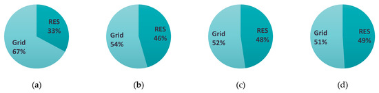
Figure 12.
Household’s demand coverage shares for different battery scenarios and the medium HWST’s size, where: (a) No battery; (b) battery 1; (c) battery 2; (d) battery 3.
Table 10.
Comparison table of RES consumed, battery utilized, and grid exported/imported energy values, obtained as a result of simulating different scenarios.
Another interesting fact is that the use of the DR has no influence on the final annual consumption as well as the amount of energy imported from the grid. As an example, the total energy consumption in the scenario with 0.25 m3 HWST without DR application is 11,246 kWh, while in the same HWST scenario with DR application; it is 11,258 kWh (see Table 10 below for more results). The discrepancy in result values between “without” and “with” DR application is less than 0.2% which is completely negligible. That one more time proves the fact that the DR application does not harm the user preferences and the user will not pay more. The values for on-site RES produced energy, including consumed by household, passed through the battery (i.e., charged/discharged), exported to the grid, and the values for energy imported from the grid are summarized for 24 different cases (comparison of the HWST, battery size, and DR application) in Table 10.
Figure 13a,b illustrate the application of the energy management without (a) and with (b) DR. The fourth day of the simulation (4th of January) with the largest HWST (i.e., 1 m3) and a medium-sized battery (battery Scenario 2, i.e., 8 kWh) is presented. Even though the cycles were shifted during the first three days due to DR, these two figures can ideally represent most of the processes of the created model. The attention should mainly be focused on the period between 05:30–11:00 (Figure 13a).
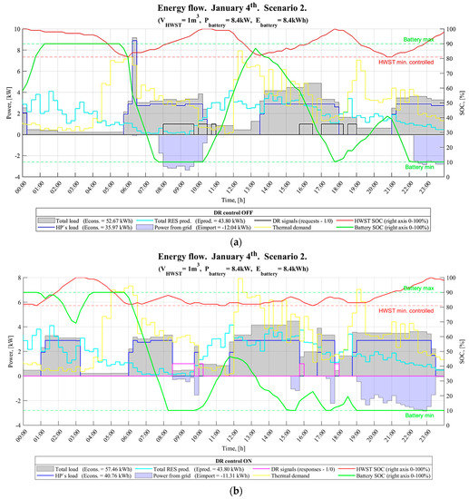
Figure 13.
Energy flow model simulation result for one day: (a) Without responding to DR request signals; (b) with DR control activated.
As can be seen at 05:45, the level of thermal energy of HWST had reached a minimum level. To meet the household’s heat demand, the heat pump was turned ON, thus starting the charging cycle of the HWST. Having very high thermal demand, as of 06:15, HP’s production became insufficient in mono mode, and IHWH as an additional heat source was turned ON, and, thereby the peak demand occurs. Since the battery SOC was at its maximum at 05:30 and the RES production was very low, it is observed that the total load (including a peak value) was fully covered by the battery itself for two hours.
As one can see at 07:45, the battery SOC reached a minimum level, and since RES production was still very low, import appeared. Based on the work performed in Section 2.1.6 above, a series of DR request signals were received between 08:00–11:00. Since, as of 08:30, the HWST had become half-charged, having sufficient amount of thermal energy to cover the heat demand, as well as meeting all other conditions (described in the algorithm in Figure 8, Section 2.2), the system responded to the received DR signal by turning off the heat pump (see 10:30 in Figure 13b). The same figure also shows that almost all of the energy imported between 07:45–10:30 was shifted to the evening time after 19:00.
Table 11 below shows the percentage of DR responded signals for different battery and HWST scenarios. The results show that the bigger the battery size the lower the percentage. As an example, battery 1 (under scenario with 0.25 m3 HWST) shows 10.8%, while battery 3–10.1%. This can be explained by the fact that the battery covers a certain number of peak loads, and the share of power taken from the grid at that particular time (when the signal is requested) is very insignificant or does not exist at all. Thus, scenarios without the battery, in general, demonstrate much larger responsiveness, namely: 14.8% of DR requested signals were responded under the scenario with 0.25 m3 HWST, while the maximal flexibility of 22.3% was reached in the scenario with the largest HWST volume (i.e., 1 m3).
Table 11.
The peak loads shifting potential of the proposed model, namely, the number of DR signals requested and the share of responses compared for three different HWST’s volumes and three battery capacity scenarios on an annual basis.
4. Discussion
The graphical and numerical results obtained in Section 3 show that the proposed model can be successfully applied to estimate energy activity and flexibility range in smart active residential buildings, combining different system components within one hybrid energy flow and management algorithm.
The main advantage of this study compared with other works analyzed in Section 1 is that the model combines a larger number of system components within a single energy management algorithm, as well as demonstrates more accurate results based on Matlab models and simulation, comparing to theoretical calculations of the flexibility that can be achieved (using fundamental equations) as shown in [20].
The limitation inherent in some components of the created model in terms of accuracy (namely, the battery efficiency, which is neglected in this study), can be overcome by applying more advanced and accurate methodologies. An overview of the various estimation technics can be found in [41], whereas the application example in [42]. Since the creation of a very detailed battery model was not targeted in this study, a simple approach in Matlab is utilized. Nevertheless, based on the results shown in Section 3 (Figure 10 and Figure 11, and Table 10) it is clearly observed, that even having a very large battery and 100% round trip efficiency—it does not make a very big influence on the amount of energy imported from the grid compared to a scenario without battery at all (for Danish conditions). One may say that the sizes of RESs are insufficient, however, the sizes of PV and WT were also selected based on a comparison of the results of more than 20 different simulations, considering import and export indicators as the main criteria. With the simultaneous increase in both RES and battery size to the enormously and unreasonably large for the household, export significantly increases in the summertime (mainly due to lack of demand), while leaving a fairly large share of import between autumn and early springtime (due to high demand and periods of adverse weather conditions for the RES production), which gives reason to draw such a conclusion.
From the other side, the percentage of flexibility obtained varies from 10–22%, which is quite satisfying results, considering the fact that DR response is applied only to very specific conditions focused on the user’s comfort preferences. Even though the share of DR responded signals are bigger in a scenario without battery, the fact of the presence of battery, in this case, plays opposite role. The larger battery size, the less energy imported from the grid, and the fewer request signals have to be responded.
If to assume that the critical load limit, described in Section 2.1.6, would increase to 35% above the annual mean value equal to 5266 MWh, then the number of DR request signals will be much less, since fewer periods will appear above this limit. This will definitely lead to the fact that the total amount of energy shifted per year will be also much less. However, the percentage of flexibility, in general, should not differ significantly from the results obtained in this study (initially, due to the given conditions of the created algorithm). It would also be interesting to investigate the model behavior and the amount of energy shifted under the local 10/0.4 kV grid conditions (that has fairly different peak load hour curve), and to compare the difference between two cases, however, this is the subject of another study.
The created model and simulation results show that having such integrated systems and the demand response application may lead to techno-economic benefits for both household’s owners, in terms of sustainability and reducing the cost of energy, as well as the DSO’s in terms of obtaining certain percent of the flexibility on demand-side and hence the ability to reduce peak loads thus making grid operation process smoother.
Future research work will focus on investigating the actual amount of energy shifted (in kWh) on an annual basis, as well as on forecasting amount of flexibility that can be achieved. In order to do so, a price, as well as a specific statistical model for forecasting, should be introduced. This will follow with the aggregation of a group of such kind of buildings.
5. Conclusions
In this paper, the energy flow model of a domestic dwelling consisting of PV array, individual on-site wind turbine, battery storage, a heat pump in combination with HWST was created. Three different scenarios of the battery, three scenarios of the HWST, as well as two scenarios of the DR application (i.e., “with” and “without”) were simulated. The paper assesses the flexibility for each scenario, and the results were summarized and compared in detail.
Results imply that the heat pump, without jeopardizing any user comfort preferences, even with the smallest thermal storage size (i.e., 0.25 m3) and without battery provides quite satisfied load shifting flexibility for this condition, namely 14.8% (Table 11 above). However, the battery seems not to be very efficient in northern climate conditions by showing the performance that does not exceed 16% in terms of RES energy conservation (Figure 12 above).
Considering still very high investment cost of lithium–ion batteries and a very poor price of energy exported to the grid in Denmark (from RES energy trading point of view), a more reasonable and forward-looking solution for the RES energy utilization for household owners (instead of rising up the size of the battery) could be found in the following combination. A small battery can be used for the short-term (hourly) energy compensation, a large HWST for the provision of the demand energy flexibility services, and an electrolyzer coupled with fuel cells that stores energy in a form of pressurized hydrogen and oxygen for the storage of large quantities of energy for a long period. The energy can then be used by a hydrogen car or converted back into electricity by fuel cells. However, to evaluate the profitability of such a combination, a more comprehensive techno-economic analysis has to be executed.
Despite the results obtained in this study, the battery may still be more attractive in other locations with different RES generation and power demand patterns, as well as based on benefits provided from the network side.
Author Contributions
Investigation, conceptualization, methodology, writing—original draft, V.S.; supervision, review & editing, J.R.P., B.B.-J.; review & editing, S.P.
Funding
This research received no external funding.
Acknowledgments
The authors kindly acknowledge the editor and two anonymous reviewers for helpful observations and comments, which have helped to improve an earlier version of this manuscript.
Conflicts of Interest
The authors declare no conflict of interest.
Nomenclature
| Acronyms | |
| BEMS | Building Energy Management System |
| CO2 | Carbon dioxide |
| COP | Coefficient of Performance |
| DC/AC | Direct Current/Alternating Current |
| DH | District Heating |
| DHW | Domestic Hot Water |
| DR | Demand Response |
| DSO | Distribution System Operator |
| EMS | Energy Management System |
| EPBD | Energy Performance of Buildings Directive |
| EU | European Union |
| GBC | Green Building Council |
| HAWT | Horizontal Axis Wind Turbine |
| HH | Household |
| HP | Heat Pump |
| HWST | Hot Water Storage Tank |
| IHWH | Instantaneous Heating Water Heater |
| LEED | Leadership in Energy and Environmental Design |
| MDCP | Main Distribution and Control Panel |
| nZEB | nearly Zero Energy Building |
| PV | Photovoltaic |
| RES | Renewable Energy Source |
| SH | Space Heating |
| SOE | State of Energy |
| SOC | State of Charge |
| WT | Wind Turbine |
| bat. | Battery |
| cons. | Consumption |
| el. or electr. | Electrical |
| init. | Initial |
| prod. | Production |
| therm. | Thermal |
| Symbols, Descriptions and Units | |
| Heat capacity of water (J/kg⋅°C) | |
| Theoretical (ideal) coefficient of performance (dimensionless) | |
| Coefficient of performance of the heat pump at a particular time (dimensionless) | |
| Ebattery | Rated energy capacity of the battery (kWh) |
| Econs. | Electrical energy consumption over a period of time (kWh) |
| Eimport. | Electrical energy imported from the grid over a period of time (kWh) |
| Eprod. | Electrical energy produced over a period of time (kWh) |
| Electrical energy consumption of the heat pump at a particular time (kWh) | |
| HH_ELECTR.CONS. | Electrical energy consumption of the household at a particular time (kWh) |
| HP’s load | Electric power demand of the heat pump (kW) |
| Deviation factor from the ideal Carnot cycle (dimensionless) | |
| Mass (kg) | |
| Carnot efficiency (dimensionless) | |
| Density of water (kg/m3) | |
| Pbattery | Rated power of the battery (kW) |
| Thermal power output from the heat pump at a particular time (kW) | |
| Rated electric power of the heat pump at a particular time (kW) | |
| Thermal energy consumption of the household (kWh) | |
| Thermal energy output from the heat pump at a particular time (kWh) | |
| Thermal energy output from the heat pump at a particular time including starting delay (kWh) | |
| Thermal energy output from the heat pump at a particular time directed on defrosting the external coil (kWh) | |
| Thermal energy capacity of the hot water storage tank (kWh) | |
| Thermal energy lost in a hot water storage tank over a period of time (kWh) | |
| State of charge of the battery at a particular time (%) | |
| State of energy of the hot water storage tank at a previous moment of time (kWh) | |
| State of energy of the hot water storage tank at a particular time (kWh) | |
| Initial state of energy of the hot water storage tank (kWh) | |
| t | Time step (h) |
| , | Time reduction coefficients (dimensionless) |
| Outlet (flow) water temperature (K) | |
| Inlet air temperature (K) | |
| Temperature difference (°C) | |
| or VHWST | Volume of the hot water storage tank (m3) |
References
- Lund, H.; Kempton, W. Analysis: Large-Scale Integration of Renewable Energy—Chapter 5. In Renewable Energy Systems: A Smart Energy Systems Approach to the Choice and Modeling of 100% Renewable Solutions, 2nd ed.; Elsevier Inc.: Amsterdam, The Netherlands, 2014; pp. 79–129. [Google Scholar]
- Fischer, D.; Madani, H. On heat pumps in smart grids: A review. Renew. Sustain. Energy Rev. 2017, 70, 342–357. [Google Scholar] [CrossRef]
- Lund, P.D.; Lindgren, J.; Mikkola, J.; Salpakari, J. Review of energy system flexibility measures to enable high levels of variable renewable electricity. Renew. Sustain. Energy Rev. 2015, 45, 785–807. [Google Scholar] [CrossRef]
- Weitemeyer, S.; Kleinhans, D.; Vogt, T.; Agert, C. Integration of Renewable Energy Sources in future power systems: The role of storage. Renew. Energy 2015, 75, 14–20. [Google Scholar] [CrossRef]
- Herter, K. Residential implementation of critical-peak pricing of electricity. Energy Policy 2007, 35, 2121–2130. [Google Scholar] [CrossRef]
- Triki, C.; Violi, A. Dynamic pricing of electricity in retail markets. 4OR 2009, 7, 21–36. [Google Scholar] [CrossRef]
- Allcott, H. Rethinking real-time electricity pricing. Resour. Energy Econ. 2011, 33, 820–842. [Google Scholar] [CrossRef]
- Albadi, M.H.; El-Saadany, E.F. Demand response in electricity markets: An overview. In Proceedings of the 2007 IEEE Power Engineering Society General Meeting, PES, Tampa, FL, USA, 24–28 June 2007. [Google Scholar]
- Ram, M.; Bogdanov, D.; Aghahosseini, A.; Gulagi, A.; Oyewo, S.A.; Child, M.; Fell, H.-J.; Breyer, C. Global Enercy System Based on 100% Renewable Energy—Power Sector; Lappeenranta University of Technology: Lappeenranta, Finland; Energy Watch Group: Berlin, Germany, 2017. [Google Scholar]
- European Commission. DIRECTIVE 2010/31/EU OF THE EUROPEAN PARLIAMENT AND OF THE COUNCIL of 19 May 2010 on the energy performance of buildings (recast). Off. J. Eur. Union 2010, 53, 13–35. [Google Scholar]
- Gynther, L.; Lapillonne, B.; Pollier, K.; Bosseboeuf, D. Energy Efficiency Trends and Policies in the Household and Tertiary Sectors (ODYSSEE-MURE Project); ADEME: Montpellier, France, 2015. [Google Scholar]
- European Commission. DIRECTIVE (EU) 2018/844 OF THE EUROPEAN PARLIAMENT AND OF THE COUNCIL of 30 May 2018 amending Directive 2010/31/EU on the Energy performance of buildings and Directive 2012/27/EU on energy efficiency (factsheet attachment). Off. J. Eur. Union 2018, 61, 1. [Google Scholar]
- European Commission. DIRECTIVE 2012/27/EU OF THE EUROPEAN PARLIAMENT AND OF THE COUNCIL of 25 October 2012 on energy efficiency, amending Directives 2009/125/EC and 2010/30/EU and repealing Directives 2004/8/EC and 2006/32/EC. Off. J. Eur. Union 2012, 55, 1–56. [Google Scholar]
- European Commission. DIRECTIVE (EU) 2018/844 OF THE EUROPEAN PARLIAMENT AND OF THE COUNCIL of 30 May 2018 amending Directive 2010/31/EU on the Energy performance of buildings and Directive 2012/27/EU on energy efficiency. Off. J. Eur. Union 2018, 61, 75–91. [Google Scholar]
- Riffonneau, Y.; Bacha, S.; Barruel, F.; Ploix, S. Optimal power flow management for grid connected PV systems with batteries. IEEE Trans. Sustain. Energy 2011, 2, 309–320. [Google Scholar] [CrossRef]
- Kuzlu, M.; Pipattanasomporn, M.; Rahman, S. Hardware demonstration of a home energy management system for demand response applications. IEEE Trans. Smart Grid 2012, 3, 1704–1711. [Google Scholar] [CrossRef]
- Lopes, R.A.; Chambel, A.; Neves, J.; Aelenei, D.; Martins, J. A Literature Review of Methodologies Used to Assess the Energy Flexibility of Buildings. Energy Procedia 2016, 91, 1053–1058. [Google Scholar] [CrossRef]
- Hewitt, N.J. Heat pumps and energy storage—The challenges of implementation. Appl. Energy 2012, 89, 37–44. [Google Scholar] [CrossRef]
- Halvgaard, R.; Poulsen, N.K.; Madsen, H.; Jørgensen, J.B. Economic Model Predictive Control for building climate control in a Smart Grid. In Proceedings of the 2012 IEEE PES Innovative Smart Grid Technologies (ISGT), Washington, DC, USA, 16–20 January 2012; pp. 1–6. [Google Scholar]
- Six, D.; Desmedt, J.; Bael, J.V.A.N.; Vanhoudt, D. Exploring the Flexibility Potential of Residential Heat Pumps. In Proceedings of the 21st International Conference on Electricity Distribution, Frankfurt, Germany, 6–9 June 2011; pp. 6–9. [Google Scholar]
- Oldewurtel, F.; Ulbig, A.; Parisio, A.; Andersson, G.; Morari, M. Reducing peak electricity demand in building climate control using real-time pricing and model predictive control. In Proceedings of the 49th IEEE Conference on Decision and Control (CDC), Atlanta, GA, USA, 15–17 December 2010; pp. 1927–1932. [Google Scholar]
- Tahersima, F.; Stoustrup, J.; Meybodi, S.A.; Rasmussen, H. Contribution of domestic heating systems to smart grid control. In Proceedings of the 2011 50th IEEE Conference on Decision and Control and European Control Conference, Orlando, FL, USA, 12–15 December 2011; pp. 3677–3681. [Google Scholar]
- Andersen, P.; Pedersen, T.S.; Nielsen, K.M. Observer based model identification of heat pumps in a smart grid. In Proceedings of the 2012 IEEE International Conference on Control Applications, Dubrovnik, Croatia, 3–5 October 2012; pp. 569–574. [Google Scholar]
- Lund, H.; Möller, B.; Mathiesen, B.V.; Dyrelund, A. The role of district heating in future renewable energy systems. Energy 2010, 35, 1381–1390. [Google Scholar] [CrossRef]
- Mathiesen, B.V.; Lund, H.; Karlsson, K. 100% Renewable energy systems, climate mitigation and economic growth. Appl. Energy 2011, 88, 488–501. [Google Scholar] [CrossRef]
- Karlsson, K.; Balyk, O.; Zvingilaite, E.; Hedegaard, K. SDWS2011. 0809 District Heating Versus Individual Heating in a 100 % Renewable Energy System by 2050. In Proceedings of the 6th Dubrovnik Conference on Sustainable Development of Energy Water and Environment Systems, Dubrovnik, Croatia, 25–29 September 2011. [Google Scholar]
- Stepaniuk, V.; Pillai, J.; Bak-Jensen, B. Battery Energy Storage Management for Smart Residential Buildings. In Proceedings of the 2018 53rd International Universities Power Engineering Conference, UPEC 2018, Glasgow, UK, 4–7 September 2018. [Google Scholar]
- Fronius International GmbH. Creating a Green Future We Can Look Forward to. We Are Revolutionising the Energy Supply of the Future. Services and Product Programme 2017/18; Fronius International GmbH: Wels, Austria, 2017; Available online: https://docplayer.net/83575756-Creating-a-green-future-we-can-look-forward-to-we-are-revolutionising-the-energy-supply-of-the-future-services-and-product-programme-2017-18-years.html (accessed on 10 October 2018).
- Marczinkowski, H.M.; Østergaard, P.A. Residential versus communal combination of photovoltaic and battery in smart energy systems. Energy 2018, 152, 466–475. [Google Scholar] [CrossRef]
- Viessmann Werke GmbH & Co. KG. Technical Guide. VITOCAL Air/Water Heat Pumps; Viessmann Werke GmbH & Co. KG: Telford, UK, 2017. [Google Scholar]
- McGovern, J.A. Engineering Thermodynamics; Prentice Hall: New Jersey, NJ, USA, 1996. [Google Scholar]
- Wärmepumpen-Testzentrum Buchs (WPZ) and NTB Interstaatliche Hochschule für Technik Buchs. Test Results of Air to Water Heat Pumps Based on EN 14511: 2018/EN 14511: 2013/EN 14511: 2011/EN 14511: 2007/EN 14511: 2004/EN 14825: 2016 and EN 14825: 2013. Available online: https://www.ntb.ch/fue/institute/ies/wpz/pruefresultate-waermepumpen/ (accessed on 8 October 2018).
- Brunner, M.; Tenbohlen, S.; Braun, M. Heat pumps as important contributors to local demand-side management. In Proceedings of the 2013 IEEE Grenoble Conference, Grenoble, France, 16–20 June 2013. [Google Scholar]
- EnerGuide Natural Resources Canada’s Office of Energy Efficiency. Heating and Cooling With a Heat Pump; Natural Resources Canada’s Office of Energy Efficiency: Ottawa, ON, Canada, 2004. [Google Scholar]
- Parameshwaran, R.; Kalaiselvam, S.; Harikrishnan, S.; Elayaperumal, A. Sustainable thermal energy storage technologies for buildings: A review. Renew. Sustain. Energy Rev. 2012, 16, 2394–2433. [Google Scholar] [CrossRef]
- Hedegaard, K.; Mathiesen, B.V.; Lund, H.; Heiselberg, P. Wind power integration using individual heat pumps—Analysis of different heat storage options. Energy 2012, 47, 284–293. [Google Scholar] [CrossRef]
- Arteconi, A.; Hewitt, N.J.; Polonara, F. State of the art of thermal storage for demand-side management. Appl. Energy 2012, 93, 371–389. [Google Scholar] [CrossRef]
- De Coninck, R.; Baetens, R.; Verbruggen, B.; Driesen, J.; Saelens, D.; Helsen, L. Modelling and simulation of a grid connected photovoltaic heat pump system with thermal energy storage using Modelica. In Proceedings of the 8th International Conference on System Simulation, Liège, Belgium, 13–15 December 2010; p. 177. [Google Scholar]
- Mufaris, A.L.M.; Baba, J. Local control of heat pump water heaters for voltage control with high penetration of residential PV systems. In Proceedings of the 2013 IEEE 8th International Conference on Industrial and Information Systems, Peradeniya, Sri Lanka, 17–20 December 2013; pp. 18–23. [Google Scholar]
- Energinet. Electricity Balance Data. Available online: https://www.energidataservice.dk/da_DK/dataset/electricitybalance (accessed on 10 October 2019).
- Murnane, M.; Ghazel, A. A Closer Look at State of Charge (SOC) and State of Health (SOH) Estimation Techniques for Batteries; Analog Devices Inc.: Norwood, MA, USA, 2017; Available online: https://www.analog.com/media/en/technical-documentation/technical-articles/A-Closer-Look-at-State-Of-Charge-and-State-Health-Estimation-Techniques-....pdf (accessed on 10 October 2019).
- Jenkins, D.P.; Fletcher, J.; Kane, D. Model for evaluating impact of battery storage on microgeneration systems in dwellings. Energy Convers. Manag. 2008, 49, 2413–2424. [Google Scholar] [CrossRef]
© 2019 by the authors. Licensee MDPI, Basel, Switzerland. This article is an open access article distributed under the terms and conditions of the Creative Commons Attribution (CC BY) license (http://creativecommons.org/licenses/by/4.0/).