The Fast Discrete Tchebichef Transform Algorithms for Short-Length Input Sequences

Abstract

In this article, the fast algorithms for the discrete Tchebichef transform (DTT) are proposed for input sequences of lengths in the range from 3 to 8. At present, DTT is widely applied in signal processing, image compression, and video coding. The review of the articles related to fast DTT algorithms has shown that such algorithms are mainly developed for input signal lengths 4 and 8. However, several problems exist for which signal and image processing with different apertures is required. To avoid this shortcoming, the structural approach and a sparse matrix factorization are applied in this paper to develop fast real DTT algorithms for short-length input signals. According to the structural approach, the rows and columns of the transform matrix are rearranged, possibly by changing the signs of some rows or columns. Next, the matched submatrix templates are extracted from the matrix structure and decomposed into a matrix product to construct the factorization of an initial matrix. A sparse matrix factorization assumes that the butterfly architecture can be extracted from the transform matrix. Combining the structural approach with a sparse matrix factorization, we obtained the matrix representation with reduced computational complexity. Based on the obtained matrix representation, the fast algorithms were developed for the real DTT via the data flow graphs. The fast algorithms for integer DTT can be easily obtained using the constructed data flow graphs. To confirm the correctness of the designed algorithms, the MATLAB R2023b software was applied. The constructed factorizations of the real DTT matrices reduce the number of multiplication operations by 78% on average compared to the direct matrix-vector product at signal lengths in the range from 3 to 8. The number of additions decreased by 5% on average within the same signal length range.

1. Introduction

In recent years, discrete Tchebichef transform (DTT) became widely applied in image compression [1,2,3,4,5,6,7,8], video coding [8,9,10], signal processing [11], image segmentation [12], image denoising [13], speech recognition [14,15], etc. DTT is a linear orthonormal transform obtained from orthogonal Tchebichef polynomials. Compared with discrete cosine transform (DCT), DTT demonstrates similar energy compactness and decorrelation for images of nature scenes. Furthermore, DTT outperforms DCT in images with significant illumination variations. Owing to its energy compactness and decorrelation, DTT is extensively used and highly effective in image compression [1,2,3,4,5,6,7,8,16,17]. For example, in [10], the proposed DTT approximation was embedded in the software library x264 [18] for encoding video streams into the H.264/AVC standard [19]. It requires 38% fewer additions and eliminates bit-shifting operations compared to the 8-point integer approximation of the DCT currently used in H.264/AVC [20,21]. The latter requires 32 additions and 14 bit-shifting operations.

The signal processing in the DTT domain is applied in neural signal compression when the neural recording microsystems are designed with specific requirements for the power consumption, chip area, and the wireless interfacing data rate [22].

In [23], DTT was embedded in the wavelet-based still image coder SPECK. The resulting coder HLDTT has shown a significant improvement in peak signal-to-noise ratio at lower bit rates. Also, a reduction in encoding and decoding time over DCT-based embedded coders was achieved to realize a low-power image compression system for hand-held portable devices [7].

Other areas of DTT application are also of interest. In [24], a digital watermarking algorithm using DTT was proposed as more robust to Gaussian noise attacks. To add a watermark, the initial image is split into nonoverlapped blocks, and DTT is performed for each of them. A watermark image was embedded into the largest DTT coefficients of each block, resulting in time savings compared to DCT [24].

In various applications, reducing the computational time for DTT is essential for achieving real-time or high-performance implementations. The literature describes two primary types of DTT based on their applications: real DTT and integer DTT. The original real DTT matrix can be derived by multiplying each row of the integer DTT matrix by a specific coefficient. Consequently, fast algorithms for real DTT can be efficiently developed based on the fast algorithms designed for integer DTT [17].

Because the main application of DTT is image compression and video coding, the developing of fast DTT algorithms is oriented towards the standards of these applications. As a consequence, fast algorithms were constructed for the 4 × 4 and 8 × 8 two-dimensional (2D) integer DTT and its approximations [1,8,10,25,26,27,28,29,30,31,32,33]. The authors are not aware of any articles devoted to designing fast DTT algorithms for input sequences of lengths different from 4 and 8. However, along with image compression, DTT is utilized for various tasks such as signal and image denoising, segmentation, and classification, where the result is often affected by the size of the processing window. In these situations, restricting the window size to values of 4 and 8 is not relevant. Moreover, short-length DTT algorithms can be included as typical modules to develop long-length algorithms [34,35].

Therefore, an urgent problem is constructing fast DTT algorithms for short-length input sequences. Next, to determine the appropriate strategy for developing such fast DTT algorithms, the articles related to this problem are considered.

1.1. State of the Art of the Problem

To design fast DTT algorithms, the polynomial algebraic approach, sparse matrix factorization, and different heuristics are applied [22,25,26,27,28,29,30,31,32,33]. Recursive expressions for obtaining the entries for DTT matrices do not facilitate the development of fast radix-type algorithms, although such algorithms are efficiently and widely employed for orthogonal trigonometric transforms [36]. Thus, in [30], the polynomial algebraic approach is used to construct the fast algorithm for the 2D 4 × 4 real DTT. The expressions for transform matrix entries were regrouped to determine the products of Tchebichef polynomials via the linear combinations of new basis functions. These results reduce multiplications by 50% and additions by 31% compared to the naive product bearing in mind the separability and symmetry of the DTT matrix. However, very cumbersome mathematical calculations of the algebraic approach are an obstacle to obtaining fast algorithms for DTTs with other input sequence lengths.

In [1], multiplier-less algorithms were proposed for one-dimensional (1D) and 2D integer 8 × 8 DTTs. These algorithms were obtained heuristically, although they used butterfly architecture. The sparse matrix factorization or data flow graphs are not presented for them. Despite this, these algorithms are considered to be among the most effective. In the 1D case, the number of additions was reduced by 50% compared to a naive method when considering the separability and symmetry properties of the DTT. In addition, 29 shifts were required in the 1D case. However, the above heuristics were proposed to construct an algorithm specifically for the case of an 8 × 8 integer DTT. Generalization of it to cases of other lengths of data sequence was not considered.

The primary way to obtain fast DTT algorithms is sparse matrix factorization and/or construction of data flow graphs with butterfly architecture [28,29,30,31,32,33]. For example, in [28,29], sparse matrix factorization was proposed for a 4 × 4 real 2D DTT. Although an additional 20 shifts were required, it reduced multiplications by 81% and additions by 17% compared with the naive product bearing in mind the separability and symmetry of the DTT matrix. Proposed in [10], a fast algorithm with butterfly architecture for a 1D DTT approximation required only 20 additions, reducing operations by 55% compared to [1]. In [8], fast algorithms for 4 × 4 and 8 × 8 integer 1D DTTs were presented for data flow graphs based on butterfly architecture. The algorithms for 4 × 4/8 × 8 2D DTTs were also implemented using Verilog HDL [8].

Hence, efficient fast DTT algorithms are developed via sparse matrix factorization or data flow graphs with butterfly architecture. In general, such an approach is appropriate for designing fast DTT algorithms for even lengths of input sequences, including lengths different from 4 and 8. However, when dealing with odd lengths, problems arise in constructing butterflies, and thus the choice of an approach for constructing fast DTT algorithms for odd lengths remains open. Thus, the above short review of existing fast DTT algorithms allowed us to determine unsolved parts of the general problem of developing fast DTT algorithms for short-length input sequences.

1.2. The Main Contributions of This Paper

As previously mentioned, fast N-point DTT algorithms for short-length signals can be developed via data flow graphs with a butterfly architecture and sparse matrix factorization. However, for some values of N, constructing such architecture can be challenging. To address this shortcoming, we propose using the structural approach in addition to sparse matrix factorization to develop fast real DTT algorithms for short-length input signals. This approach was successfully applied to factorize the matrices of trigonometric transforms in [37,38,39,40]. As a result, the number of arithmetic operations for these transforms was significantly reduced. According to the structural approach, the rows and columns of the transform matrix are rearranged, possibly changing the sign of some rows or columns. Then, the predefined templates are searched and extracted from the transform matrix. Based on the predetermined factorization of templates, the factorization of the entire transform matrix is obtained.

The structural approach to DTT matrix decomposition is due to the symmetrical structure of the DTT coefficients matrix. However, as N increases, template extraction becomes a cumbersome process. That is why it is relevant to integrate the structural approach into the construction of data flow graphs with butterfly architecture. The efficiency of this trick owes to the symmetry of DTT coefficients, which can be paired for constructing butterfly modules. Thus, this research aims to reduce the computational complexity of a 1D real DTT by developing fast algorithms. These algorithms combine sparse matrix factorization with the structural approach for input sequences of length N= 3, 4, 5, 6, 7, 8.

The paper is organized as follows. The problem of reducing the computational complexity of DTT and the aim of the research are introduced in Section 1. Notations and a mathematical background are presented in Section 2. Next, in Section 3, fast algorithms for a real DTT are designed for N in the range from 3 to 8. A discussion of the research results is presented in Section 4 and Section 5. Also, the computational costs required to implement the developed and existing algorithms are compared. In Section 6 the conclusions are provided.

2. Short Background

Real 1D DTT can be expressed as follows [1,17,22,23,24,25,26,27,28,29,30,31,32,33]:

$$y_k={\sum }_{n=0}^{N-1}{x}_n{t}_k(n),k=0,1,\dots ,N-1,$$

(1)

where $y_k$ is the output sequence after direct DTT; $t_k(n)$ is a kernel of DTT; $x_n$ is the input data sequence; and N is the number of signal samples. The kernel of DTT can be obtained as

$$\begin{gathered} t_k(n)=a_1(n+a_2)t_{k-1}(n)+a_3{t}_{k-2}(n),k=2,\dots ,N-1,n=0,1,\dots ,N-1, \\ {t}_0(n)={\displaystyle \frac{1}{\sqrt{N}}},t_1(n)=(2n+1-N)\sqrt{{\displaystyle \frac{3}{N(N^2-1)}}},a_1={\displaystyle \frac{2}{k}}\sqrt{{\displaystyle \frac{4k^2-1}{N^2-k^2}}},a_2={\displaystyle \frac{1-N}{k}}\sqrt{{\displaystyle \frac{4k^2-1}{N^2-k^2}}},a_3={\displaystyle \frac{1-k}{k}}\times {\displaystyle \frac{2k+1}{2k-3}}\sqrt{{\displaystyle \frac{N^2-{(k-1)}^2}{N^2-k^2}}}. \end{gathered}$$

(2)

DTT satisfies the separability and even symmetry properties. Specifically, $t_k(N-1-n)={(-1)}^k{t}_k(n)$, and 2D DTT can be computed via 1D DTT by applying a row-column decomposition. In matrix notation, real 1D DTT is defined as follows [1,17,23,24,32]:

$${\mathbf{Y}}_{\mathit{N}\times 1}={\mathbf{T}}_{\mathit{N}}{\mathbf{X}}_{\mathit{N}\times 1},$$

(3)

where ${\mathbf{T}}_{\mathit{N}}=\left[\begin{array}{cccc}{t}_0(0)& t_0(1)& \text{…}& t_0(N-1)\\ t_1(0)& t_1(1)& \text{…}& t_1(N-1)\\ \text{…}& \text{…}& \text{…}& \text{…}\\ t_{N-1}(0)& t_{N-1}(1)& \text{…}& t_{N-1}(N-1)\end{array}\right]$, ${\mathbf{Y}}_{\mathit{N}\times 1}=\left[\begin{array}{c}{y}_0\\ y_1\\ \text{…}\\ y_{N-1}\end{array}\right]$, ${\mathbf{X}}_{\mathit{N}\times 1}=\left[\begin{array}{c}{x}_0\\ x_1\\ \text{…}\\ x_{N-1}\end{array}\right]$.

The factorization of the matrix ${\mathbf{T}}_{\mathit{N}}$ on integer and float numbers can be obtained as:

$${\mathbf{T}}_{\mathit{N}}=\mathit{diag}{(\mathbf{s}}_{N\times 1}){\mathbf{C}}_{\mathit{N}},{\mathbf{C}}_{\mathit{N}}=(\mathit{diag}{(\mathbf{s}}_{N\times 1}{))}^{-1}{\mathbf{T}}_{\mathit{N}},$$

(4)

where ${\mathbf{C}}_{\mathit{N}}$ is the integer 1D DTT matrix, ${\mathbf{s}}_{N\times 1}={\left[s_0^{(N)},s_1^{(N)},\dots ,s_{N-1}^{(N)}\right]}^{\mathrm{T}}$,

$$s_k^{(N)}={\displaystyle \frac{p_k}{\sqrt{d(k,N})}},k=0,1,\dots ,N-1.$$

(5)

The numbers $p_k$ and $d(k,N)$ are defined as [17]:

$$p_k=\left\{\begin{array}{c}1,\mathrm{i}\mathrm{f}k=0,1;\\ k\text{!}\left(k+1\right),\mathrm{i}\mathrm{f}k\mathrm{i}\mathrm{s}\mathrm{e}\mathrm{v}\mathrm{e}\mathrm{n};\\ k\text{!}\left(N-k\right),\mathrm{i}\mathrm{f}k\mathrm{i}\mathrm{s}\mathrm{o}\mathrm{d}\mathrm{d};\end{array}\right.d(k,N)={\displaystyle \frac{N(N^2-1)(N^2-2^2)\text{…}(N^2-k^2)}{(2k+1)}}.$$

(6)

In this paper, we use the following notations: ${\mathbf{I}}_N$ is an order N identity matrix; ${\mathbf{H}}_2$ is a 2 × 2 Hadamard matrix; ${\mathbf{1}}_{N\times M}$ is an N×M matrix of ones (a matrix where every element is equal to one); ⊗ is the Kronecker product of two matrices; ⊕ is the direct sum of two matrices. An empty cell in a matrix means it contains zero. The multipliers were marked as $s_k^{(N)}$.

3. Reduced Complexity DTT Algorithms for Short-Length Input Sequences

3.1. Algorithm for 3-Point DTT

To design the algorithm for three-point real DTT, we express the latter as a matrix-vector product:

$${\mathbf{Y}}_{3\times 1}=\mathit{diag}{(\mathbf{s}}_{3\times 1}){\mathbf{C}}_3{\mathbf{X}}_{3\times 1},$$

(7)

where ${\mathbf{Y}}_{3\times 1}={\left[y_0,y_1,y_2\right]}^{\mathrm{T}}$, ${\mathbf{X}}_{3\times 1}={\left[x_0,x_1,x_2\right]}^{\mathrm{T}}$, ${\mathbf{C}}_3=\left[\begin{array}{ccc}1& 1& 1\\ -1& 0& 1\\ 1& -2& 1\end{array}\right]$ with ${\mathbf{s}}_{3\times 1}={\left[s_0^{(3)},s_1^{(3)},s_2^{(3)}\right]}^{\mathrm{T}}$. The vector ${\mathbf{s}}_{3\times 1}$ is computed by expression (5), where $s_1^{(3)}={\displaystyle \frac{2p_1}{\sqrt{d(1,N})}}$, $s_2^{(3)}={\displaystyle \frac{p_2}{N\sqrt{d(2,N})}}$. As a result, we yield ${\mathbf{s}}_{3\times 1}$ = ${\left[{\displaystyle \frac{1}{\sqrt{3}}},{\displaystyle \frac{1}{\sqrt{2}}},{\displaystyle \frac{1}{\sqrt{6}}}\right]}^{\mathrm{T}}$ or ${\mathbf{s}}_{3\times 1}$≈${\left[0.5774,0.7071,0.4082\right]}^{\mathrm{T}}$.

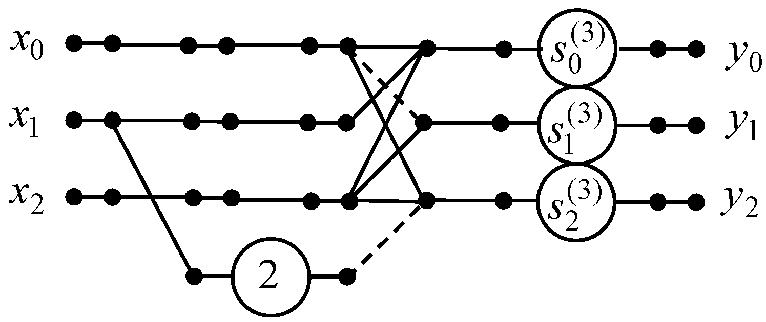
We developed the 3-point real DTT algorithm via construction of the data flow graph that is shown in Figure 1. If we apply the three-point DTT algorithm, we can reduce the number of multiplications from 8 to 3, while the number of additions remains unchanged.

3.2. Algorithm for 4-Point DTT

Let us construct the algorithm for 4-point real-valued DTT, which is expressed as

$${\mathbf{Y}}_{4\times 1}=\mathit{diag}({\mathbf{s}}_{4\times 1}){\mathbf{C}}_4{\mathbf{X}}_{4\times 1},$$

(8)

where ${\mathbf{Y}}_{4\times 1}={\left[y_0,y_1,y_2,y_3\right]}^{\mathrm{T}}$, ${\mathbf{X}}_{4\times 1}={\left[x_0,x_1,x_2,x_3\right]}^{\mathrm{T}}$, ${\mathbf{C}}_4=\left[\begin{array}{cccc}\mathbf{1}& \mathbf{1}& \mathbf{1}& \mathbf{1}\\ -\mathbf{3}& -\mathbf{1}& \mathbf{1}& \mathbf{3}\\ \mathbf{1}& -\mathbf{1}& -\mathbf{1}& \mathbf{1}\\ -\mathbf{1}& \mathbf{3}& -\mathbf{3}& \mathbf{1}\end{array}\right]$. Vector ${\mathbf{s}}_{4\times 1}={\left[s_0^{(4)},s_1^{(4)},s_2^{(4)},s_3^{(4)}\right]}^{\mathrm{T}}$ was computed using expression (5) as ${\mathbf{s}}_{4\times 1}$=${\left[{\displaystyle \frac{1}{2}},{\displaystyle \frac{1}{\sqrt{20}}},{\displaystyle \frac{1}{2}},{\displaystyle \frac{1}{\sqrt{20}}}\right]}^{\mathrm{T}}$ or ${\mathbf{s}}_{4\times 1}$≈${\left[0.5000,0.2236,0.5000,0.2236\right]}^{\mathrm{T}}$.

We use the structural approach [37,38,39,40] to design the algorithm for 4-point real DTT. Let us define the permutations ${\pi }_1=\left(\begin{array}{cccc}1& 2& 3& 4\\ 1& 3& 2& 4\end{array}\right)$ and ${\pi }_2=\left(\begin{array}{cccc}1& 2& 3& 4\\ 1& 2& 4& 3\end{array}\right)$ for altering the order of the rows and columns of matrix ${\mathbf{C}}_4$, respectively. The obtained matrix ${\mathbf{C}}_4^{(a)}$ matches the matrix pattern $\left[\begin{array}{cc}{\mathbf{A}}_2& {\mathbf{A}}_2\\ {\mathbf{B}}_2& -{\mathbf{B}}_2\end{array}\right]$ where ${\mathbf{A}}_2={\mathbf{H}}_2$, ${\mathbf{B}}_2=\left[\begin{array}{cc}-3& -1\\ -1& 3\end{array}\right]$. Therefore, ${\mathbf{C}}_4^{(a)}=({\mathbf{A}}_2\oplus {\mathbf{B}}_2)({\mathbf{H}}_2\otimes {\mathbf{I}}_2)$. The matrix ${\mathbf{B}}_2$ can be decomposed as [37,38]:

$${\mathbf{B}}_2={\mathbf{T}}_{2\times 3}^{(4)}\mathit{diag}(-2,4,-1){\mathbf{T}}_{3\times 2}^{(3)},$$

(9)

where ${\mathbf{T}}_{3\times 2}^{(3)}=\left[\begin{array}{cc}1& 0\\ 0& 1\\ 1& 1\end{array}\right],$ ${\mathbf{T}}_{2\times 3}^{(4)}=\left[\begin{array}{ccc}1& 0& 1\\ 0& 1& 1\end{array}\right]$.

We give the matrix factorization for the algorithm of 4-point DTT as follows:

$${\mathbf{Y}}_{4\times 1}=\mathit{diag}({\mathbf{s}}_{4\times 1}){\mathbf{P}}_4^{(1)}{\mathbf{W}}_{4\times 5}{\mathbf{D}}_5{\mathbf{W}}_{5\times 4}{\mathbf{W}}_4{\mathbf{P}}_4^{(0)}{\mathbf{X}}_{4\times 1},$$

(10)

where

$${\mathbf{D}}_5=\mathit{diag}\left(1,1,-2,4,-1\right);{\mathbf{W}}_{4\times 5}={\mathbf{I}}_2\oplus {\mathbf{T}}_{2\times 3}^{(4)},{\mathbf{W}}_{5\times 4}={\mathbf{H}}_2\oplus {\mathbf{T}}_{3\times 2}^{(3)},{\mathbf{W}}_4={\mathbf{H}}_2\otimes {\mathbf{I}}_2,$$

(11)

$${\mathbf{P}}_4^{(1)}=\left[\begin{array}{cccc}\mathbf{1}& & & \\ & & \mathbf{1}& \\ & \mathbf{1}& & \\ & & & \mathbf{1}\end{array}\right],{\mathbf{P}}_4^{(0)}=\left[\begin{array}{cccc}\mathbf{1}& & & \\ & \mathbf{1}& & \\ & & & \mathbf{1}\\ & & \mathbf{1}& \end{array}\right].$$

(12)

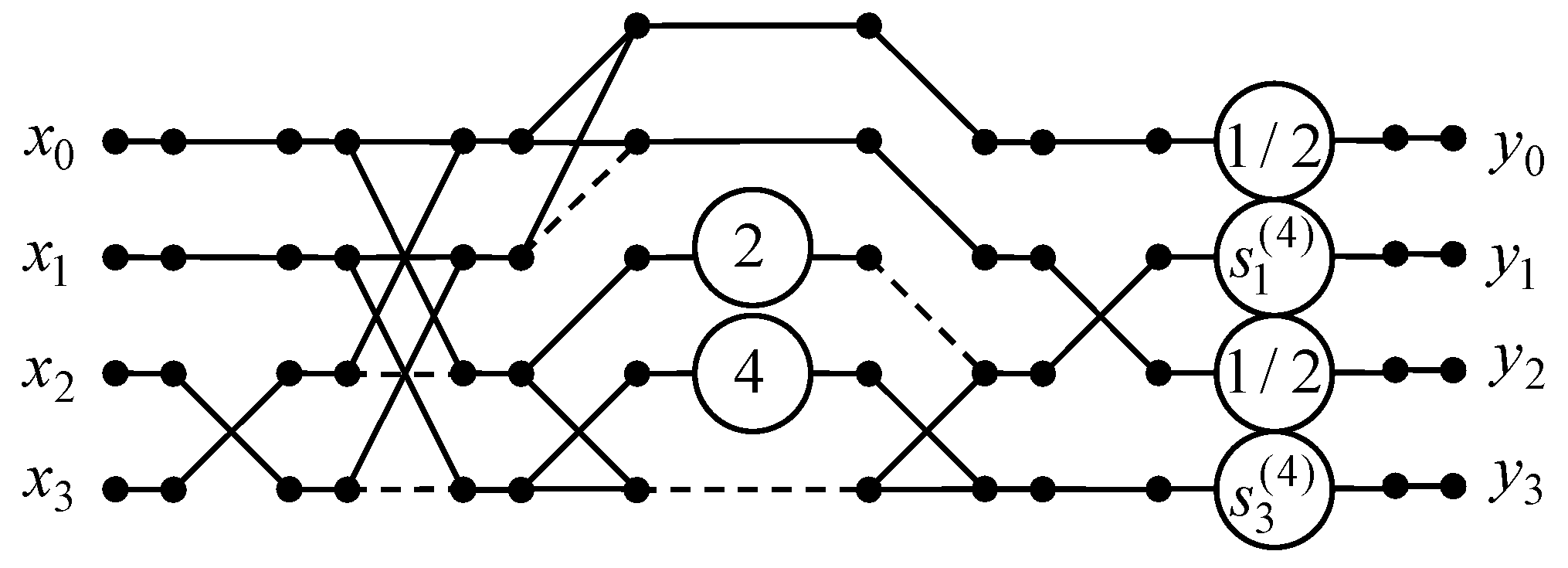
Figure 2 shows a data flow graph of the proposed four-point DTT algorithm. Note that for N = 4, the initial 4-point real DTT requires 8 real-valued multiplications, 8 shifts, and 12 additions. If we use the proposed four-point DTT algorithm, then the number of multiplications, additions, and shifts may be reduced from 8 to 2, from 12 to 9, and from 8 to 5, respectively.

3.3. Algorithm for 5-Point DTT

To develop the algorithm for 5-point 1D DTT, we express this transform as follows:

$${\mathbf{Y}}_{5\times 1}=\mathit{diag}{(\mathbf{s}}_{5\times 1}){\mathbf{C}}_5{\mathbf{X}}_{5\times 1},$$

(13)

where ${\mathbf{C}}_5=\left[\begin{array}{ccccc}\mathbf{1}& \mathbf{1}& \mathbf{1}& \mathbf{1}& \mathbf{1}\\ -\mathbf{2}& -\mathbf{1}& \mathbf{0}& \mathbf{1}& \mathbf{2}\\ \mathbf{2}& -\mathbf{1}& -\mathbf{2}& -\mathbf{1}& \mathbf{2}\\ -\mathbf{1}& \mathbf{2}& \mathbf{0}& -\mathbf{2}& \mathbf{1}\\ \mathbf{1}& -\mathbf{4}& \mathbf{6}& -\mathbf{4}& \mathbf{1}\end{array}\right]$, ${\mathbf{Y}}_{5\times 1}=\left[\begin{array}{c}{y}_0\\ y_1\\ y_2\\ y_3\\ y_4\end{array}\right]$, ${\mathbf{X}}_{5\times 1}=\left[\begin{array}{c}{x}_0\\ x_1\\ x_2\\ x_3\\ x_4\end{array}\right]$.

The vector ${\mathbf{s}}_{5\times 1}={\left[s_0^{(5)},s_1^{(5)},s_2^{(5)},s_3^{(5)},s_4^{(5)}\right]}^{\mathrm{T}}$ is computed by expression (5) where $s_1^{(5)}={\displaystyle \frac{2p_1}{\sqrt{d(1,N})}}$, $s_3^{(5)}={\displaystyle \frac{2p_3}{\sqrt{d(3,N})}}$, $s_4^{(5)}={\displaystyle \frac{p_4}{N\sqrt{d(4,N})}}$. As a result, we yield ${\mathbf{s}}_{5\times 1}$ = ${\left[{\displaystyle \frac{1}{\sqrt{5}}},{\displaystyle \frac{1}{\sqrt{10}}},{\displaystyle \frac{1}{\sqrt{14}}},{\displaystyle \frac{1}{\sqrt{10}}},{\displaystyle \frac{1}{\sqrt{70}}}\right]}^{\mathrm{T}}$ or ${\mathbf{s}}_{5\times 1}$ = ${\left[0.4472,0.3162,0.2673,0.3162,0.1195\right]}^{\mathrm{T}}$.

Denoting $a_5=1;$ $b_5$ = $2;c_5$ = $4;d_5$ = $6,$ we obtain the matrix

$${\mathbf{C}}_5^{(a)}=\left[\begin{array}{ccccc}{\mathit{a}}_5& {\mathit{a}}_5& {\mathit{a}}_5& {\mathit{a}}_5& {\mathit{a}}_5\\ -{\mathit{b}}_5& -{\mathit{a}}_5& \mathbf{0}& {\mathit{a}}_5& {\mathit{b}}_5\\ {\mathit{b}}_5& -{\mathit{a}}_5& -{\mathit{b}}_5& -{\mathit{a}}_5& {\mathit{b}}_5\\ -{\mathit{a}}_5& {\mathit{b}}_5& \mathbf{0}& -{\mathit{b}}_5& {\mathit{a}}_5\\ {\mathit{a}}_5& -{\mathit{c}}_5& {\mathit{d}}_5& -{\mathit{c}}_5& {\mathit{a}}_5\end{array}\right].$$

(14)

We again apply the structural approach [37,38,39,40] to develop the algorithm for 5-point 1D real DTT. The permutations ${\pi }_3$ and ${\pi }_4$ are defined to alter the order of columns and rows of matrix ${\mathbf{C}}_5$, respectively, as

$${\pi }_3=\left(\begin{array}{cc}1& 2\\ 1& 2\end{array}\begin{array}{ccc}3& 4& 5\\ 3& 5& 4\end{array}\right)\mathrm{and}{\pi }_4=\left(\begin{array}{cc}1& 2\\ 3& 5\end{array}\begin{array}{ccc}3& 4& 5\\ 1& 4& 2\end{array}\right).$$

(15)

After permutation, the obtained matrix ${\mathbf{C}}_5^{(b)}=\left[\begin{array}{ccccc}{\mathit{b}}_5& -{\mathit{a}}_5& -{\mathit{b}}_5& {\mathit{b}}_5& -{\mathit{a}}_5\\ {\mathit{a}}_5& -{\mathit{c}}_5& {\mathit{d}}_5& {\mathit{a}}_5& -{\mathit{c}}_5\\ {\mathit{a}}_5& {\mathit{a}}_5& {\mathit{a}}_5& {\mathit{a}}_5& {\mathit{a}}_5\\ -{\mathit{a}}_5& {\mathit{b}}_5& \mathbf{0}& {\mathit{a}}_5& -{\mathit{b}}_5\\ -{\mathit{b}}_5& -{\mathit{a}}_5& \mathbf{0}& {\mathit{b}}_5& {\mathit{a}}_5\end{array}\right]$ is decomposed into two components [37,39]:

$${\mathbf{C}}_5^{(b)}={\mathbf{C}}_5^{(c)}+{\mathbf{C}}_5^{(d)},$$

(16)

where ${\mathbf{C}}_5^{(c)}=\left[\begin{array}{ccccc}& & -{\mathit{b}}_5& & \\ & & {\mathit{d}}_5& & \\ {\mathit{a}}_5& {\mathit{a}}_5& {\mathit{a}}_5& {\mathit{a}}_5& {\mathit{a}}_5\\ & & \mathbf{0}& & \\ & & \mathbf{0}& & \end{array}\right]$ and ${\mathbf{C}}_5^{(d)}=\left[\begin{array}{ccccc}{\mathit{b}}_5& -{\mathit{a}}_5& & {\mathit{b}}_5& -{\mathit{a}}_5\\ {\mathit{a}}_5& -{\mathit{c}}_5& & {\mathit{a}}_5& -{\mathit{c}}_5\\ & & & & \\ -{\mathit{a}}_5& {\mathit{b}}_5& & {\mathit{a}}_5& -{\mathit{b}}_5\\ -{\mathit{b}}_5& -{\mathit{a}}_5& & {\mathit{b}}_5& {\mathit{a}}_5\end{array}\right]$.

The structure of matrix ${\mathbf{C}}_5^{(c)}$ allows for reducing the number of operations without further transforms because the elements in the third row are identical except for the sign. After eliminating the rows and columns having only zero elements in matrix ${\mathbf{C}}_5^{(d)}$, we yield matrix ${\mathbf{C}}_4^{(d)}$:

$${\mathbf{C}}_4^{(d)}=\left[\begin{array}{cccc}{\mathit{b}}_5& -{\mathit{a}}_5& {\mathit{b}}_5& -{\mathit{a}}_5\\ {\mathit{a}}_5& -{\mathit{c}}_5& {\mathit{a}}_5& -{\mathit{c}}_5\\ -{\mathit{a}}_5& {\mathit{b}}_5& {\mathit{a}}_5& -{\mathit{b}}_5\\ -{\mathit{b}}_5& -{\mathit{a}}_5& {\mathit{b}}_5& {\mathit{a}}_5\end{array}\right].$$

(17)

Matrix ${\mathbf{C}}_4^{(d)}$ matches the template $\left[\begin{array}{cc}{\mathbf{A}}_2^{(0)}& {\mathbf{A}}_2^{(0)}\\ {\mathbf{B}}_2^{(0)}& {-\mathbf{B}}_2^{(0)}\end{array}\right]$, where ${\mathbf{A}}_2^{(0)}=\left[\begin{array}{cc}{b}_5& -a_5\\ a_5& -c_5\end{array}\right]$ and ${\mathbf{B}}_2^{(0)}=\left[\begin{array}{cc}-a_5& b_5\\ -b_5& -a_5\end{array}\right]$. Hence, matrix ${\mathbf{C}}_4^{(d)}$ can be factorized as [37,38]:

$${\mathbf{C}}_4^{(d)}=({\mathbf{A}}_2^{(0)}\oplus {\mathbf{B}}_2^{(0)})({\mathbf{H}}_2\otimes {\mathbf{I}}_2).$$

(18)

Let us swap the rows of matrix ${\mathbf{A}}_2^{(0)}$ and alter the sign of the second row of matrix ${\mathbf{B}}_2^{(0)}$. Then, the obtained matrices ${\mathbf{A}}_2^{(1)}=\left[\begin{array}{cc}{a}_5& -c_5\\ b_5& -a_5\end{array}\right]$ and ${\mathbf{B}}_2^{(1)}=\left[\begin{array}{cc}-a_5& b_5\\ b_5& a_5\end{array}\right]$ match the templates $\left[\begin{array}{cc}a& b\\ c& -a\end{array}\right]$ and $\left[\begin{array}{cc}e& d\\ d& -e\end{array}\right]$, where $a{=a}_5;b=-c_5;c{=b}_5;d{=b}_5;e=-a_5$. Then [37,40],

$${\mathbf{C}}_4^{(d)}={\mathbf{P}}_4({\mathbf{T}}_{2\times 3}^{(3)}\oplus {\mathbf{T}}_{2\times 3}^{(4)})\mathit{diag}(b_5-a_5,-c_5+a_5,-a_5,-a_5-b_5,a_5-b_5,b_5)({\mathbf{T}}_{3\times 2}^{(4)}\oplus {\mathbf{T}}_{3\times 2}^{(3)})({\mathbf{H}}_2\otimes {\mathbf{I}}_2),$$

(19)

where ${\mathbf{P}}_4=\left[\begin{array}{cccc}& \mathbf{1}& & \\ \mathbf{1}& & & \\ & & \mathbf{1}& \\ & & & -\mathbf{1}\end{array}\right]$, ${\mathbf{T}}_{2\times 3}^{(3)}=\left[\begin{array}{ccc}\mathbf{0}& \mathbf{1}& \mathbf{1}\\ \mathbf{1}& \mathbf{0}& \mathbf{1}\end{array}\right]$, ${\mathbf{T}}_{3\times 2}^{(4)}=\left[\begin{array}{cc}\mathbf{1}& \mathbf{0}\\ \mathbf{0}& \mathbf{1}\\ -\mathbf{1}& \mathbf{1}\end{array}\right]$. Matrices ${\mathbf{T}}_{2\times 3}^{(4)}$ and ${\mathbf{T}}_{3\times 2}^{(3)}$ are defined as in expression (9).

Based on Equations (16) and (19), we derive the factorization of the 5-point DTT matrix:

$${\mathbf{Y}}_{5\times 1}=\mathit{diag}{(\mathbf{s}}_{5\times 1}){\mathbf{P}}_5^{(1)}{\mathbf{W}}_{5\times 6}{\mathbf{W}}_6^{(1)}{\mathbf{W}}_{6\times 8}{\mathbf{D}}_8{\mathbf{W}}_{8\times 6}{\mathbf{W}}_6^{(0)}{\mathbf{W}}_{6\times 5}{\mathbf{P}}_5^{(0)}{\mathbf{X}}_{5\times 1},$$

(20)

where

$${\mathbf{W}}_{6\times 8}={\mathbf{T}}_{2\times 3}^{(3)}\oplus {\mathbf{I}}_2\oplus {\mathbf{T}}_{2\times 3}^{(4)},{\mathbf{W}}_{8\times 6}={\mathbf{T}}_{3\times 2}^{(4)}\oplus {\mathbf{I}}_2\oplus {\mathbf{T}}_{3\times 2}^{(3)},{\mathbf{D}}_8=\mathit{diag}(1,-3,-1,2,1,-3,-1,2),$$

(21)

$${\mathbf{P}}_5^{(0)}=\left[\begin{array}{ccccc}\mathbf{1}& & & & \\ & \mathbf{1}& & & \\ & & \mathbf{1}& & \\ & & & & \mathbf{1}\\ & & & \mathbf{1}& \end{array}\right],{\mathbf{P}}_5^{(1)}=\left[\begin{array}{ccccc}& & \mathbf{1}& & \\ & & & & \mathbf{1}\\ \mathbf{1}& & & & \\ & & & \mathbf{1}& \\ & \mathbf{1}& & & \end{array}\right],$$

(22)

$${\mathbf{W}}_6^{(0)}=\left[\begin{array}{cccccc}\mathbf{1}& & & & \mathbf{1}& \\ & \mathbf{1}& & & & \mathbf{1}\\ & & \mathbf{1}& & & \\ & & & \mathbf{1}& & \\ \mathbf{1}& & & & -\mathbf{1}& \\ & \mathbf{1}& & & & -\mathbf{1}\end{array}\right],{\mathbf{W}}_6^{(1)}=\left[\begin{array}{cccccc}& \mathbf{1}& & & & \\ \mathbf{1}& & & & & \\ & & \mathbf{1}& & & \\ & & & \mathbf{1}& & \\ & & & & \mathbf{1}& \\ & & & & & -\mathbf{1}\end{array}\right],$$

(23)

$${\mathbf{W}}_{6\times 5}=\left[\begin{array}{ccccc}\mathbf{1}& & & & \\ & \mathbf{1}& & & \\ & & \mathbf{1}& & \\ \mathbf{1}& \mathbf{1}& & \mathbf{1}& \mathbf{1}\\ & & & \mathbf{1}& \\ & & & & \mathbf{1}\end{array}\right],{\mathbf{W}}_{5\times 6}=\left[\begin{array}{cccccc}\mathbf{1}& & -\mathbf{1}& & & \\ & \mathbf{1}& \mathbf{3}& & & \\ & & \mathbf{1}/\mathbf{2}& \mathbf{1}& & \\ & & & & \mathbf{1}& \\ & & & & & \mathbf{1}\end{array}\right].$$

(24)

As was mentioned in Section 2, an empty cell in matrices means it contains zero.

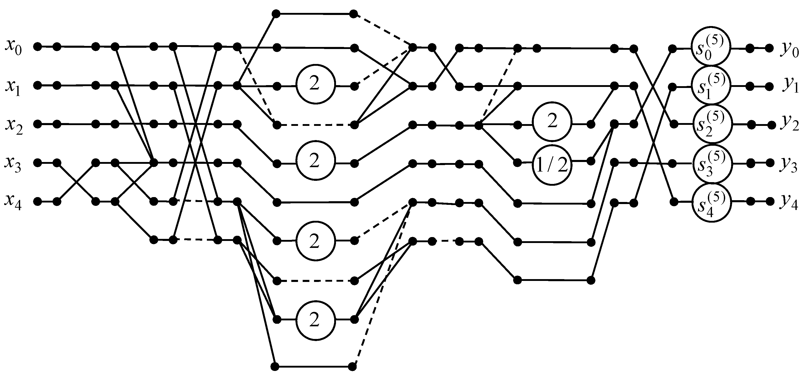
A data flow graph of the developed 5-point DTT algorithm is presented in Figure 3. Note that the original 5-point real DTT requires 23 real-valued multiplications and 18 additions, as two entries in the transform matrix are equal to zero. Using the proposed 5-point DTT algorithm, the required number of multiplications can be reduced from 23 to 5. The number of additions is increased from 18 to 19, and 6 shifts are required.

3.4. Algorithm for 6-Point DTT

Let us obtain the algorithm for 6-point 1D DTT, which is expressed as follows:

$${\mathbf{Y}}_{6\times 1}=\mathit{diag}({\mathbf{s}}_{6\times 1}){\mathbf{C}}_6{\mathbf{X}}_{6\times 1},$$

(25)

where ${\mathbf{C}}_6=\left[\begin{array}{cccccc}\mathbf{1}& \mathbf{1}& \mathbf{1}& \mathbf{1}& \mathbf{1}& \mathbf{1}\\ -\mathbf{5}& -\mathbf{3}& -\mathbf{1}& \mathbf{1}& \mathbf{3}& \mathbf{5}\\ \mathbf{5}& -\mathbf{1}& -\mathbf{4}& -\mathbf{4}& -\mathbf{1}& \mathbf{5}\\ -\mathbf{5}& \mathbf{7}& \mathbf{4}& -\mathbf{4}& -\mathbf{7}& \mathbf{5}\\ \mathbf{1}& -\mathbf{3}& \mathbf{2}& \mathbf{2}& -\mathbf{3}& \mathbf{1}\\ -\mathbf{1}& \mathbf{5}& -\mathbf{10}& \mathbf{10}& -\mathbf{5}& \mathbf{1}\end{array}\right]$, ${\mathbf{Y}}_{6\times 1}=\left[\begin{array}{c}{y}_0\\ y_1\\ y_2\\ y_3\\ y_4\\ y_5\end{array}\right]$, ${\mathbf{X}}_{6\times 1}=\left[\begin{array}{c}{x}_0\\ x_1\\ x_2\\ x_3\\ x_4\\ x_5\end{array}\right]$.

The vector ${\mathbf{s}}_{6\times 1}={\left[s_0^{(6)},s_1^{(6)},s_2^{(6)},s_3^{(6)},s_4^{(6)},s_5^{(6)}\right]}^{\mathrm{T}}$ is computed by expression (5), where $s_2^{(6)}={\displaystyle \frac{2p_2}{3\sqrt{d(2,N})}}$, $s_3^{(6)}={\displaystyle \frac{2p_3}{3\sqrt{d(3,N})}}$. As a result, we yield ${\mathbf{s}}_{6\times 1}$=${\left[{\displaystyle \frac{1}{\sqrt{6}}},{\displaystyle \frac{1}{\sqrt{70}}},{\displaystyle \frac{1}{2\sqrt{21}}},{\displaystyle \frac{1}{2\sqrt{45}}},{\displaystyle \frac{1}{\sqrt{28}}},{\displaystyle \frac{1}{\sqrt{252}}}\right]}^{\mathrm{T}}$ or ${\mathbf{s}}_{6\times 1}$≈${\left[0.4082,0.1195,0.1091,0.0745,0.1890,0.0630\right]}^{\mathrm{T}}$.

Let us denote $a_6=1;$ $b_6=2;c_6=3;d_6$ = $4;e_6$ = $5$; $f_6=7;$ $g_6=10;$ then, matrix ${\mathbf{C}}_6$ is represented as

$${\mathbf{C}}_6^{(a)}=\left[\begin{array}{cccccc}{\mathit{a}}_6& {\mathit{a}}_6& {\mathit{a}}_6& {\mathit{a}}_6& {\mathit{a}}_6& {\mathit{a}}_6\\ -{\mathit{e}}_6& -{\mathit{c}}_6& -{\mathit{a}}_6& {\mathit{a}}_6& {\mathit{c}}_6& {\mathit{e}}_6\\ {\mathit{e}}_6& -{\mathit{a}}_6& -{\mathit{d}}_6& -{\mathit{d}}_6& -{\mathit{a}}_6& {\mathit{e}}_6\\ -{\mathit{e}}_6& {\mathit{f}}_6& {\mathit{d}}_6& -{\mathit{d}}_6& -{\mathit{f}}_6& {\mathit{e}}_6\\ {\mathit{a}}_6& -{\mathit{c}}_6& {\mathit{b}}_6& {\mathit{b}}_6& -{\mathit{c}}_6& {\mathit{a}}_6\\ -{\mathit{a}}_6& {\mathit{e}}_6& -{\mathit{g}}_6& {\mathit{g}}_6& -{\mathit{e}}_6& {\mathit{a}}_6\end{array}\right].$$

(26)

The columns and rows of ${\mathbf{C}}_6$ are permutated according to ${\pi }_5$ and ${\pi }_6$, which are defined in the following form: ${\pi }_5=\left(\begin{array}{cc}1& 2\\ 1& 6\end{array}\begin{array}{cccc}3& 4& 5& 6\\ 3& 4& 2& 5\end{array}\right)$ and ${\pi }_6=\left(\begin{array}{cc}1& 2\\ 2& 4\end{array}\begin{array}{cccc}3& 4& 5& 6\\ 1& 6& 3& 5\end{array}\right)$. The permutation matrices are as follows:

$${\mathbf{P}}_6^{(1)}=\left[\begin{array}{cccccc}& & \mathbf{1}& & & \\ \mathbf{1}& & & & & \\ & & & & \mathbf{1}& \\ & \mathbf{1}& & & & \\ & & & & & \mathbf{1}\\ & & & \mathbf{1}& & \end{array}\right],{\mathbf{P}}_6^{(0)}=\left[\begin{array}{cccccc}\mathbf{1}& & & & & \\ & & & & & \mathbf{1}\\ & & \mathbf{1}& & & \\ & & & \mathbf{1}& & \\ & \mathbf{1}& & & & \\ & & & & \mathbf{1}& \end{array}\right].$$

(27)

The resulting matrix

$${\mathbf{C}}_6^{(b)}=\left[\begin{array}{cccccc}-{\mathit{e}}_6& {\mathit{e}}_6& -{\mathit{a}}_6& {\mathit{a}}_6& -{\mathit{c}}_6& {\mathit{c}}_6\\ -{\mathit{e}}_6& {\mathit{e}}_6& {\mathit{d}}_6& -{\mathit{d}}_6& {\mathit{f}}_6& -{\mathit{f}}_6\\ {\mathit{a}}_6& {\mathit{a}}_6& {\mathit{a}}_6& {\mathit{a}}_6& {\mathit{a}}_6& {\mathit{a}}_6\\ -{\mathit{a}}_6& {\mathit{a}}_6& -{\mathit{g}}_6& {\mathit{g}}_6& {\mathit{e}}_6& -{\mathit{e}}_6\\ {\mathit{e}}_6& {\mathit{e}}_6& -{\mathit{d}}_6& -{\mathit{d}}_6& -{\mathit{a}}_6& -{\mathit{a}}_6\\ {\mathit{a}}_6& {\mathit{a}}_6& {\mathit{b}}_6& {\mathit{b}}_6& -{\mathit{c}}_6& -{\mathit{c}}_6\end{array}\right]$$

(28)

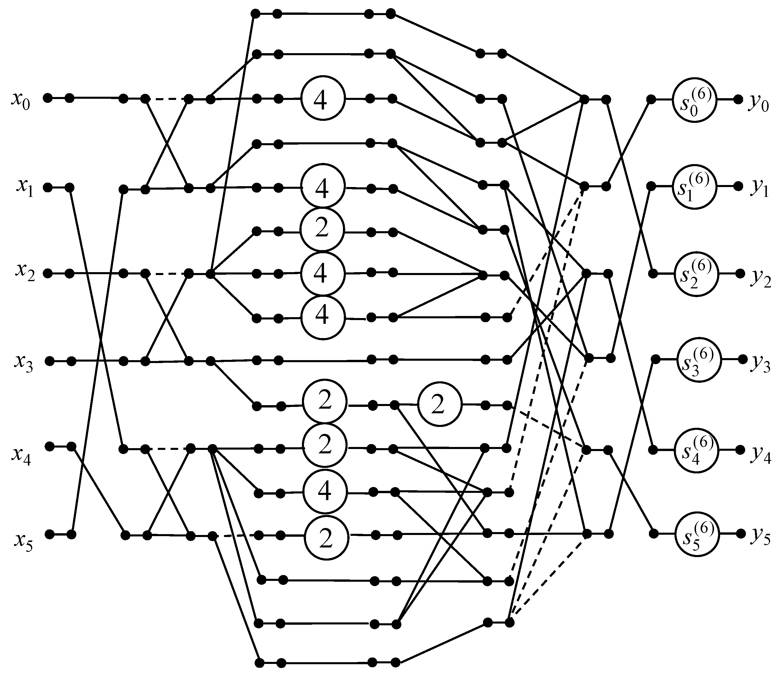
contains repeated elements that enable butterfly module extraction and construction of the data flow graph for 6-point 1D DTT calculation. A derived data flow graph of the proposed 6-point 1D DTT algorithm is shown in Figure 4.

Further, we compose the factorization of the matrix of 6-point 1D DTT from the matrices for calculations at each layer of the graph. Thus, at the first layer, we obtain the matrix ${\mathbf{W}}_6={\mathbf{W}}_2\oplus {\mathbf{W}}_2\oplus {\mathbf{W}}_2,$ where ${\mathbf{W}}_2=\left[\begin{array}{cc}-1& 1\\ 1& 1\end{array}\right]$.

The second layer of calculations is described by matrix ${\mathbf{W}}_{16\times 6}$ which can be expressed via matrix ${({\mathbf{W}}_{16\times 6})}^{\mathrm{T}}$ as follows:

$${({\mathbf{W}}_{16\times 6})}^{\mathrm{T}}=\left[\begin{array}{cccccccccccccccc}& 1& 1& & & & & & & & & & & & & \\ & & & 1& 1& & & & & & & & & & & \\ 1& & & & & 1& 1& 1& & & & & & & & \\ & & & & & & & & 1& 1& & & & & & \\ & & & & & & & & & & 1& 1& & 1& 1& \\ & & & & & & & & & & & & -1& & & 1\end{array}\right].$$

(29)

In this matrix and the matrices below, an empty cell indicates that it contains zero. We have diagonal matrix ${\mathbf{D}}_{16}=\mathit{diag}(1,1,4,1,4,2,4,4,1,2,2,4,2,1,1,1)$ at the third layer of calculation and matrices ${\mathbf{W}}_{14\times 16}$ and ${\mathbf{W}}_{6\times 14}$ at the fourth and fifth layers of calculation:

$${\mathbf{W}}_{14\times 16}=\left[\begin{array}{cccccccccccccccc}1& & & & & & & & & & & & & & & \\ & 1& & & & & & & & & & & & & & \\ & 1& 1& & & & & & & & & & & & & \\ & & & 1& & & & & & & & & & & & \\ & & & 1& 1& & & & & & & & & & & \\ & & & & & 1& 1& 1& & & & & & & & \\ & & & & & & & 1& & & & & & & & \\ & & & & & & & & 1& & & & & & & \\ & & & & & & & & & 2& & & & & & \\ & & & & & & & & & & 1& & & & 1& \\ & & & & & & & & & & 1& 1& & & 1& \\ & & & & & & & & & 1& & & 1& & & \\ & & & & & & & & & & & 1& & 1& & \\ & & & & & & & & & & & & & & & 1\end{array}\right],$$

(30)

$${\mathbf{W}}_{6\times 14}=\left[\begin{array}{cccccccccccccc}1& & 1& & & & & & & 1& & & & \\ & & 1& & & & -1& & & & -1& & & \\ & & & 1& & & & 1& & & & & & 1\\ & 1& & & & 1& & & & & & & -1& \\ & & & & 1& & & & -1& & & & & -1\\ & & & 1& & & & & & & & 1& & -1\end{array}\right].$$

(31)

Next, we take into consideration the permutation matrices ${\mathbf{P}}_6^{(1)}$ and ${\mathbf{P}}_6^{(0)}$ and matrices ${\mathbf{W}}_6$, ${\mathbf{W}}_{16\times 6}$, ${\mathbf{W}}_{14\times 16}$, ${\mathbf{W}}_{6\times 14}$ at different computing layers of the data flow graph from Figure 4 to obtain factorization of the 6-point 1D DTT matrix:

$${\mathbf{Y}}_{6\times 1}=\mathit{diag}({\mathbf{s}}_{6\times 1}){\mathbf{P}}_6^{(1)}{\mathbf{W}}_{6\times 14}{\mathbf{W}}_{14\times 16}{\mathbf{D}}_{16}{\mathbf{W}}_{16\times 6}{\mathbf{W}}_6{\mathbf{P}}_6^{(0)}{\mathbf{X}}_{6\times 1}.$$

(32)

Let us consider the data flow graph of the developed 6-point 1D DTT algorithm (Figure 4). It should be noted that the initial 6-point real DTT requires 36 real-valued multiplications and 30 additions. If we apply the developed 6-point 1D DTT algorithm, the number of real-valued multiplications is reduced to 6. The number of additions is decreased from 30 to 27, and 15 shifts are required.

3.5. Algorithm for 7-Point DTT

To design the algorithm for the 7-point 1D DTT we represent this transform as follows:

$${\mathbf{Y}}_{7\times 1}=\mathit{diag}({\mathbf{s}}_{7\times 1}){\mathbf{C}}_7{\mathbf{X}}_{7\times 1},$$

(33)

where ${\mathbf{C}}_7=\left[\begin{array}{ccccccc}\mathbf{1}& \mathbf{1}& \mathbf{1}& \mathbf{1}& \mathbf{1}& \mathbf{1}& \mathbf{1}\\ -\mathbf{3}& -\mathbf{2}& -\mathbf{1}& \mathbf{0}& \mathbf{1}& \mathbf{2}& \mathbf{3}\\ \mathbf{5}& \mathbf{0}& -\mathbf{3}& -\mathbf{4}& -\mathbf{3}& \mathbf{0}& \mathbf{5}\\ -\mathbf{1}& \mathbf{1}& \mathbf{1}& \mathbf{0}& -\mathbf{1}& -\mathbf{1}& \mathbf{1}\\ \mathbf{3}& -\mathbf{7}& \mathbf{1}& \mathbf{6}& \mathbf{1}& -\mathbf{7}& \mathbf{3}\\ -\mathbf{1}& \mathbf{4}& -\mathbf{5}& \mathbf{0}& \mathbf{5}& -\mathbf{4}& \mathbf{1}\\ \mathbf{1}& -\mathbf{6}& \mathbf{15}& -\mathbf{20}& \mathbf{15}& -\mathbf{6}& \mathbf{1}\end{array}\right]$, ${\mathbf{Y}}_{7\times 1}=\left[\begin{array}{c}{y}_0\\ y_1\\ y_2\\ y_3\\ y_4\\ y_5\\ y_6\end{array}\right]$, ${\mathbf{X}}_{7\times 1}=\left[\begin{array}{c}{x}_0\\ x_1\\ x_2\\ x_3\\ x_4\\ x_5\\ x_6\end{array}\right]$.

Vector ${\mathbf{s}}_{7\times 1}={\left[s_0^{(7)},s_1^{(7)},s_2^{(7)},s_3^{(7)},s_4^{(7)},s_5^{(7)},s_6^{(7)}\right]}^{\mathrm{T}}$ is computed by expression (5), where $s_1^{(7)}={\displaystyle \frac{2p_1}{\sqrt{d(1,N})}}$, $s_3^{(7)}={\displaystyle \frac{5p_3}{\sqrt{d(3,N})}}$, $s_5^{(7)}={\displaystyle \frac{3p_5}{\sqrt{d(5,N})}}$, $s_6^{(7)}={\displaystyle \frac{p_6}{N\sqrt{d(6,N})}}$. As a result, we yield ${\mathbf{s}}_{7\times 1}$ = [${\displaystyle \frac{1}{\sqrt{7}}}$, ${\displaystyle \frac{1}{\sqrt{28}}}$, ${\displaystyle \frac{1}{2\sqrt{21}}}$, ${\displaystyle \frac{1}{\sqrt{6}}}$, ${\displaystyle \frac{1}{\sqrt{154}}}$, ${\displaystyle \frac{1}{2\sqrt{21}}}$, ${\displaystyle \frac{1}{\sqrt{924}}}{]}^{\mathrm{T}}$ or ${\mathbf{s}}_{7\times 1}$ ≈ [0.3780, 0.1890, 0.1091, 0.4082, 0.0806, 0.1091, 0.0329${]}^{\mathrm{T}}$.

If we denote $a_7=1;b_7=2;c_7=3;d_7=4;e_7=5;f_7=6;g_7=7;h_7=15;k_7=20;$ matrix ${\mathbf{C}}_7$ can be represented as

$${\mathbf{C}}_7=\left[\begin{array}{ccccccc}{\mathit{a}}_7& {\mathit{a}}_7& {\mathit{a}}_7& {\mathit{a}}_7& {\mathit{a}}_7& {\mathit{a}}_7& {\mathit{a}}_7\\ -{\mathit{c}}_7& -{\mathit{b}}_7& -{\mathit{a}}_7& \mathbf{0}& {\mathit{a}}_7& {\mathit{b}}_7& {\mathit{c}}_7\\ {\mathit{e}}_7& \mathbf{0}& -{\mathit{c}}_7& -{\mathit{d}}_7& -{\mathit{c}}_7& \mathbf{0}& {\mathit{e}}_7\\ -{\mathit{a}}_7& {\mathit{a}}_7& {\mathit{a}}_7& \mathbf{0}& -{\mathit{a}}_7& -{\mathit{a}}_7& {\mathit{a}}_7\\ {\mathit{c}}_7& -{\mathit{g}}_7& {\mathit{a}}_7& {\mathit{f}}_7& {\mathit{a}}_7& -{\mathit{g}}_7& {\mathit{c}}_7\\ -{\mathit{a}}_7& {\mathit{d}}_7& -{\mathit{e}}_7& \mathbf{0}& {\mathit{e}}_7& -{\mathit{d}}_7& {\mathit{a}}_7\\ {\mathit{a}}_7& -{\mathit{f}}_7& {\mathit{h}}_7& -{\mathit{k}}_7& {\mathit{h}}_7& -{\mathit{f}}_7& {\mathit{a}}_7\end{array}\right].$$

(34)

We developed the 7-point real DTT algorithm using a sparse matrix factorization [8,28,29,41] and the structural approach [37,40]. The structural approach was used to decompose the initial DTT matrix into submatrices. Sparse matrix factorization allows for the design of the data flow graph of the algorithm. To change the order of columns and rows, we define permutations ${\pi }_7$ and ${\pi }_8$ as follows:

$${\pi }_7=\left(\begin{array}{cc}1& 2\\ 1& 7\end{array}\begin{array}{ccccc}3& 4& 5& 6& 7\\ 2& 4& 6& 3& 5\end{array}\right),{\pi }_8=\left(\begin{array}{cc}1& 2\\ 2& 4\end{array}\begin{array}{ccccc}3& 4& 5& 6& 7\\ 6& 1& 3& 5& 7\end{array}\right).$$

(35)

The permutation matrices are expressed as:

$${\mathbf{P}}_7^{(1)}=\left[\begin{array}{ccccccc}& & & 1& & & \\ 1& & & & & & \\ & & & & 1& & \\ & 1& & & & & \\ & & & & & 1& \\ & & 1& & & & \\ & & & & & & 1\end{array}\right];{\mathbf{P}}_7^{(0)}=\left[\begin{array}{ccccccc}1& & & & & & \\ & & & & & & 1\\ & 1& & & & & \\ & & & 1& & & \\ & & & & & 1& \\ & & 1& & & & \\ & & & & 1& & \end{array}\right].$$

(36)

After permutation, matrix ${\mathbf{C}}_7$ acquires the following structure:

$${\mathbf{C}}_7^{(a)}=\left[\begin{array}{ccccccc}-{\mathit{c}}_7& {\mathit{c}}_7& -{\mathit{b}}_7& \mathbf{0}& {\mathit{b}}_7& -{\mathit{a}}_7& {\mathit{a}}_7\\ -{\mathit{a}}_7& {\mathit{a}}_7& {\mathit{a}}_7& \mathbf{0}& -{\mathit{a}}_7& {\mathit{a}}_7& -{\mathit{a}}_7\\ -{\mathit{a}}_7& {\mathit{a}}_7& {\mathit{d}}_7& \mathbf{0}& -{\mathit{d}}_7& -{\mathit{e}}_7& {\mathit{e}}_7\\ {\mathit{a}}_7& {\mathit{a}}_7& {\mathit{a}}_7& {\mathit{a}}_7& {\mathit{a}}_7& {\mathit{a}}_7& {\mathit{a}}_7\\ {\mathit{e}}_7& {\mathit{e}}_7& \mathbf{0}& -{\mathit{d}}_7& \mathbf{0}& -{\mathit{c}}_7& -{\mathit{c}}_7\\ {\mathit{c}}_7& {\mathit{c}}_7& -{\mathit{g}}_7& {\mathit{f}}_7& -{\mathit{g}}_7& {\mathit{a}}_7& {\mathit{a}}_7\\ {\mathit{a}}_7& {\mathit{a}}_7& -{\mathit{f}}_7& -{\mathit{k}}_7& -{\mathit{f}}_7& {\mathit{h}}_7& {\mathit{h}}_7\end{array}\right].$$

(37)

Next, matrix ${\mathbf{C}}_7^{(a)}$ is decomposed into two components:

$${\mathbf{C}}_7^{(a)}={\mathbf{C}}_7^{(b)}+{\mathbf{C}}_7^{(c)},$$

(38)

where

$${\mathbf{C}}_7^{(b)}=\left[\begin{array}{ccccccc}& & & & & & \\ & & & & & & \\ & & & & & & \\ {\mathit{a}}_7& {\mathit{a}}_7& {\mathit{a}}_7& {\mathit{a}}_7& {\mathit{a}}_7& {\mathit{a}}_7& {\mathit{a}}_7\\ & & & -{\mathit{d}}_7& & & \\ & & & {\mathit{f}}_7& & & \\ & & & -{\mathit{k}}_7& & & \end{array}\right],{\mathbf{C}}_7^{(c)}=\left[\begin{array}{ccccccc}-{\mathit{c}}_7& {\mathit{c}}_7& -{\mathit{b}}_7& & {\mathit{b}}_7& -{\mathit{a}}_7& {\mathit{a}}_7\\ -{\mathit{a}}_7& {\mathit{a}}_7& {\mathit{a}}_7& & -{\mathit{a}}_7& {\mathit{a}}_7& -{\mathit{a}}_7\\ -{\mathit{a}}_7& {\mathit{a}}_7& {\mathit{d}}_7& & -{\mathit{d}}_7& -{\mathit{e}}_7& {\mathit{e}}_7\\ & & & & & & \\ {\mathit{e}}_7& {\mathit{e}}_7& & & & -{\mathit{c}}_7& -{\mathit{c}}_7\\ {\mathit{c}}_7& {\mathit{c}}_7& -{\mathit{g}}_7& & -{\mathit{g}}_7& {\mathit{a}}_7& {\mathit{a}}_7\\ {\mathit{a}}_7& {\mathit{a}}_7& -{\mathit{f}}_7& & -{\mathit{f}}_7& {\mathit{h}}_7& {\mathit{h}}_7\end{array}\right].$$

(39)

Matrix ${\mathbf{C}}_7^{(b)}$ has identical entries in its fourth row. This allows us to reduce the number of operations without further transformations. Next, we eliminate the row and column containing only zero entries in matrix ${\mathbf{C}}_7^{(c)}$ and obtain matrix ${\mathbf{C}}_6^{(d)}$:

$${\mathbf{C}}_6^{(d)}=\left[\begin{array}{cccccc}-{\mathit{c}}_7& {\mathit{c}}_7& -{\mathit{b}}_7& {\mathit{b}}_7& -{\mathit{a}}_7& {\mathit{a}}_7\\ -{\mathit{a}}_7& {\mathit{a}}_7& {\mathit{a}}_7& -{\mathit{a}}_7& {\mathit{a}}_7& -{\mathit{a}}_7\\ -{\mathit{a}}_7& {\mathit{a}}_7& {\mathit{d}}_7& -{\mathit{d}}_7& -{\mathit{e}}_7& {\mathit{e}}_7\\ {\mathit{e}}_7& {\mathit{e}}_7& \mathbf{0}& \mathbf{0}& -{\mathit{c}}_7& -{\mathit{c}}_7\\ {\mathit{c}}_7& {\mathit{c}}_7& -{\mathit{g}}_7& -{\mathit{g}}_7& {\mathit{a}}_7& {\mathit{a}}_7\\ {\mathit{a}}_7& {\mathit{a}}_7& -{\mathit{f}}_7& -{\mathit{f}}_7& {\mathit{h}}_7& {\mathit{h}}_7\end{array}\right].$$

(40)

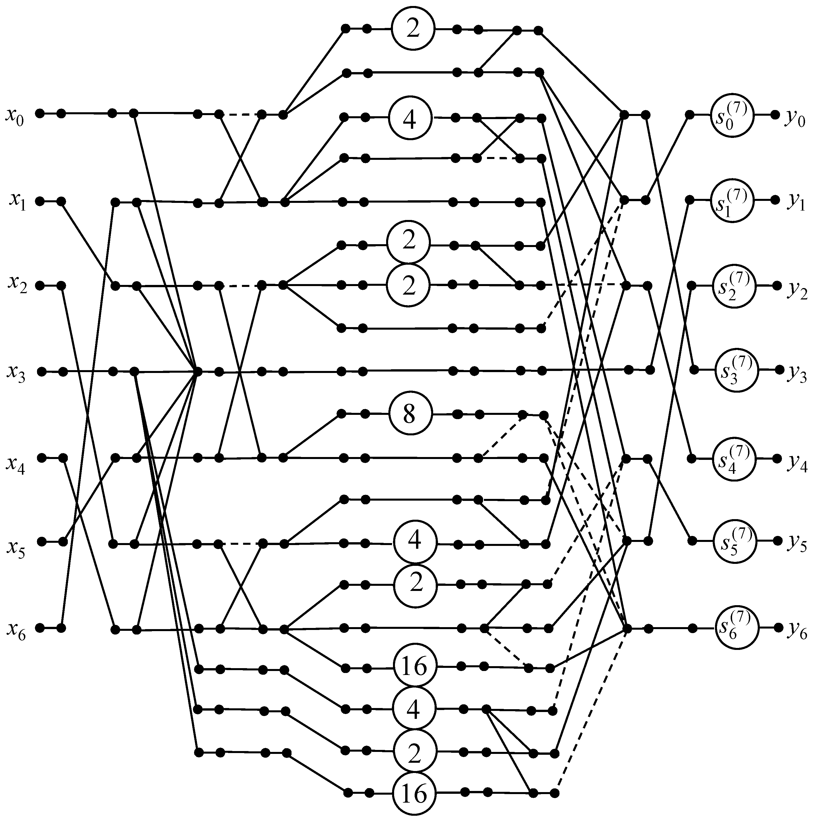
Matrix ${\mathbf{C}}_6^{(d)}$ contains repeated elements, enabling the design of the data flow graph for the 7-point 1D DTT calculation. Figure 5 shows the obtained data flow graph of the developed 7-point 1D DTT algorithm.

Further, we create the factorization of the matrix of 7-point 1D DTT using the matrices for calculations at each layer of the graph. As a result, we obtain matrix ${\mathbf{W}}_{10\times 7}$ at the first layer of calculations:

$${\mathbf{W}}_{10\times 7}=\left[\begin{array}{ccccccc}\mathbf{1}& & & & & & \\ & \mathbf{1}& & & & & \\ & & \mathbf{1}& & & & \\ \mathbf{1}& \mathbf{1}& \mathbf{1}& \mathbf{1}& \mathbf{1}& \mathbf{1}& \mathbf{1}\\ & & & & \mathbf{1}& & \\ & & & & & \mathbf{1}& \\ & & & & & & \mathbf{1}\\ & & & \mathbf{1}& & & \\ & & & \mathbf{1}& & & \\ & & & \mathbf{1}& & & \end{array}\right].$$

(41)

The second layer of calculations is described by matrix ${\mathbf{W}}_{10}$ which can be expressed as follows: ${\mathbf{W}}_{10}={\mathbf{W}}_2\oplus {\mathbf{W}}_3\oplus {\mathbf{W}}_2\oplus {\mathbf{I}}_3,$ where ${\mathbf{W}}_3=\left[\begin{array}{ccc}-1& & 1\\ & 1& \\ 1& & 1\end{array}\right]$. Matrices ${\mathbf{W}}_{19\times 10}$ and ${\mathbf{W}}_{19}$ provide calculations at the third and fifth layers of the data flow graph in Figure 5:

$${\mathbf{W}}_{19\times 10}={\mathbf{1}}_{2\times 1}\oplus {\mathbf{1}}_{3\times 1}\oplus {\mathbf{1}}_{3\times 1}\oplus 1\oplus {\mathbf{1}}_{2\times 1}\oplus {\mathbf{1}}_{2\times 1}\oplus {\mathbf{1}}_{3\times 1}\oplus {\mathbf{I}}_3,$$

(42)

$${\mathbf{W}}_{19}=\left[\begin{array}{cc}1& 1\\ & 1\end{array}\right]\oplus {\mathbf{H}}_2\oplus 1\oplus \left[\begin{array}{cc}1& \\ 1& 1\end{array}\right]\oplus {\mathbf{I}}_2\oplus \left[\begin{array}{cc}1& -1\\ & 1\end{array}\right]\oplus \left[\begin{array}{cc}1& \\ 1& 1\end{array}\right]\oplus \left[\begin{array}{ccc}1& 1& \\ & 1& \\ & -1& 1\end{array}\right]\oplus \left[\begin{array}{ccc}1& & \\ 1& 1& \\ 1& & 1\end{array}\right].$$

(43)

We have diagonal matrix

$${\mathbf{D}}_{19}=\mathit{diag}(2,1,4,1,1,2,2,1,1,8,1,1,4,2,1,1,16,4,2,16)$$

(44)

at the fourth layer of calculation, and matrix ${\mathbf{W}}_{7\times 19}$ at the sixth layer of calculation as follows:

$${\mathbf{W}}_{7\times 19}==\left[\begin{array}{ccccccccccccccccccc}1& & & & & 1& & & & & & 1& & & & & & & \\ & 1& & & & & & -1& & & & -1& & & & & & & \\ & 1& & & & & -1& & & & & & 1& & & & & & \\ & & & & & & & & 1& & & & & & & & & & \\ & & 1& & & & & & & & & & & -1& & & -1& & \\ & & & 1& & & & & & -1& & & & & 1& & & 1& \\ & & & & 1& & & & & -1& 1& & & & & 1& & & -1\end{array}\right].$$

(45)

Combining the permutation matrices ${\mathbf{P}}_7^{(1)}$ and ${\mathbf{P}}_7^{(0)}$ and matrices ${\mathbf{W}}_{10\times 7}$, ${\mathbf{W}}_{10}$, ${\mathbf{W}}_{19\times 10}$, ${\mathbf{W}}_{19}$, and ${\mathbf{W}}_{7\times 19}$ at different computing layers of the data flow graph from Figure 5, we derive the factorization of the 7-point 1D DTT matrix:

$${\mathbf{Y}}_{7\times 1}=\mathit{diag}({\mathbf{s}}_{7\times 1}){\mathbf{P}}_7^{(1)}{\mathbf{W}}_{7\times 19}{\mathbf{W}}_{19}{D}_{19}{\mathbf{W}}_{19\times 10}{\mathbf{W}}_{10}{\mathbf{W}}_{10\times 7}{\mathbf{P}}_7^{(0)}{\mathbf{X}}_{7\times 1}.$$

(46)

Let us consider the data flow graph of the designed 7-point 1D DTT algorithm from Figure 5. We notice that the initial 7-point real DTT requires 44 real-valued multiplications and 37 additions because five elements of the matrix ${\mathbf{C}}_7$ are zeros. If the data are transformed by the proposed 7-point 1D DTT algorithm, then the number of real-valued multiplications is reduced to 7. The number of additions remains the same, and 22 shifts are required.

3.6. Algorithm for 8-Point DTT

Let us design the algorithm for 8-point DTT. Eight-point DTT is expressed as follows:

$${\mathbf{Y}}_{8\times 1}=\mathit{diag}({\mathbf{s}}_{8\times 1}){\mathbf{C}}_8{\mathbf{X}}_{8\times 1},$$

(47)

where ${\mathbf{C}}_8=\left[\begin{array}{cccccccc}\mathbf{1}& \mathbf{1}& \mathbf{1}& \mathbf{1}& \mathbf{1}& \mathbf{1}& \mathbf{1}& \mathbf{1}\\ -\mathbf{7}& -\mathbf{5}& -\mathbf{3}& -\mathbf{1}& \mathbf{1}& \mathbf{3}& \mathbf{5}& \mathbf{7}\\ \mathbf{7}& \mathbf{1}& -\mathbf{3}& -\mathbf{5}& -\mathbf{5}& -\mathbf{3}& \mathbf{1}& \mathbf{7}\\ -\mathbf{7}& \mathbf{5}& \mathbf{7}& \mathbf{3}& -\mathbf{3}& -\mathbf{7}& -\mathbf{5}& \mathbf{7}\\ \mathbf{7}& -\mathbf{13}& -\mathbf{3}& \mathbf{9}& \mathbf{9}& -\mathbf{3}& -\mathbf{13}& \mathbf{7}\\ -\mathbf{7}& \mathbf{23}& -\mathbf{17}& -\mathbf{15}& \mathbf{15}& \mathbf{17}& -\mathbf{23}& \mathbf{7}\\ \mathbf{1}& -\mathbf{5}& \mathbf{9}& -\mathbf{5}& -\mathbf{5}& \mathbf{9}& -\mathbf{5}& \mathbf{1}\\ -\mathbf{1}& \mathbf{7}& -\mathbf{21}& \mathbf{35}& -\mathbf{35}& \mathbf{21}& -\mathbf{7}& \mathbf{1}\end{array}\right]$, ${\mathbf{Y}}_{8\times 1}=\left[\begin{array}{c}{y}_0\\ y_1\\ y_2\\ y_3\\ y_4\\ y_5\\ y_6\\ y_7\end{array}\right]$, ${\mathbf{X}}_{8\times 1}=\left[\begin{array}{c}{x}_0\\ x_1\\ x_2\\ x_3\\ x_4\\ x_5\\ x_6\\ x_7\end{array}\right]$.

The vector ${\mathbf{s}}_{8\times 1}={\left[s_0^{(8)},s_1^{(8)},s_2^{(8)},s_3^{(8)},s_4^{(8)},s_5^{(8)},s_6^{(8)},s_7^{(8)}\right]}^{\mathrm{T}}$ is computed by expression (5). As a result, we obtain ${\mathbf{s}}_{8\times 1}$ = [${\displaystyle \frac{1}{2\sqrt{2}}}$, ${\displaystyle \frac{1}{\sqrt{168}}}$, ${\displaystyle \frac{1}{\sqrt{168}}}$, ${\displaystyle \frac{1}{\sqrt{264}}}$, ${\displaystyle \frac{1}{\sqrt{616}}}$, ${\displaystyle \frac{1}{\sqrt{2184}}}$, ${\displaystyle \frac{1}{\sqrt{264}}}$, ${\displaystyle \frac{1}{\sqrt{3432}}}{]}^T$ or $s_{8\times 1}$ ≈ [0.3536, 0.0772, 0.0772, 0.0615, 0.0403, 0.0214, 0.0615, 0.0171${]}^{\mathrm{T}}$. If we denote $a_8=1;b_8=3;c_8=5;d_8=7;f_8=13;g_8=21;h_8={35;k}_8=23;l_8=17;m_8=15;$ then matrix ${\mathbf{C}}_8$ can be represented as

$${\mathbf{C}}_8^{(a)}=\left[\begin{array}{cccccccc}{\mathit{a}}_8& {\mathit{a}}_8& {\mathit{a}}_8& {\mathit{a}}_8& {\mathit{a}}_8& {\mathit{a}}_8& {\mathit{a}}_8& {\mathit{a}}_8\\ -{\mathit{d}}_8& -{\mathit{c}}_8& -{\mathit{b}}_8& -{\mathit{a}}_8& {\mathit{a}}_8& {\mathit{b}}_8& {\mathit{c}}_8& {\mathit{d}}_8\\ {\mathit{d}}_8& {\mathit{a}}_8& -{\mathit{b}}_8& -{\mathit{c}}_8& -{\mathit{c}}_8& -{\mathit{b}}_8& {\mathit{a}}_8& {\mathit{d}}_8\\ -{\mathit{d}}_8& {\mathit{c}}_8& {\mathit{d}}_8& {\mathit{b}}_8& -{\mathit{b}}_8& -{\mathit{d}}_8& -{\mathit{c}}_8& {\mathit{d}}_8\\ {\mathit{d}}_8& -{\mathit{f}}_8& -{\mathit{b}}_8& {\mathit{e}}_8& {\mathit{e}}_8& -{\mathit{b}}_8& -{\mathit{f}}_8& {\mathit{d}}_8\\ -{\mathit{d}}_8& {\mathit{k}}_8& -{\mathit{l}}_8& -{\mathit{m}}_8& {\mathit{m}}_8& {\mathit{l}}_8& -{\mathit{k}}_8& {\mathit{d}}_8\\ {\mathit{a}}_8& -{\mathit{c}}_8& {\mathit{e}}_8& -{\mathit{c}}_8& -{\mathit{c}}_8& {\mathit{e}}_8& -{\mathit{c}}_8& {\mathit{a}}_8\\ -{\mathit{a}}_8& {\mathit{d}}_8& -{\mathit{g}}_8& {\mathit{h}}_8& {-\mathit{h}}_8& {\mathit{g}}_8& -{\mathit{d}}_8& {\mathit{a}}_8\end{array}\right].$$

(48)

The order of columns and rows is altered with the permutations of matrix ${\mathbf{C}}_8^{(a)},{\pi }_7=\left(\begin{array}{cc}1& 2\\ 1& 8\end{array}\begin{array}{cccccc}3& 4& 5& 6& 7& 8\\ 2& 7& 3& 6& 4& 5\end{array}\right)$ and ${\pi }_8=\left(\begin{array}{cc}1& 2\\ 1& 3\end{array}\begin{array}{cccccc}3& 4& 5& 6& 7& 8\\ 2& 4& 5& 7& 6& 8\end{array}\right)$, respectively. The permutation matrices are as follows:

$${\mathbf{P}}_8^{(1)}=\left[\begin{array}{cccccccc}\mathbf{1}& & & & & & & \\ & & \mathbf{1}& & & & & \\ & \mathbf{1}& & & & & & \\ & & & \mathbf{1}& & & & \\ & & & & \mathbf{1}& & & \\ & & & & & & \mathbf{1}& \\ & & & & & \mathbf{1}& & \\ & & & & & & & \mathbf{1}\end{array}\right];{\mathbf{P}}_8^{(0)}=\left[\begin{array}{cccccccc}\mathbf{1}& & & & & & & \\ & & & & & & & \mathbf{1}\\ & \mathbf{1}& & & & & & \\ & & & & & & \mathbf{1}& \\ & & \mathbf{1}& & & & & \\ & & & & & \mathbf{1}& & \\ & & & \mathbf{1}& & & & \\ & & & & \mathbf{1}& & & \end{array}\right].$$

(49)

Matrix ${\mathbf{C}}_8^{(a)}$ acquires the following structure:

$${\mathbf{C}}_8^{(b)}=\left[\begin{array}{cccccccc}{\mathit{a}}_8& {\mathit{a}}_8& {\mathit{a}}_8& {\mathit{a}}_8& {\mathit{a}}_8& {\mathit{a}}_8& {\mathit{a}}_8& {\mathit{a}}_8\\ {\mathit{d}}_8& {\mathit{d}}_8& {\mathit{a}}_8& {\mathit{a}}_8& -{\mathit{b}}_8& -{\mathit{b}}_8& -{\mathit{c}}_8& -{\mathit{c}}_8\\ -{\mathit{d}}_8& {\mathit{d}}_8& -{\mathit{c}}_8& {\mathit{c}}_8& -{\mathit{b}}_8& {\mathit{b}}_8& -{\mathit{a}}_8& {\mathit{a}}_8\\ -{\mathit{d}}_8& {\mathit{d}}_8& {\mathit{c}}_8& -{\mathit{c}}_8& {\mathit{d}}_8& -{\mathit{d}}_8& {\mathit{b}}_8& {-\mathit{b}}_8\\ {\mathit{d}}_8& {\mathit{d}}_8& -{\mathit{f}}_8& -{\mathit{f}}_8& -{\mathit{b}}_8& -{\mathit{b}}_8& {\mathit{e}}_8& {\mathit{e}}_8\\ {\mathit{a}}_8& {\mathit{a}}_8& -{\mathit{c}}_8& -{\mathit{c}}_8& {\mathit{e}}_8& {\mathit{e}}_8& -{\mathit{c}}_8& -{\mathit{c}}_8\\ -{\mathit{d}}_8& {\mathit{d}}_8& {\mathit{k}}_8& -{\mathit{k}}_8& -{\mathit{l}}_8& {\mathit{l}}_8& -{\mathit{m}}_8& {\mathit{m}}_8\\ -{\mathit{a}}_8& {\mathit{a}}_8& {\mathit{d}}_8& -{\mathit{d}}_8& -{\mathit{g}}_8& {\mathit{g}}_8& {\mathit{h}}_8& -{\mathit{h}}_8\end{array}\right].$$

(50)

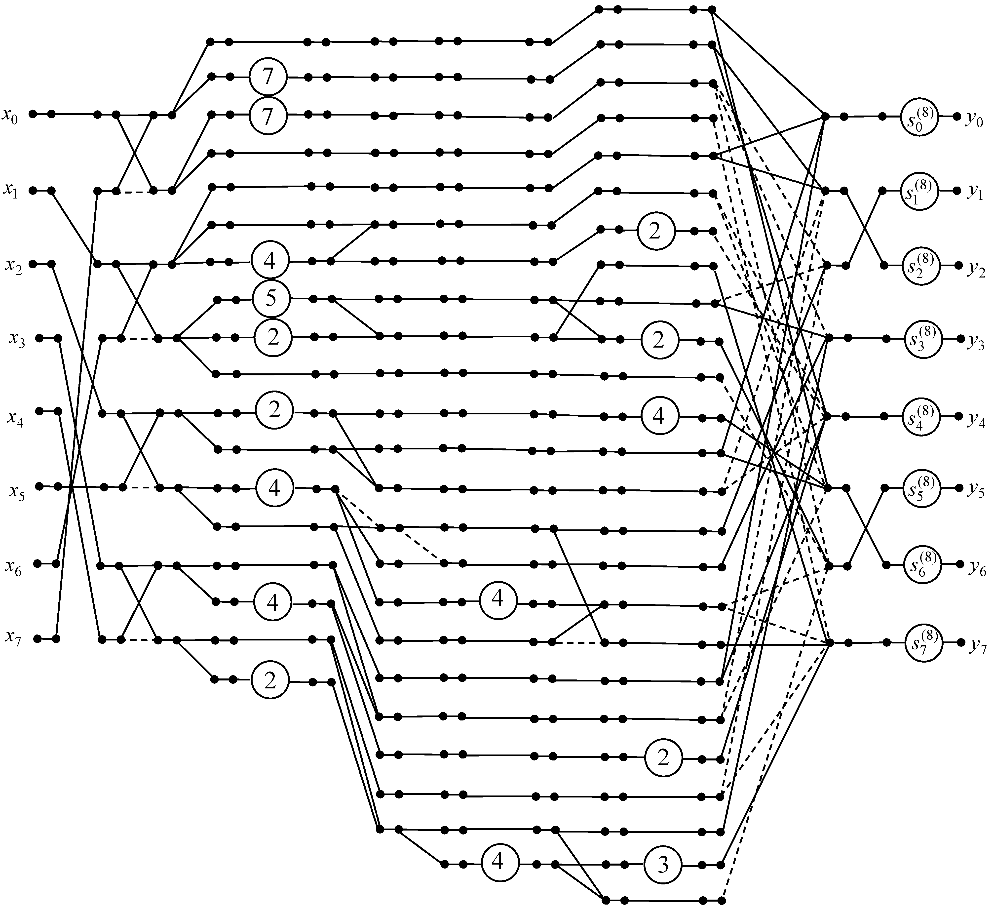
The repeated elements are contained in matrix ${\mathbf{C}}_8^{(b)}$. They facilitate the design of butterfly modules in the data flow graph for the 8-point 1D DTT calculation. An obtained data flow graph of the developed 8-point 1D DTT algorithm is presented in Figure 6.

Let us derive the factorization of the matrix of 8-point 1D DTT. We consider the matrices for computations on each layer of the graph. The matrices

$${\mathbf{W}}_8={\mathbf{H}}_2\oplus {\mathbf{H}}_2\oplus {\mathbf{H}}_2\oplus {\mathbf{H}}_2\mathrm{and}{\mathbf{W}}_{\mathbf{1}8\times 8}={\mathbf{1}}_{2\times 1}\oplus {\mathbf{1}}_{2\times 1}\oplus {\mathbf{1}}_{3\times 1}\oplus {\mathbf{1}}_{3\times 1}\oplus {\mathbf{1}}_{2\times 1}\oplus {\mathbf{1}}_{2\times 1}\oplus {\mathbf{1}}_{2\times 1}\oplus {\mathbf{1}}_{2\times 1}$$

(51)

are obtained at the first and second layers of the graph, respectively.

We have the diagonal matrix

$${\mathbf{D}}_{18}=\mathit{diag}(1,7,7,1,1,1,4,5,2,1,2,1,4,1,1,4,1,2)$$

(52)

at the third layer of calculation. The fourth, fifth and sixth layers of computations of the data flow graph in Figure 6 are implemented with the matrices ${\mathbf{W}}_{22\times 18}$, ${\mathbf{W}}_{23\times 22}$, and ${\mathbf{D}}_{23}$:

$${\mathbf{W}}_{22\times 18}={\mathbf{I}}_5\left[\begin{array}{cc}1& 1\\ & 1\end{array}\right]\oplus \left[\begin{array}{cc}1& \\ 1& 1\end{array}\right]\oplus 1\oplus \left[\begin{array}{cc}1& \\ & 1\\ 1& 1\end{array}\right]\oplus \left[\begin{array}{cc}-1& 1\\ 1& \\ 1& \\ & 1\end{array}\right]\oplus \left[\begin{array}{cc}1& \\ 1& 1\\ & 1\end{array}\right]\oplus \left[\begin{array}{cc}1& \\ 1& 1\end{array}\right],$$

(53)

$${\mathbf{W}}_{23\times 22}={\mathbf{I}}_{13}\oplus \left[\begin{array}{cc}1& \\ -1& 1\end{array}\right]\oplus {\mathbf{I}}_6\oplus \left[\begin{array}{c}1\\ 1\end{array}\right],$$

(54)

$${\mathbf{D}}_{23}=\mathit{diag}(1,1,1,1,1,1,1,1,1,1,1,1,1,1,1,4,1,1,1,1,1,1,4).$$

(55)

Let us define matrices ${\mathbf{T}}_{3\times 2}^{(1)}=\left[\begin{array}{cc}& 1\\ 1& \\ 1& 1\end{array}\right]$ and ${\mathbf{T}}_4=\left[\begin{array}{cccc}1& & & \\ & 1& & \\ & & 1& 1\\ 1& & & -1\end{array}\right]$.

Then, we obtain matrix ${\mathbf{W}}_{25\times 23}={\mathbf{I}}_7\oplus {\mathbf{T}}_{3\times 2}^{(1)}\oplus {\mathbf{I}}_4\oplus {\mathbf{T}}_4\oplus {\mathbf{I}}_4\oplus {\mathbf{T}}_{3\times 2}^{(3)}$, which provides calculations at the seventh layer of the data flow graph in Figure 6. Matrix ${\mathbf{T}}_{3\times 2}^{(3)}$ is defined by Equation (9). The computations at the eighth and ninth layers of the data flow graph in Figure 6 are provided with diagonal matrix ${\mathbf{D}}_{25}$ and matrix ${\mathbf{W}}_{8\times 25}$:

$${\mathbf{D}}_{25}=\mathit{diag}(1,1,1,1,1,1,2,1,1,2,1,4,1,1,1,1,1,1,1,1,2,1,1,3,1),$$

(56)

$${\mathbf{W}}_{8\times 25}==\left[\begin{array}{ccccccccccccccccccccccccc}1& & & & 1& & & & & & & & 1& & & & & & 1& & & & & & \\ & 1& & & 1& & & & & & & & & -1& & & & & & -1& & & & & \\ & & -1& & & & & & -1& & & & & & 1& & & & & & & -1& & & \\ & & -1& & & & & & 1& & & & & & & 1& & & & & & & 1& & \\ & 1& & & & -1& -1& & & & & & & -1& & & & & 1& & 1& & & & \\ 1& & & & & -1& & & & & & 1& 1& & & & & & & -1& & & & & \\ & & -1& & & & & & & 1& -1& & & & & & -1& & & & & & & & -1\\ & & & -1& & & & 1& & & & & & & & & -1& 1& & & & -1& & 1& \end{array}\right].$$

(57)

We multiply matrices ${\mathbf{P}}_8^{(1)}$, ${\mathbf{P}}_8^{(0)}$, ${\mathbf{W}}_{8\times 25}$, ${\mathbf{D}}_{25}$, ${\mathbf{W}}_{25\times 23}$, ${\mathbf{D}}_{23}$, ${\mathbf{W}}_{23\times 22}$, ${\mathbf{W}}_{22\times 18}$, ${\mathbf{D}}_{18}$, ${\mathbf{W}}_{18\times 8}$, and ${\mathbf{W}}_8$ with each other. As a result, the factorization of the 8-point 1D DTT matrix is obtained:

$${\mathbf{Y}}_{8\times 1}=\mathit{diag}({\mathbf{s}}_{8\times 1}){\mathbf{P}}_8^{(1)}{\mathbf{W}}_{8\times 25}{\mathbf{D}}_{25}{\mathbf{W}}_{25\times 23}{\mathbf{D}}_{23}{\mathbf{W}}_{23\times 22}{\mathbf{W}}_{22\times 18}{\mathbf{D}}_{18}{\mathbf{W}}_{18\times 8}{\mathbf{W}}_8{\mathbf{P}}_8^{(0)}{\mathbf{X}}_{8\times 1}.$$

(58)

We have presented some elements of diagonal matrices ${\mathbf{D}}_{18}$ and ${\mathbf{D}}_{25}$ as 7 = 8 − 1, 5 = 4 + 1, 3 = 2 + 1. It should be noted that initial 8-point real DTT requires 64 real-valued multiplications and 56 additions. Applying the proposed 8-point 1D DTT algorithm, we can reduce the number of real-valued multiplications to 8. Therefore, the total number of operations for the proposed 8-point 1D DTT algorithm is 53 additions, 8 real-valued multiplications, and 27 shifts.

3.7. Generalization of the Proposed Algorithms

Let us describe a generalization for N > 8 regarding the proposed N-point DTT algorithms, where N ranges from 3 to 8. The N-point DTT with N > 8 is also expressed by Equation (4). Further, we consider the even and odd lengths of input sequences separately.

At first, we suppose that N is even. Based on the symmetry of integer DTT, the following permutation of columns of the integer 1D DTT matrix ${\mathbf{C}}_N$ can be used:

$${\pi }_N=\left(\begin{array}{ccccccccc}1& 2& 3& 4& 5& 6& \text{…}& N-1& N\\ 1& N& 2& N-1& 3& N-2& \text{…}& N/2& N/2+1\end{array}\right).$$

(59)

Rearranging the rows is not necessary at all; however, if it is feasible to organize the rows such that pairs of equal-signed elements create 2 × 2 blocks, which can help minimize the number of additions and shifts required. This trick offers a reducing the number of integer multiplications.

Next, we start designing the data flow graph from inputs to outputs by adding the permutation of inputs at the first computational level. Then, we pairwise combine the outputs from the first computational level into butterfly modules and the outputs of each such module are transmitted to a line of integer multipliers. Every multiplication by an integer can be implemented by additions and shifts. The results of the multiplications are added together to obtain the outputs of integer DTT, and permutation of outputs is performed. The outputs of real DTT are calculated using the outputs of integer DTT multiplied by the specific coefficients as described in Equation (4).

Let us consider an odd N. The order of the columns of the integer DTT matrix ${\mathbf{C}}_N$ is changed using the permutation

$${\pi }_N=\left(\begin{array}{ccccccccc}1& 2& 3& 4& \text{…}& \left[N/2\right]& \left[N/2\right]+1& \left[N/2\right]+2& \text{…}\\ 1& N& 2& N-1& \text{…}& \left[N/2\right]& \left[N/2\right]+1& \left[N/2\right]+2& \text{…}\end{array}\right),$$

(60)

where $\left[N/2\right]$ denotes the whole part of $N/2$. Columns $\left[N/2\right]$, $\left[N/2\right]+1$, and $\left[N/2\right]+2$ remain in their places, and the remaining columns are grouped in pairs as in Equation (60). The symmetry of DTT is taken into account again.

The first and [N/2] + 1 rows are swapped. The order of the remaining rows can be left unchanged, or they can be swapped to reduce the number of multiplications and shifts as in the case of even N.

Next, we represent the transform matrix ${\mathbf{C}}_N^{(a)}$ after permutations as the sum of two matrices ${\mathbf{C}}_N^{(b)}$ and ${\mathbf{C}}_N^{(c)}$ of the same size as matrix ${\mathbf{C}}_N^{(a)}$:

$${\mathbf{C}}_N^{(a)}={\mathbf{C}}_N^{(b)}+{\mathbf{C}}_N^{(c)}$$

(61)

.

Matrix ${\mathbf{C}}_N^{(b)}$ includes the [N/2] + 1 row and the [N/2] + 1 column of matrix ${\mathbf{C}}_N^{(a)}$, and the rest of its elements are zero. In matrix ${\mathbf{C}}_N^{(c)}$, the [N/2] + 1 row and the [N/2] + 1 column are filled with zeros, and the rest of the elements are the same as in matrix ${\mathbf{C}}_N^{(a)}$. Then, matrix ${\mathbf{C}}_N^{(b)}$ has identical entries in its [N/2] + 1 row. This allows us to reduce the number of operations without further transformations. Next, we eliminate the row and column containing only zero entries in matrix ${\mathbf{C}}_N^{(c)}$ and obtain matrix ${\mathbf{C}}_{N-1}^{(c)}$. Matrix ${\mathbf{C}}_{N-1}^{(c)}$ has an even size. Therefore, a data flow graph of the fast algorithm for the transform with matrix ${\mathbf{C}}_{N-1}^{(c)}$ can be constructed similarly to the previous case.

To obtain the data flow graph for the transform with matrix ${\mathbf{C}}_N^{(a)}$, we add the path, corresponding to the [N/2] + 1 output after the column permutation, to the data flow graph for the transform with matrix ${\mathbf{C}}_{N-1}^{(c)}$. The edges of the resulting graph that enter the node at this path immediately after column permutation are constructed using a structural approach similar to the case of N = 7. Again, for odd N, the outputs of integer DTT after row permutation are multiplied by the specific coefficients to obtain the outputs of real DTT.

4. Results

We used the MATLAB R2023b software for the experimental research of the proposed algorithms. The correctness of the designed algorithms was tested. For this, the DTT matrices were obtained using Equations (4)–(6) for N = 3, 4, 5, 6, 7, 8 at first. Next, the factorizations of 1D DTT matrices were calculated with the expressions (7), (10), (20), (32), (46), and (58). The correctness of the proposed algorithms was indicated via the coincidence of the elements of 1D DTT matrices and the elements of the products of the matrices included in the factorizations of the DTT matrices for the same N.

Further, the computational complexity of the developed algorithms was evaluated, and the results are illustrated in

Table 1. The number of multiplications, additions, and shifts performed by the proposed algorithms and the direct matrix-vector products.

N	Direct Method		Proposed Algorithms
	Adds.	Mults.	Adds.	Mults.	Shifts
3	5	8	5 (0%)	3 (−62%)	1
4	12	8	9 (−25%)	2 (−75%)	5
5	18	23	19 (+5%)	5 (−78%)	6
6	30	36	27 (−10%)	6 (−83%)	15
7	37	44	37 (0%)	7 (−84%)	22
8	56	64	53 (−5%)	8 (−87%)	27

. In parentheses, we show the difference in the number of operations as a percentage. The minus sign indicates a reduction in the number of operations compared to the direct method, while the plus sign indicates an increase. As can be seen from Table 1, the number of multiplications decreased by an average of 78% for N = 3, 4, 5, 6, 7, 8. At the same time, the number of additions decreased by an average of 5% for the same N. The calculation of the direct matrix-vector product for N = 4 additionally requires 8 shifts.

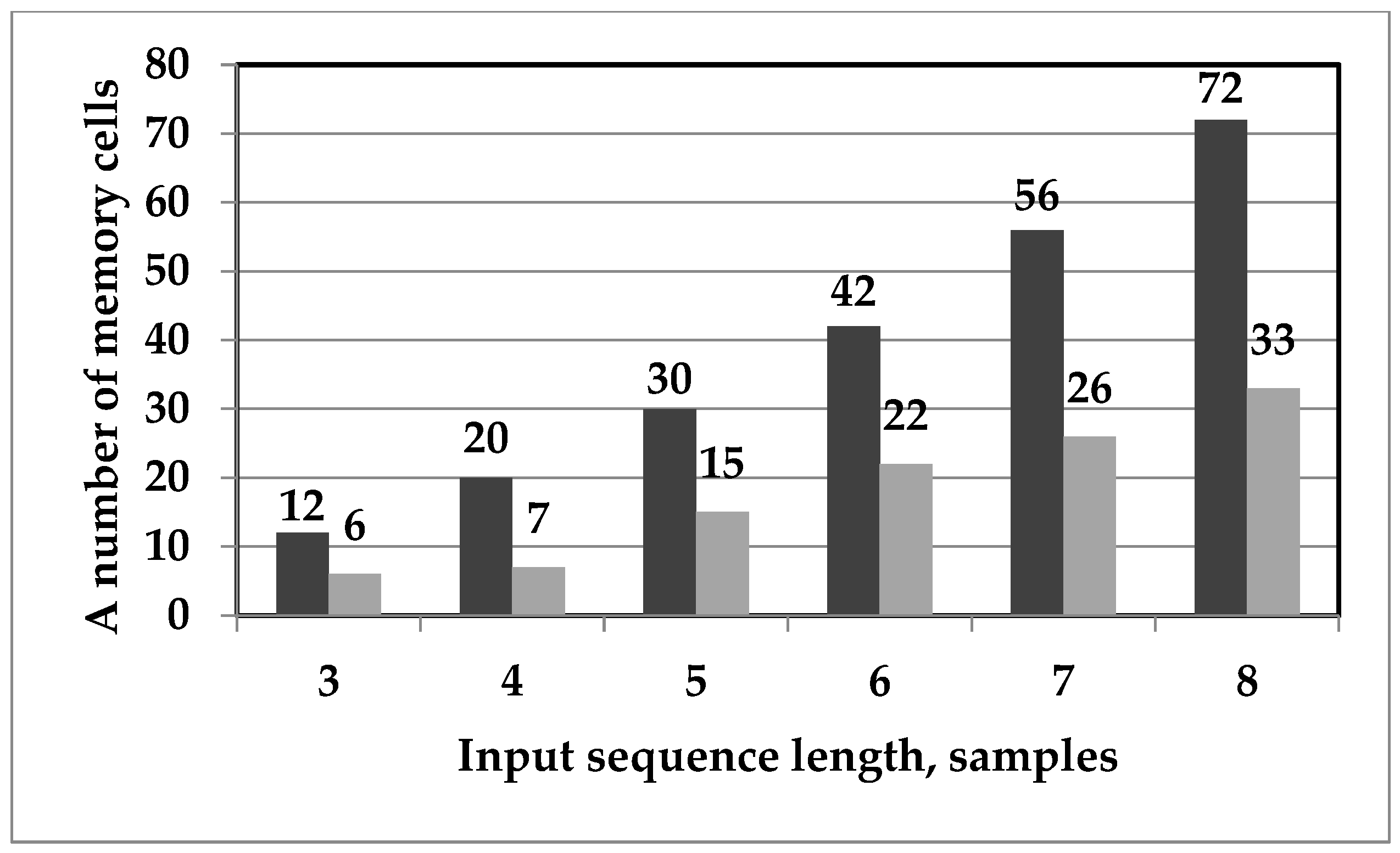
After evaluating the effectiveness of the solutions by calculating the number of arithmetic operations required to implement the obtained algorithms, the additional evaluations’ memory consumption is provided in Figure 7. The proposed real DTT algorithms required 54% less memory than the direct matrix-vector product.

The evaluation of memory costs for the proposed algorithms demonstrates their limitations. However, unlike the evaluation of arithmetic complexity, the memory costs depend on the method of implementing the algorithm and the platform on which the algorithm is implemented. In addition, memory consumption is also affected by the skill and experience of the designer. In general, the proposed algorithms allow both software and hardware implementation. Moreover, both software and hardware implementation can use various approaches and tricks, that lead to certain memory costs, time delays, and hardware resource usage. As for memory, the calculations can be implemented so that the same memory cells are used at each subsequent stage of algorithm implementation if such a possibility exists. The proposed algorithms can be implemented sequentially, in parallel, or in parallel sequentially, depending on the structure and capabilities of the implementation platform. This implementation affects the time delay in obtaining results.

A deeper analysis shows that when implementing the proposed algorithms at the hardware level using maximum parallelization of calculations, intermediate memory in asynchronous mode may not be needed. If we organize pipeline processing, then we have to insert time delays that align the data flow. In this case, additional buffer memory will be needed. Thus, the evaluation of the efficiency of algorithmic solutions in terms of memory requirements, although it somehow characterizes these solutions, is very subjective. Therefore, since we do not consider implementation issues, it is the evaluation of arithmetic complexity that is, although not exhaustive, the most reliable and accurate characteristic of the efficiency of the proposed solutions.

5. Discussion of Computational Complexity

In

Table 2. The number of operations for the existing algorithms.

Algorithm	Reference, Year of Publication	$\mathit{N}=\mathbf{4}$			$\mathit{N}=\mathbf{8}$
		Mults.	Adds.	Shifts	Mults.	Adds.	Shifts
Gogoi, Peesapati	[8], 2019	6 (−67%)	8 (+12%)	2 (+150%)	29 (−72%)	32 (+66%)	12 (+125%)
Prattipati, Ishwar, Swamy, Meher	[1], 2013	–	–	–	8 (0%)	44 (+20%)	29 (−7%)
Ishwar, Meher, Swamy	[41], 2008	2 (0%)	10 (−10%)	4 (+25%)	–	–	–
Proposed algorithm	–	2	9	5	8	53	27

, we present the number of additions, shifts, and multiplications for the 1D DTT algorithms known from the literature. It is important to note that in references [1,41], the number of additions and shifts for integer DTT was evaluated. Therefore, we added to the corresponding rows of Table 2 the minimal number of multiplications needed to implement real DTT. As a consequence, the results in Table 2 show that the number of multiplications for the proposed algorithm is the same for N = 4 and N = 8 as compared with [1,41]. At the same time, we reduced the multiplication by 67–72% compared with [8]. However, the number of additions increased by 12–66%, and additional shifts are required.

The advantage of the proposed solutions is that the length of the input data sequence for the proposed DTT fast algorithms is not limited by 4 and 8. The obtained algorithms are multiplier-free for integer DTT. They can calculate integer DTT and real DTT. The data flow graphs constructed for the proposed algorithms have a modular structure that is well-suited for hardware implementation. A carefully selected heuristic for certain values of N can greatly decrease the computational complexity of the DTT algorithm, as in [1]. However, extending the proposed algorithms to cases where N is greater than 8 enables the design of a fast DTT algorithm for input sequences of any length.

6. Conclusions

In this paper, the algorithms for real DTT with reduced multiplicative complexity are developed by combining sparse matrix factorization with the structural approach. The obtained algorithms have butterfly architecture and are multiplication-free for the integer DTT. The combination of the structural approach with sparse matrix factorization enables the design of fast algorithms without restricting input sequence length to 4 or 8. A matrix factorization of each proposed solution was constructed with sparse diagonal and quasi-diagonal matrices. Another advantage of the obtained algorithms is that their representation via the data flow graphs provides a layout for the VLSI implementation of the proposed solutions.

The computational complexity of the proposed algorithms was compared with the computational complexity of direct matrix-vector products. As a result, it was found that the obtained factorizations of real DTT matrices reduce the number of multiplications by an average of 78% in the range of signal lengths from 3 to 8. Meanwhile, the average number of additions in the same range of signal lengths decreased by nearly 5%. Although additional shifts are required instead of multiplications, they are less time- and resource-consuming.

Comparison with fast DTT algorithms known from the literature was provided for input signal lengths 4 and 8. It was shown that the proposed algorithms have the same or slightly worse computational complexity. The latter is caused by the versatility of combining the structural approach with a sparse matrix factorization compared to the specificity of existing solutions.

Future research development may involve constructing a fast orthogonal projection of DTT using the Kronecker product. Reducing the computational complexity of this form of DTT may be used in applications such as speech enhancement [42] and filter design [43].